Improved State-Space Approach Based on Lumped Mass Matrix for Transient Analysis of Large-Scale Locally Nonlinear Structures

Abstract

Due to the assumption of acceleration variation in traditional step-by-step integration methods such as Newmark, sufficiently small time steps are required to ensure numerical stability and accuracy in dynamic systems. In contrast, the state-space approach, based on piecewise interpolation of discrete load functions, does not rely on predetermined acceleration assumptions and has demonstrated high efficiency in terms of stability and accuracy. The original state-space method requires the calculation of the inverse of the structural mass in the transition matrix. However, when a lumped mass matrix is used, this computation renders the entire mass matrix singular, resulting in an invalid solution expression. To address this issue, this study proposes an improved state-space approach for the transient analysis of large-scale structural systems with local nonlinearities. In this approach, a nonlinear force corrector is introduced as an external force term applied to the linear elastic system to account for the nonlinear behavior of locally yielding components. Consequently, the original nonlinear dynamic system can be transformed into an equivalent linear elastic transient system. Furthermore, based on the lumped mass matrix, a first-order ordinary differential state-space equation for such an equivalent linear elastic transient system is derived. Simulation results from three transient system examples show that the state-space approach outperforms the Newmark method in terms of accuracy and stability for dynamic systems characterized by high frequency and low damping. The prediction results show that the state-space approach appears to be insignificantly affected by the choice of the consistent or lumped mass matrix. The numerical results show that the root-mean-square errors between the consistent and lumped matrices in the top displacement time histories of a 15-storey plane frame under various seismic intensities are all less than 1%, and in the base reaction time histories responses the discrepancies are only about 0.5%, indicating that the use of lumped mass matrices is quite reliable. When many nodes or degrees of freedom have no assigned mass, the dimensionality of the state-space equation can be significantly reduced using the lumped mass approach. Therefore, the simulation of large-scale systems can be simplified by employing the improved state-space approach with lumped mass matrices, yielding results nearly identical to those obtained using traditional methods. In conclusion, the improved state-space approach has great potential for the simulation of transient behavior in large-scale systems with local nonlinearities.

1. Introduction

The dynamic characteristics of structures under seismic loads are crucial for the analysis, design, and safety assessment of engineering structures. Numerical, experimental, and hybrid simulations are commonly employed methods to obtain these dynamic responses. However, due to limitations in laboratory conditions, time, and economic costs, experimental and hybrid simulations are less popular compared to numerical methods. Among numerical approaches, step-by-step integration methods are widely used for analyzing transient systems, whether linear or nonlinear. These step-by-step integration methods include both explicit algorithms (e.g., central difference [1]) and implicit algorithms (e.g., Newmark-β [2], Wilson-θ [3]).

The implicit step-by-step integration method is the most widely used; however, the computational effort required for simulating large-scale time-varying nonlinear structural systems is substantial. These approaches necessitate calculating the high-dimensional structural stiffness matrix and determining the state of numerous discrete elements at each time step [3,4,5]. To enhance efficiency, three distinct efforts have been made in the conventional implicit step-by-step integration method: (1) reducing the matrix order of the structural stiffness [6]; (2) minimizing the number of matrix operations (e.g., formation and decomposition [7]) involved in handling the large-scale structural stiffness; and (3) streamlining the operations for element state determinations [8]. As discussed in the literature [8], a nonlinear force corrector (NFC) is proposed and considered as the external force applied to the structure. This allows the original nonlinear system to be transformed into a linear one, where the nonlinear behavior of yielding components or elements is accounted for through the application of the structural NFC on the linear system. Since the equivalent system is linear and elastic, the global stiffness matrix only needs to be formed and decomposed once. Furthermore, the structural NFC is solely influenced by those yielding components or elements. Consequently, when the large-scale structure exhibits local material nonlinearities, i.e., the ratio of yielding to total elements is very small, the computational effort required for element state determinations is, therefore, not significant.

All numerical procedures in these step-by-step integration methods rely on the assumption of variation in structural acceleration over discrete time intervals [9,10]. For instance, the Newmark method assumes either constant or linear acceleration variation. Consequently, these methods are highly dependent on the chosen time step size, which should typically be sufficiently small to ensure stability and accuracy of the dynamic system [11,12]. The state-space approach (SSA), which is considered an alternative to the aforementioned conventional methods, exhibits significant potential in simulating the dynamic behavior of both linear and nonlinear structural systems [9,13,14,15,16,17,18,19,20,21,22]. The SSA demonstrates notable effectiveness in terms of numerical stability and accuracy. In contrast to the step-by-step integration method, the SSA utilizes piecewise interpolation of discrete load functions, enabling convolutional integration [15]. Due to the absence of forced acceleration assumptions in the SSA, the distortion of the system’s dynamic characteristics is relatively mild compared to the step-by-step method. Through a frequency domain analysis of a linear single degree of freedom (SDOF) system, as presented in Appendix A of the referenced literature [15], the simulation results obtained using the SSA closely align with the analytical solutions, while the Newmark method exhibits some sensitivity to the time step used.

In the analytical solution of the SSA, the exponential power of the transition matrix can be computed using Pade approximation [23], Taylor series expansion [24], or precise integration methods [25]. Regardless of the method chosen, calculating the inverse of the structural mass is required for the transition matrix. When employing the consistent mass (CM) matrix, the assembled structural mass will be a full-rank non-diagonal matrix [11]. However, if the lumped mass (LM) matrix is used, it becomes a diagonal matrix and may become singular if mass is not assigned to certain nodes or degrees of freedom (DOFs). In such cases, the inverse of the mass matrix cannot be computed, rendering the original state-space solution expression unsuitable for computing the dynamic response of the system.

To address the aforementioned limitation, this study introduces an improved SSA that utilizes the LM matrix for conducting transient simulations of large-scale structures with local nonlinearities. This approach incorporates the concept of the NFC mentioned above and reformulates the recursive formula of the SSA. For simplicity, two-dimensional (2D) Euler–Bernoulli beam (EBB) frames are employed as the research subjects. The subsequent sections of this study are organized as follows: Section 2 provides an overview of the fundamental theories, including the uniaxial stress–strain constitutive model, the section stress–deformation relationship, the element force–displacement relationship of the EBB element, the equation of the linear viscous damper, the CM and LM matrices of the EBB element, the structural governing equation, and the original SSA formulation. Section 3 presents the derivation of the improved SSA method. Section 4 details the numerical implementation of the enhanced SSA. Finally, Section 5 demonstrates the application of the method through example scenarios.

2. Basic Theory

2.1. Uniaxial Stress–Strain Relationship

In plastic theory [26], the actual stress $\sigma$ of a uniaxial material can be divided into an elastic trial stress ${\sigma }_t$ and a plastic stress corrector ${\sigma }_p$ [8], yielding the following:

$$\sigma ={\sigma }_t+{\sigma }_p=E\cdot ϵ+{\sigma }_p,$$

(1)

where $E$ is the elastic modulus and $ϵ$ is the strain of the uniaxial material. Note that the plastic stress corrector ${\sigma }_p$ accounts for the nonlinearity due to yielding within the material, which vanishes when there is no yielding.

2.2. Sectional Force–Deformation Relationship of EBB Element

The sectional force–deformation relationship of an Euler–Bernoulli beam (EBB) element in the basic coordinate system is defined by the interaction between the sectional stress resultant $\mathit{s}$ and the sectional deformation $\mathit{e}$. The relationship is given by the following:

$$\mathit{s}={\mathit{d}}_s\mathit{e}+{\mathit{s}}_p,$$

(2)

where ${\mathit{d}}_s$ is the initial sectional stiffness matrix, expressed as follows:

$${\mathit{d}}_s={\int }_A{\mathit{l}}^{T}E\mathit{l}dA.$$

Here, $\mathit{l}=\left[\begin{array}{cc}1& -y\end{array}\right]$, and y is the y-coordinate of the material point in the section. The sectional deformation $\mathit{e}$ of the beam can be written as follows:

$$\mathit{e}=\mathit{b}{\mathit{v}}_e,$$

(3)

where $\mathit{b}={\displaystyle \frac{1}{L}}\left[\begin{array}{ccc}1& 0& 0\\ 0& {\displaystyle \frac{6x}{L}}-4& {\displaystyle \frac{6x}{L}}-2\end{array}\right]$ is the linear strain–displacement matrix [11], L is length of the beam element, and ${\mathit{v}}_e$ is the nodal displacement in the basic coordinate system.

In Equation (2), ${\mathit{s}}_p$ is the plastic stress resultant corrector of the section defined as follows:

$${\mathit{s}}_p={\int }_A{\mathit{l}}^T{\sigma }_{p}dA.$$

(4)

2.3. Force–Displacement Relationship of EBB Element

According to the principle of virtual work, the resisting force ${\mathit{q}}_e$ of the EBB element in the basic coordinate system can be calculated by integrating the sectional stress resultant $\mathit{s}$ along the length of the beam as follows:

$${\mathit{q}}_e={\int }_0^L{\mathit{b}}^T\mathit{s}dx$$

(5)

Substituting Equations (2) and (3) into Equation (5) results in the following:

$${\mathit{q}}_e={\mathit{D}}_e{\mathit{v}}_e+{\mathit{q}}_e^c,$$

(6)

where ${\mathit{D}}_e$ and ${\mathit{q}}_e^c$ are the initial stiffness and nonlinear force corrector (NFC) of the beam element in the basic coordinate system, respectively, yielding the following:

$${\mathit{D}}_e={\int }_0^L{\mathit{b}}^T{\mathit{d}}_s\mathit{b}dx \mathrm{and} {\mathit{q}}_e^c={\int }_0^L{\mathit{b}}^T{\mathit{s}}_{p}dx.$$

(7)

Transforming the basic coordinate system into a global one using the relationship ${\mathit{v}}_e={\mathit{T}}_e{\mathit{u}}_e$ (where ${\mathit{T}}_e$ is the transformation matrix relating the global and basic coordinate systems and ${\mathit{u}}_e$ is the global displacement vector of the beam element), Equation (6) can be re-expressed as follows [8]:

$${\mathit{r}}_e={\mathit{k}}_e{\mathit{u}}_e+{\mathit{f}}_e^c,$$

(8)

where ${\mathit{r}}_e={\mathit{T}}_e^T{\mathit{q}}_e$, ${\mathit{k}}_e={\mathit{T}}_e^T{\mathit{D}}_e{\mathit{T}}_e$, and ${\mathit{f}}_e^c={\mathit{T}}_e^T{\mathit{q}}_e^c$ are the resisting force, initial stiffness matrix, and NFC of the element in the global coordinate system, respectively.

2.4. Equation of Motion of EBB Element

More generally, the equation of motion of the beam element under the seismic loading can be written as follows [27]:

$${\mathit{m}}_e{\ddot{\mathit{u}}}_e\left(t\right)+{\mathit{c}}_e{\dot{\mathit{u}}}_e\left(t\right)+{\mathit{r}}_e=-{\mathit{m}}_e{\mathit{i}}_e{\ddot{u}}_g\left(t\right),$$

(9)

where ${\mathit{m}}_e$ and ${\mathit{c}}_e$ are the mass and damping matrices of the element, respectively; the superscripts single dot and double dot indicate the first and second derivatives of a variable with respect to time t, respectively; ${\mathit{i}}_e$ is the influence vector of the element; ${\ddot{u}}_g$ is the scalar ground acceleration.

Based on the consistent element mass matrix [11], the mass matrix of the 2D EBB element can be expressed as the following:

$${\mathit{m}}_e={\displaystyle \frac{\rho AL}{420}}\left[\begin{array}{cccccc}140& 0& 0& 70& 0& 0\\ 0& 156& 22L& 0& 54& -13L\\ 0& 22L& 4L^2& 0& 13L& -3L^2\\ 70& 0& 0& 140& 0& 0\\ 0& 54& 13L& 0& 156& -22L\\ 0& -13L& -3L^2& 0& -22L& 4L^2\end{array}\right],$$

where $\rho$ is the density of the beam, $L$ is the length of the beam, and $A$ is the area of the beam element section. While using the lumped element mass matrix, it can be written as the following:

$${\mathit{m}}_e={\displaystyle \frac{\rho AL}{2}}\left[\begin{array}{cccccc}1& 0& 0& 0& 0& 0\\ 0& 1& 0& 0& 0& 0\\ 0& 0& 0& 0& 0& 0\\ 0& 0& 0& 1& 0& 0\\ 0& 0& 0& 0& 1& 0\\ 0& 0& 0& 0& 0& 0\end{array}\right].$$

2.5. Equation of Linear Viscous Damper

The damping force $f^{\mathrm{vd}}$ of a viscous damper can be expressed as follows [28]:

$$f_d=c{\dot{u}}^{\alpha }$$

(10)

where c is the damping coefficient, $\alpha$ is the velocity index, and $\dot{u}$ is the velocity of the damper. In a structure equipped with viscous dampers, the damping force of the kth damper connecting nodes i and j can be computed as follows:

$$f_d^k=c{\mathit{T}}_k{\left({\dot{\mathit{u}}}_i-{\dot{\mathit{u}}}_j\right)}^{\alpha }$$

(11)

where ${\mathit{T}}_k=\left[\begin{array}{cc}\mathit{cos}{\theta }_k& \mathit{cos}{\phi }_k\end{array}\right]$ is the transformation matrix in 2D models (${\theta }_k$ and ${\phi }_k$ are the angles of the viscous damper with respected to the x-axis and y-axis, respectively). In this study, for simplicity, the linear viscous damper (LVD) is used, where $\alpha$ is taken as 1.

Then, the resisting force ${\mathit{r}}_d^k$ of the kth LVD can be written as follows:

$${\mathit{r}}_d^k={\mathit{C}}_d^k\dot{\mathit{u}}$$

(12)

where

$${\mathit{r}}_d^k=\left\{\begin{array}{c}\mathbf{0}\\ ⋮\\ {\mathit{r}}_{d,i}^k\\ ⋮\\ {\mathit{r}}_{d,j}^k\\ ⋮\\ \mathbf{0}\end{array}\right\}, \dot{\mathit{u}}=\left\{\begin{array}{c}{\dot{\mathit{u}}}_1\\ ⋮\\ {\dot{\mathit{u}}}_i\\ ⋮\\ {\dot{\mathit{u}}}_j\\ ⋮\\ {\dot{\mathit{u}}}_n\end{array}\right\}, {\mathit{C}}_d^k=\left[\begin{array}{ccccccc}\mathbf{0}& & & & & & \\ & \ddots & & & & & \\ & & {\mathit{E}}_k& & -{\mathit{E}}_k& & \\ & & & \ddots & & & \\ & & -{\mathit{E}}_k& & {\mathit{E}}_k& & \\ & & & & & \ddots & \\ & & & & & & \mathbf{0}\end{array}\right], {\mathit{E}}_k=c_k{\mathit{T}}_k{\mathit{T}}_k^T.$$

Subsequently, the assembled resisting force of all LVDs can be obtained as the following:

$${\mathit{r}}_d={\mathit{C}}_d\dot{\mathit{u}}$$

(13)

where ${\mathit{C}}_d={\sum }_{k=1}^p{\mathit{C}}_d^k$ is the damping matrix of the LVDs, and p is the number of LVDs.

2.6. Structural Governing Equation

After substitution of Equation (8) into Equation (9), the equation of motion of a n-dimensional structural system equipped with LVDs can be assembled as the following:

$$\mathit{M}\ddot{\mathit{u}}+\left(\mathit{C}+{\mathit{C}}_d\right)\dot{\mathit{u}}+\mathit{K}\mathit{u}=-\mathit{M}\mathit{i}{\ddot{u}}_g-{\mathit{f}}^c,$$

(14)

where $\mathit{M}={\sum }_{N_E}{\mathit{m}}_e$, $\mathit{K}={\sum }_{N_E}{\mathit{k}}_e$, and $\mathit{C}={\sum }_{N_E}{\mathit{c}}_e$ are the n × n mass, initial stiffness, and damping matrices of the structure, respectively; $\mathit{u}={\sum }_{N_E}{\mathit{u}}_e$ is the $n\times 1$ displacement vector of the structure; $\mathit{i}={\sum }_{N_E}{\mathit{i}}_e$ is an n × 1 influence vector of the structure; ${\mathit{f}}^c={\sum }_{N_E}{\mathit{f}}_e^c$ is the NFC of the structure; $N_E$ is the number of discrete elements. Note that the NFC ${\mathit{f}}^c$ is only contributed by nonlinear elements, i.e., ${\mathit{f}}^c={\sum }_{N_{\mathrm{YE}}}{\mathit{f}}_e^c$ ($N_{\mathrm{YE}}$ is the number of yielding elements). In this study, the Rayleigh damping model that is proportional to the mass and initial stiffness of the structure is utilized, i.e., $\mathit{C}=a_0\mathit{M}+a_1\mathit{K}$, where $a_0$ and $a_1$ are the coefficients corresponding to the mass and initial stiffness matrices, respectively.

It is essential to highlight that the consistent element mass matrix, discussed previously, is a non-diagonal matrix with full rank. Conversely, the LM matrix is a diagonal matrix that does not have full rank. Therefore, utilizing the consistent element mass matrix results in the assembled structural mass matrix M being non-diagonal and full rank. Conversely, employing the LM matrix leads to the assembled structural mass matrix being diagonal but lacking full rank.

2.7. Original State-Space Approach (SSA)

Based on the CM matrix, the state variable of the structural system can be defined as $\mathit{z}\left(t\right)=\left\{\begin{array}{c}\mathit{u}\left(t\right)\\ \dot{\mathit{u}}\left(t\right)\end{array}\right\}$; then, Equation (14) can be transformed into the state-space form as follows [14]:

$$\dot{\mathit{z}}\left(t\right)=\mathit{A}\mathit{z}\left(t\right)+\mathit{h}\left(t\right)+\mathit{p}\left(t\right),$$

(15)

where $\mathit{A}=\left[\begin{array}{cc}\mathbf{0}& \mathit{I}\\ -{\mathit{M}}^{-1}\mathit{K}& -{\mathit{M}}^{-1}\left(\mathit{C}+{\mathit{C}}_d\right)\end{array}\right]$ is the $2n\times 2n$ transition matrix, $\mathit{h}=\left\{\begin{array}{c}\mathbf{0}\\ -\mathit{i}{\ddot{u}}_g\end{array}\right\}$ is a 2n × 1 control vector related to the external seismic excitation, and $\mathit{p}=\left\{\begin{array}{c}\mathbf{0}\\ {\mathit{M}}^{-1}{\mathit{f}}^c\end{array}\right\}$ is a 2n × 1 control vector relying on the structural NFC. Here, 0 is an n-order zero matrix in A and n-dimensional zero vector in h and p, and I is an n-order identity matrix.

If the state variable at the current time $t_i$ is known, the state variable at the next time step $t_{i+1}$ can be calculated using the following equation:

$$\mathit{z}\left(t_{i+1}\right)=e^{\mathit{A}\Delta t}\mathit{z}\left(t_i\right)+{\int }_0^{\Delta t}{e}^{\mathit{A}\left(\Delta t-\tau \right)}\mathit{h}\left(\tau +t_i\right)d\tau +{\int }_0^{\Delta t}{e}^{\mathit{A}\left(\Delta t-\tau \right)}\mathit{p}\left(\tau +t_i\right)d\tau ,$$

(16)

where $\Delta t=t_{i+1}-t_i$ is the time step. Generally, the ground acceleration ${\ddot{u}}_g$ is regarded as linearly varying within any time step; then, $\mathit{h}\left(t\right)={\displaystyle \frac{t_{i+1}-t}{\Delta t}}\mathit{h}\left(t_i\right)+{\displaystyle \frac{t-t_i}{\Delta t}}\mathit{h}\left(t_{i+1}\right)$. In this study, p is also assumed to be linearly varying in the time interval $\left[t_i,t_{i+1}\right]$, i.e., $\mathit{p}\left(t\right)={\displaystyle \frac{t_{i+1}-t}{\Delta t}}\mathit{p}\left(t_i\right)+{\displaystyle \frac{t-t_i}{\Delta t}}\mathit{p}\left(t_{i+1}\right)$; then,

$${\mathit{z}}_{i+1}={\mathit{\Phi }}_1{\mathit{z}}_i+{\mathit{\Phi }}_3{\mathit{h}}_i+{\mathit{\Phi }}_4{\mathit{h}}_{i+1}+{\mathit{\Phi }}_3{\mathit{p}}_i+{\mathit{\Phi }}_4{\mathit{p}}_{i+1},$$

(17)

where ${\mathit{\Phi }}_1=e^{\mathit{A}\Delta t}$, ${\mathit{\Phi }}_2={\displaystyle \frac{\left(e^{\mathit{A}\Delta t}-\mathit{I}\right){\mathit{A}}^{-1}}{\Delta t}}$, ${\mathit{\Phi }}_3={\mathit{\Phi }}_2\Delta t-{\mathit{\Phi }}_4$, ${\mathit{\Phi }}_4=\left({\mathit{\Phi }}_2-\mathit{I}\right){\mathit{A}}^{-1}$ ${\mathit{z}}_{i+1}=\mathit{z}\left(t_{i+1}\right)$, ${\mathit{z}}_i=\mathit{z}\left(t_i\right)$, ${\mathit{h}}_i=\mathit{h}\left(t_i\right)$, ${\mathit{h}}_{i+1}=\mathit{h}\left(t_{i+1}\right)$, ${\mathit{p}}_i=\mathit{p}\left(t_i\right)$, and ${\mathit{p}}_{i+1}=\mathit{p}\left(t_{i+1}\right)$.

3. Improved State-Space Approach (I-SSA)

However, when using the lumped element mass matrix, the structural mass matrix M may become singular if masses are not assigned at some nodes or DOFs in a discrete finite element (FE) model. Under this circumstance, the inverse matrix ${\mathit{M}}^{-1}$ in the transition matrix A cannot be obtained. To address this issue, an improved SSA will be introduced in this section. The equation of motion (14) can be rewritten in block form as follows:

$$\begin{gathered} \left[\begin{array}{cc}{\mathit{M}}_1& \\ & \mathbf{0}\end{array}\right]\left\{\begin{array}{c}{\ddot{\mathit{u}}}_1\\ {\ddot{\mathit{u}}}_2\end{array}\right\}+\left[\begin{array}{cc}{\mathit{C}}_{11}+{\mathit{C}}_{d,11}& {\mathit{C}}_{12}+{\mathit{C}}_{d,12}\\ {\mathit{C}}_{21}+{\mathit{C}}_{d,21}& {\mathit{C}}_{22}+{\mathit{C}}_{d,22}\end{array}\right]\left\{\begin{array}{c}{\dot{\mathit{u}}}_1\\ {\dot{\mathit{u}}}_2\end{array}\right\} \\ +\left[\begin{array}{cc}{\mathit{K}}_{11}& {\mathit{K}}_{12}\\ {\mathit{K}}_{21}& {\mathit{K}}_{22}\end{array}\right]\left\{\begin{array}{c}{\mathit{u}}_1\\ {\mathit{u}}_2\end{array}\right\}=-\left[\begin{array}{cc}{\mathit{M}}_1& \\ & \mathbf{0}\end{array}\right]\left\{\begin{array}{c}{\mathit{i}}_1\\ {\mathit{i}}_2\end{array}\right\}{\ddot{u}}_g+\left\{\begin{array}{c}{\mathit{f}}_1^c\\ {\mathit{f}}_2^c\end{array}\right\}, \end{gathered}$$

(18)

where ${\mathit{M}}_1$ is an m $\times$ m mass sub-matrix with full rank, and m is less than n.

For the Rayleigh damping matrix $\mathit{C}=a_0\mathit{M}+a_1\mathit{K}$, we have ${\mathit{C}}_{11}=a_0{\mathit{M}}_1+a_1{\mathit{K}}_{11}$, ${\mathit{C}}_{12}=a_1{\mathit{K}}_{12}$, ${\mathit{C}}_{21}=a_1{\mathit{K}}_{21}$, and ${\mathit{C}}_{22}=a_1{\mathit{K}}_{22}$. Subsequently, the second item of Equation (18) yields the following:

$$\left\{\begin{array}{c}{\mathit{u}}_2={\mathit{K}}_{22}^{-1}{\mathit{f}}_2^c-{\mathit{\Gamma }}_1{\mathit{u}}_1\\ {\dot{\mathit{u}}}_2=-\left({\mathit{\Gamma }}_1+{\mathit{\Gamma }}_2\right){\dot{\mathit{u}}}_1 \end{array}\right.,$$

(19)

where ${\mathit{\Gamma }}_1={\mathit{K}}_{22}^{-1}{\mathit{K}}_{21}$ and ${\mathit{\Gamma }}_2={\displaystyle \frac{1}{a_1}}{\mathit{K}}_{22}^{-1}{\mathit{C}}_{d,21}$.

Consequently, the reduced governing equation can be derived from the first item of Equation (18) as follows:

$${\mathit{M}}_1{\ddot{\mathit{u}}}_1+{\overline{\mathit{C}}}_{11}{\dot{\mathit{u}}}_1+{\overline{\mathit{K}}}_{11}{\mathit{u}}_1=-{\mathit{M}}_1{\mathit{i}}_1{\ddot{u}}_g+{\overline{\mathit{f}}}_1^c,$$

(20)

where ${\overline{\mathit{C}}}_{11}={\mathit{C}}_{11}+{\mathit{C}}_{12}\left({\mathit{\Gamma }}_1+{\mathit{\Gamma }}_2\right)+{\mathit{C}}_{d,11}-{\mathit{C}}_{d,12}\left({\mathit{\Gamma }}_1+{\mathit{\Gamma }}_2\right)$, ${\overline{\mathit{K}}}_{11}={\mathit{K}}_{11}-{\mathit{K}}_{12}{\mathit{K}}_{22}^{-1}{\mathit{K}}_{21}$, and ${\overline{\mathit{f}}}_1^c={\mathit{f}}_1^c-{\mathit{K}}_{12}{\mathit{K}}_{22}^{-1}{\mathit{f}}_2^c$. For the structural system without LVDs, ${\mathit{C}}_d=\mathbf{0}$ and ${\mathit{\Gamma }}_2=\mathbf{0}$, then ${\overline{\mathit{C}}}_{11}=a_0{\mathit{M}}_1+a_1{\overline{\mathit{K}}}_{11}$.

Let the state variable of the reduced system (20) be defined as $\overline{\mathit{z}}=\left\{\begin{array}{c}{\mathit{u}}_1\\ {\dot{\mathit{u}}}_1\end{array}\right\}$; then,

$$\dot{\overline{\mathit{z}}}=\overline{\mathit{A}}\overline{\mathit{z}}+\overline{\mathit{h}}+\overline{\mathit{p}},$$

(21)

where $\overline{\mathit{A}}=\left[\begin{array}{cc}\mathbf{0}& \mathit{I}\\ -{\mathit{M}}_1^{-1}{\overline{\mathit{K}}}_{11}& -{\mathit{M}}_1^{-1}{\overline{\mathit{C}}}_{11}\end{array}\right]$ is the 2m × 2m transition matrix, and $\overline{\mathit{h}}=\left\{\begin{array}{c}\mathbf{0}\\ -{\mathit{i}}_1{\ddot{u}}_g\end{array}\right\}$ and $\overline{\mathit{p}}=\left\{\begin{array}{c}\mathbf{0}\\ {\mathit{M}}_1^{-1}{\overline{\mathit{f}}}_1^c\end{array}\right\}$ are both 2m × 1 vectors. Here, 0 is an m-order zero matrix in $\overline{\mathit{A}}$ and m-dimensional zero vector in $\overline{\mathit{h}}$ and $\overline{\mathit{p}}$, and I is an m-order identity matrix. It is worth mentioning that the transition matrix in Equation (21) will be much smaller than that in Equation (15) if masses are not assigned at a large number of nodes or DOFs.

Similar to Equation (17), the solution of the state-space Equation (21) at the next time step $t_{i+1}$ satisfies the following:

$${\overline{\mathit{z}}}_{i+1}={\overline{\mathit{\Phi }}}_1{\overline{\mathit{z}}}_i+{\overline{\mathit{\Phi }}}_3{\overline{\mathit{h}}}_i+{\overline{\mathit{\Phi }}}_4{\overline{\mathit{h}}}_{i+1}+{\overline{\mathit{\Phi }}}_3{\overline{\mathit{p}}}_i+{\overline{\mathit{\Phi }}}_4{\overline{\mathit{p}}}_{i+1},$$

(22)

where ${\overline{\mathit{\Phi }}}_1=e^{\overline{\mathit{A}}\Delta t}$, ${\overline{\mathit{\Phi }}}_2={\displaystyle \frac{\left(e^{\overline{\mathit{A}}\Delta t}-\mathit{I}\right){\overline{\mathit{A}}}^{-1}}{\Delta t}}$, ${\overline{\mathit{\Phi }}}_3={\overline{\mathit{\Phi }}}_2\Delta t-{\overline{\mathit{\Phi }}}_4$, and ${\overline{\mathit{\Phi }}}_4=\left({\overline{\mathit{\Phi }}}_2-\mathit{I}\right){\overline{\mathit{A}}}^{-1}$. In this study, the exponential matrix ${\overline{\mathit{\Phi }}}_1$ can be calculated using a precise integration method [25].

Consequently, the whole state variable z can be acquired via the following transformation relationship:

$$\mathit{z}=\left[\begin{array}{cc}\mathit{P}& \\ & \mathit{P}\end{array}\right]\overline{\mathit{z}}+\left[\begin{array}{cc}\mathit{Q}& \\ & \mathbf{0}\end{array}\right]\left\{\begin{array}{c}{\mathit{f}}^c\\ \mathbf{0}\end{array}\right\},$$

(23)

where $\mathit{P}=\left\{\begin{array}{c}\mathit{I}\\ -{\mathit{\Gamma }}_1\end{array}\right\}$ and $\mathit{Q}=\left[\begin{array}{cc}\mathbf{0}& \mathbf{0}\\ \mathbf{0}& {\mathit{K}}_{22}^{-1}\end{array}\right]$.

Note that the value of the variable $\overline{\mathit{h}}$ is determined by the given scalar earthquake acceleration ${\ddot{u}}_g$, while the variable ${\overline{\mathit{p}}}_i$ is dependent on the current state variable ${\mathit{z}}_i$. Therefore, both $\overline{\mathit{h}}$ and ${\overline{\mathit{p}}}_i$ are known quantities. However, the value of variable ${\overline{\mathit{p}}}_{i+1}$ depends on the state variable ${\mathit{z}}_{i+1}$ (or ${\overline{\mathit{z}}}_{i+1}$) of the next step, which is not known a priori. Consequently, Equation (22) is an implicit function, and the solution ${\overline{\mathit{z}}}_{i+1}$ cannot be obtained directly through simple recursive computations using Equation (22). To address this, an iterative corrective pseudo-force procedure may be required during the nonlinear dynamic analysis, as detailed in the following demonstration.

4. Numerical Implementation

As shown in Figure 1, the analytical procedures of the I-SSA are demonstrated as follows:

• Step 1: set the total time T, time interval $\Delta t$, damping coefficient c_k of LVDs, and damping ratio coefficients ${\xi }_i$ and ${\xi }_j$ of the ith and jth modes, respectively. Assemble the structural mass M and initial stiffness K. Form sub-matrices M₁, K₁₁, K₁₂, K₁₂, and K₂₂. Compute ${\mathit{K}}_{22}^{-1}$, ${\mathit{\Gamma }}_1={\mathit{K}}_{22}^{-1}{\mathit{K}}_{21}$, and ${\overline{\mathit{K}}}_{11}={\mathit{K}}_{11}-{\mathit{K}}_{12}{\mathit{K}}_{22}^{-1}{\mathit{\Gamma }}_2{\mathit{K}}_{21}$.
• Step 2: perform eigenvalue analysis to obtain the angular frequencies ${\omega }_i$ and ${\omega }_j$ of the ith and jth modes, respectively. Obtain the coefficients a₀ and a₁ using Equation (24).

  $$\left\{\begin{array}{c}{a}_0\\ a_1\end{array}\right\}={\displaystyle \frac{2{\omega }_i{\omega }_j}{{\omega }_i^2-{\omega }_j^2}}\left[\begin{array}{cc}{\omega }_i& -{\omega }_j\\ {\displaystyle \frac{-1}{{\omega }_i}}& {\displaystyle \frac{1}{{\omega }_j}}\end{array}\right]\left\{\begin{array}{c}{\xi }_j\\ {\xi }_i\end{array}\right\}.$$

  (24)
• Step 3: compute the additional matrix ${\mathit{C}}_d$ and ${\mathit{\Gamma }}_2={\displaystyle \frac{1}{a_1}}{\mathit{K}}_{22}^{-1}{\mathit{C}}_{d,21}$, then obtain the damping matrix ${\overline{\mathit{C}}}_{11}$ and the transition matrix $\overline{\mathit{A}}$.
• Step 4: obtain ${\overline{\mathit{\Phi }}}_1$, ${\overline{\mathit{\Phi }}}_2$, ${\overline{\mathit{\Phi }}}_3$, and ${\overline{\mathit{\Phi }}}_4$.
• Step 5: set i = 0, ${\overline{\mathit{z}}}_i=\mathbf{0}$, and ${\mathit{f}}_i^c=\mathbf{0}$.
• Step 6: set k = 0, ${\mathit{f}}_{i+1}^{c,k}={\mathit{f}}_i^c$, update ${\overline{\mathit{h}}}_i=\left\{\begin{array}{c}\mathbf{0}\\ -{\mathit{e}}_1{\ddot{u}}_{g,i}\end{array}\right\}$, ${\overline{\mathit{h}}}_{i+1}=\left\{\begin{array}{c}\mathbf{0}\\ -{\mathit{e}}_1{\ddot{u}}_{g,i+1}\end{array}\right\}$, and ${\overline{\mathit{p}}}_i=\left\{\begin{array}{c}\mathbf{0}\\ {\mathit{M}}_1^{-1}{\overline{\mathit{f}}}_{1,i}^c\end{array}\right\}$, where ${\overline{\mathit{f}}}_{1,i}^c={\mathit{f}}_{1,i}^c-{\mathit{\Gamma }}_2{\mathit{f}}_{2,i}^c$.
• Step 7: compute ${\overline{\mathit{z}}}_{i+1}^k={\overline{\mathit{\Phi }}}_1{\overline{\mathit{z}}}_i+{\overline{\mathit{\Phi }}}_3{\overline{\mathit{h}}}_i+{\overline{\mathit{\Phi }}}_4{\overline{\mathit{h}}}_{i+1}+{\overline{\mathit{\Phi }}}_3{\overline{\mathit{p}}}_i$, and then obtain the whole state variable ${\mathit{z}}_{i+1}^k$ using ${\mathit{z}}_{i+1}^k=\left[\begin{array}{cc}\mathit{P}& \\ & \mathit{P}\end{array}\right]{\overline{\mathit{z}}}_{i+1}^k+\left[\begin{array}{cc}\mathit{Q}& \\ & \mathbf{0}\end{array}\right]\left\{\begin{array}{c}{\mathit{f}}_{i+1}^{c,k}\\ \mathbf{0}\end{array}\right\}$.
• Step 8: perform state determinations of all nonlinear elements based on the whole state variable ${\mathit{z}}_{i+1}^k$, then acquire the structural NFC ${\mathit{f}}_{i+1}^{c,k+1}$ and compute ${\overline{\mathit{p}}}_{i+1}=\left\{\begin{array}{c}\mathbf{0}\\ {\mathit{M}}_1^{-1}{\overline{\mathit{f}}}_{1,i+1}^{c,k+1}\end{array}\right\}$, where ${\overline{\mathit{f}}}_{1,i+1}^{c,k+1}={\mathit{f}}_{1,i+1}^{c,k+1}-{\mathit{\Gamma }}_2{\mathit{f}}_{2,i+1}^{c,k+1}$.
• Step 9: compute ${\overline{\mathit{z}}}_{i+1}^{k+1}={\overline{\mathit{\Phi }}}_1{\overline{\mathit{z}}}_i+{\overline{\mathit{\Phi }}}_3{\overline{\mathit{h}}}_i+{\overline{\mathit{\Phi }}}_4{\overline{\mathit{h}}}_{i+1}+{\overline{\mathit{\Phi }}}_3{\overline{\mathit{p}}}_i+{\overline{\mathit{\Phi }}}_4{\overline{\mathit{p}}}_{i+1}$ and obtain the updated whole state variable ${\mathit{z}}_{i+1}^{k+1}=\left[\begin{array}{cc}\mathit{P}& \\ & \mathit{P}\end{array}\right]{\overline{\mathit{z}}}_{i+1}^{k+1}+\left[\begin{array}{cc}\mathit{Q}& \\ & \mathbf{0}\end{array}\right]\left\{\begin{array}{c}{\mathit{f}}_{i+1}^{c,k+1}\\ \mathbf{0}\end{array}\right\}$.
• Step 10: set k = k + 1.
• Step 11: determine whether $‖{\mathit{z}}_{i+1}^k-{\mathit{z}}_{i+1}^{k-1}‖<{\epsilon }_U$ or $‖{\mathit{f}}_{i+1}^{c,k}-{\mathit{f}}_{i+1}^{c,k-1}‖<{\epsilon }_F$ (where ${\epsilon }_U$ and ${\epsilon }_F$ are the specified tolerances of incremental displacement and unbalanced force, respectively). If yes, continue to the next step; otherwise, go to Step 8.
• Step 12: set i = i + 1 and ${\mathit{f}}_i^c={\mathit{f}}_i^{c,k}$.
• Step 13: if i < N, go to Step 6; otherwise, terminate the analysis.

5. Numerical Applications

In this section, three numerical examples are presented to evaluate the accuracy and efficiency of the proposed I-SSA. The first example involved simulating a single degree of freedom (SDOF) system subjected to a sinusoidal load. The second example focused on investigating a 15-storey, 3-bay plane frame to evaluate the precision of the I-SSA. The third example analyzed a 15-storey plane frame equipped with linear viscous dampers (LVDs) using the I-SSA methodology.

5.1. SDOF System

As depicted in Figure 2, the SDOF system comprises a linear spring with an elastic modulus of k, a linear viscous damper with a damping coefficient c, and a mass m. The sinusoidal load applied to the system had an amplitude of 1 N, with a period set to 1 s.

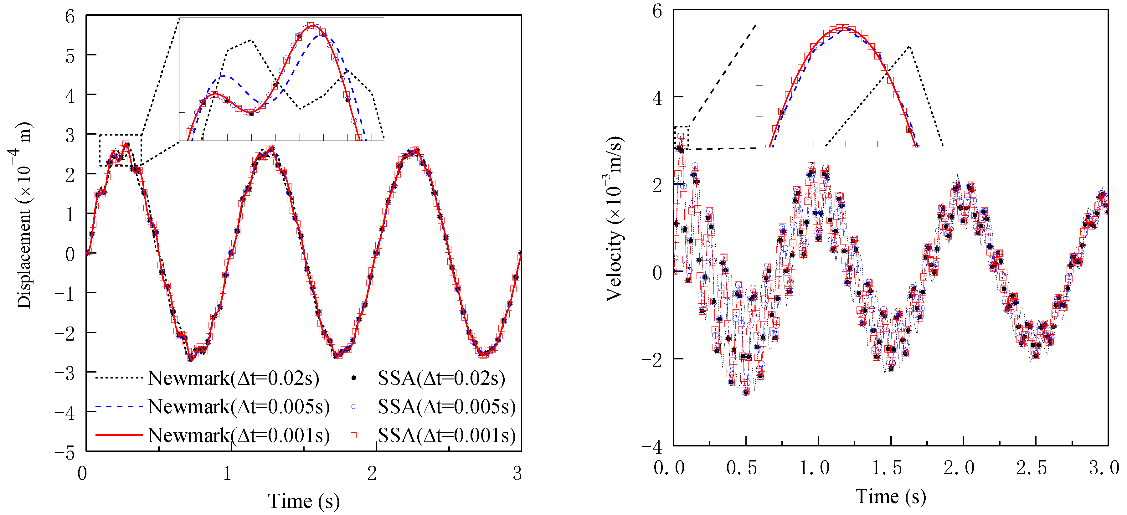
To assess the accuracy of the SSA, the SDOF system under a sinusoidal load was also analyzed using the conventional constant average acceleration Newmark method. Two scenarios were considered for the damping ratio ξ: 0.01 and 1, and the period T was adjusted to 0.1 and 1 s, respectively. The displacement and velocity responses of the SDOF system obtained from both methods were compared and are presented in Figure 3, Figure 4 and Figure 5. The comparison reveals that for SDOF systems with low damping ratios and small periods (or high stiffness), the predictions obtained by the conventional Newmark method are highly sensitive to the time step used. Accurate results that closely match those from the SSA require using an extremely small time step. In contrast, predictions from the SSA are minimally influenced by the time step, demonstrating superior accuracy under these conditions. These findings provide compelling evidence that the SSA surpasses the conventional Newmark method in accuracy, especially for dynamic systems characterized by low damping ratios and high stiffness.

5.2. Fifteen-Storey 3-Bay Plane Frame

5.2.1. FE Model Description

The geometry, load pattern, I-shaped section dimensions, and material model of the 15-storey 3-bay plane steel frame are provided in references [8,29]. Each beam in the frame, shown in Figure 6a, was discretized using 6 displacement-based Euler–Bernoulli beam (DEBE) elements with distributed plasticity, while each column was modeled using 3 DEBE elements. Five Gauss–Legendre integration points were employed in each DEBE element, and the force–deformation relationship at each point was determined using a fiber section model. The I-shaped sections were discretized into 4 layers (i.e., fibers) for the flange and 10 layers (i.e., fibers) for the web. The stress–strain relationship of each discrete fiber followed the uniaxial bilinear constitutive model, incorporating parameters such as Young’s modulus (E), yield strength (f_y), and strain hardening ratio (b). Nodal translational masses were assigned only at the beam–column connections, indicated by black solid circles in Figure 6a. The FE model of the 15-storey frame consisted of 409 nodes and 450 frame elements. All bottom nodes were fully fixed in translational and rotational degrees of freedom (DOFs), resulting in a total of 1215 DOFs for the FE model. The first five periods and circular frequencies of the model are provided in

Table 1. First five periods and angular frequencies in the x direction of the 15-storey plane frame.

Order	1	2	3	4	5
Period (s)	1.25	0.41	0.24	0.17	0.13
Angular frequency (rad/s)	3.41	15.26	26.17	37.22	48.85

.

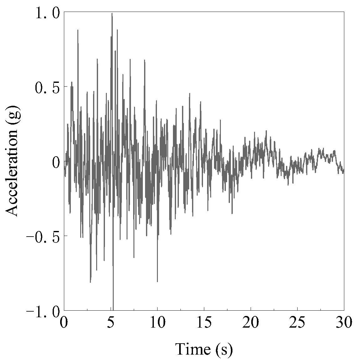
Prior to conducting transient simulations, a gravity analysis was performed on the structure. The gravity load comprised a dead load of 21 N/mm and a live load of 15 N/mm, as depicted in Figure 6a. Convergence criteria were set with a tolerance of 1.0 × 10⁻⁵ mm on the norm of the incremental displacement. For the transient analysis, damping coefficients ξ₁ and ξ₂ were set to 0.2557 and 0.0073, respectively, to achieve a damping ratio of 5% for the first and second modes. The input load for analysis was the 1940 El-Centro wave (see Figure 7). The duration and the time step used for the analysis were 30 s and 0.02 s, respectively.

5.2.2. Comparison between the Employment of CM and LM Matrices

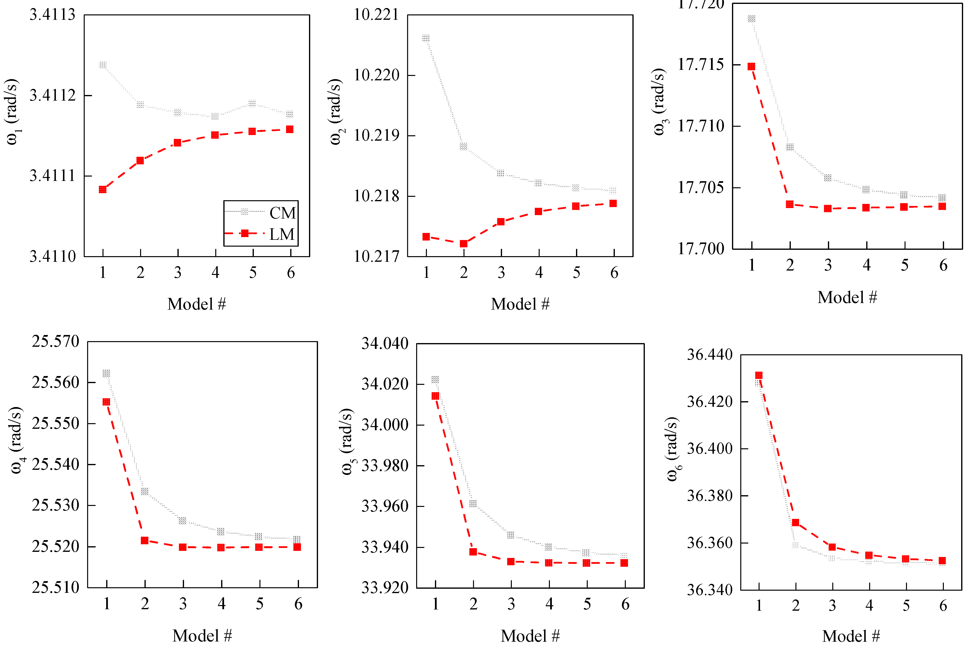
In this section, the numerical results of the frame FE model using the CM and LM matrices were compared. Initially, the angular frequencies were computed. In addition, five more FE models with different mesh were established, designated as Model #1 to #6. These models differ in the number of DEBEs per column and beam. Model #1 has one DEBE per column and two DEBEs per beam, while Model #6 includes six DEBEs per column and twelve DEBEs per beam. Figure 8 presents a comparison of the first six angular frequencies obtained using the CM and LM matrices for these six models. It is evident that regardless of the mass matrix used, the angular frequencies of the first six modes exhibit close proximity to each other.

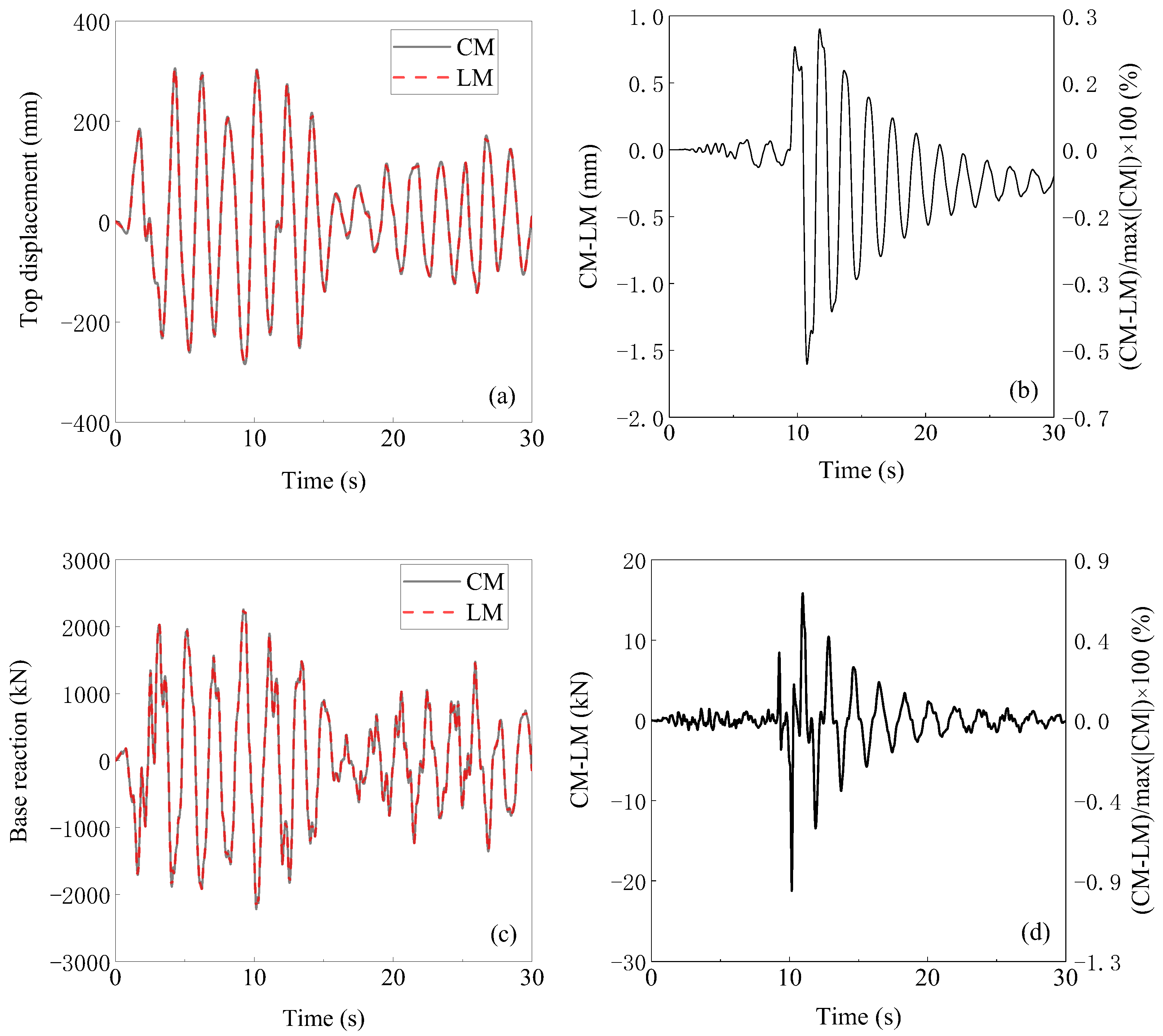
Following this, the FE model depicted in Figure 6 was utilized for seismic analysis. The peak ground accelerations (PGAs) of the earthquake wave were adjusted to 70 and 400 Gal, respectively. Figure 9 and Figure 10 display time history curves of top displacement and base reaction for the frame, respectively, obtained using CM and LM matrices. These figures clearly indicate a high degree of consistency in the predicted global responses from both mass matrices. According to the findings summarized in

Table 2. Computational errors of the plane frame using the two types of mass matrix.

Case (PGA)	Mass Matrix	Method	Max. Top Disp.		Max. Base Reaction		Max. IDR		Disp. RMSE (%)	Reaction RMSE (%)
			Value (mm)	Relative Error (%)	Value (kN)	Relative Error (%)	Value (%)	Relative Error (%)
70	CM	SSA	57.41	--	455.40	--	0.189	--	--	--
	LM	I-SSA	57.41	−0.01	455.32	0.02	0.189	0.00	0.01	0.02
400	CM	SSA	305.52	--	2259.10	--	1.044	--	--	--
	LM	I-SSA	305.50	0.01	2252.25	0.30	1.048	−0.41	0.14	0.13

, the maximum top displacements of the frame predicted using the CM matrix are 57.41 mm and 305.52 mm under the two loading cases, while the corresponding values using the LM matrix are 57.41 mm and 305.50 mm. The relative errors between these predictions are all below 1%. Furthermore, the maximum base reactions are 455.40 kN and 2259.10 kN when using the CM matrix, and 455.32 kN and 2252.25 kN when using the LM matrix, with relative errors of merely 0.02% and 0.30%, respectively.

To quantify the difference between the two time history curves, a root-mean-square error (RMSE) is employed here, which is defined as follows:

$$e_{RMS}=\sqrt{{\displaystyle \frac{1}{N}}\times {\sum }_{i=1}^N{\left(X_i-Y_i\right)}^2}/\mathit{max}\left(\left|X_i\right|\right)\times 100\%,$$

(25)

where N is the number of time steps, and X_i and Y_i are the two responses to be compared. As depicted in Table 2, the RMSEs between the top displacement time histories using the CM and LM matrices under the two cases are 0.01% and 0.14%, respectively, and those between the base reaction time histories are 0.02% and 0.13%, respectively. These low RMSE values indicate very small differences between the time history responses predicted by the CM and LM matrices.

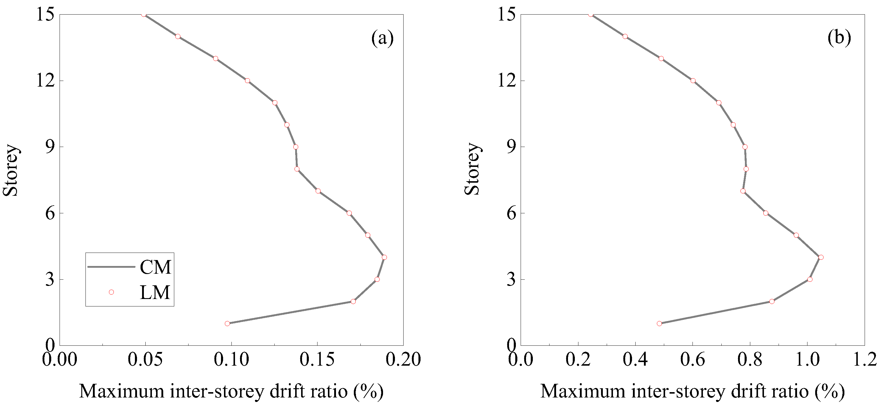
Furthermore, the maximum inter-storey drift ratio (IDR) envelopes of the 15-storey frame, obtained using the CM and LM matrices, are presented in Figure 11 for the two loading cases. It can be observed from the figure that the maximum IDR envelopes of the frame obtained using the CM and LM matrices closely align under both loading cases. As indicated in Table 2, the relative errors between the maximum IDRs obtained using the CM and LM matrices are 0.00% and 0.41%, respectively.

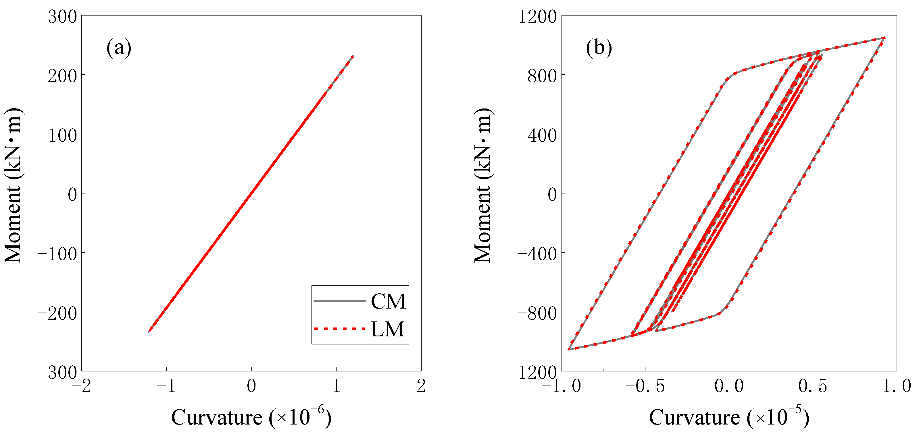
In the final analysis, the local moment–curvature curves of section A-A of the frame depicted in Figure 6 were compared using the CM and LM matrices, as shown in Figure 12 for the two loading cases. The simulation results reveal that regardless of the mass matrix employed, the local responses exhibit a high degree of similarity.

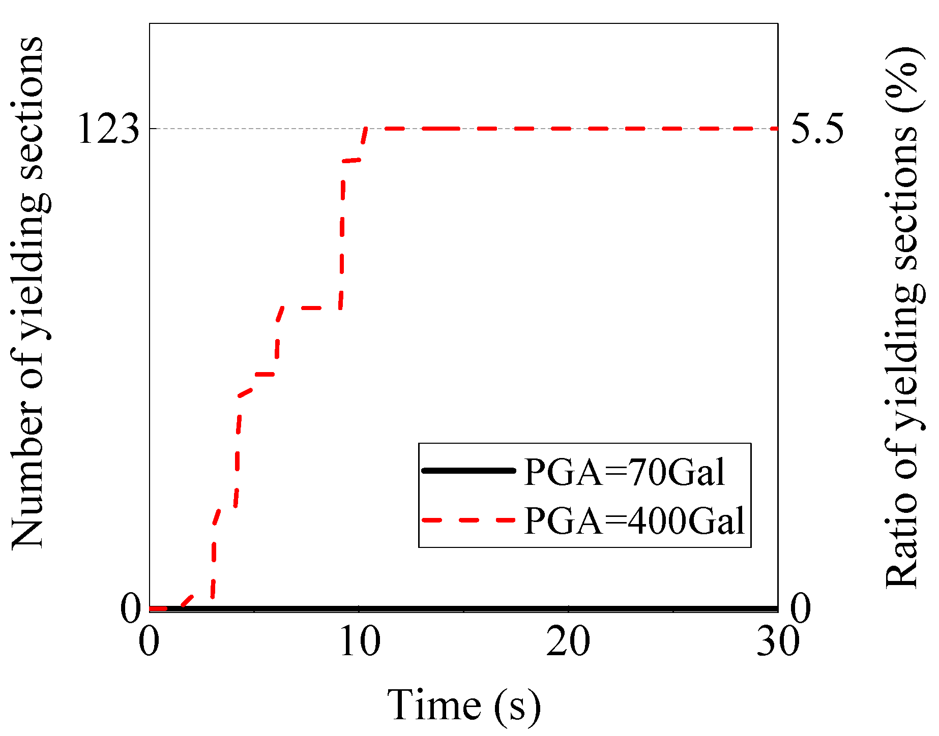
Figure 13 presents the number of yielding sections in the frame under the same two loading cases. In the first loading case, no sections yield, indicating that the structure remains in a linear elastic state. This observation is crucial in understanding why the I-SSA yields similar numerical results to the conventional Newmark method. However, in the second loading case, a total of 123 sections yield, which corresponds to approximately 5.5% of the sections undergoing nonlinear behavior. Based on the comprehensive analysis conducted, it is concluded that the numerical results obtained from the FE model using the LM matrix demonstrate a high level of consistency with those obtained using the CM matrix. Therefore, for subsequent analyses, the LM matrix will be employed.

5.2.3. Study of Numerical Accuracy

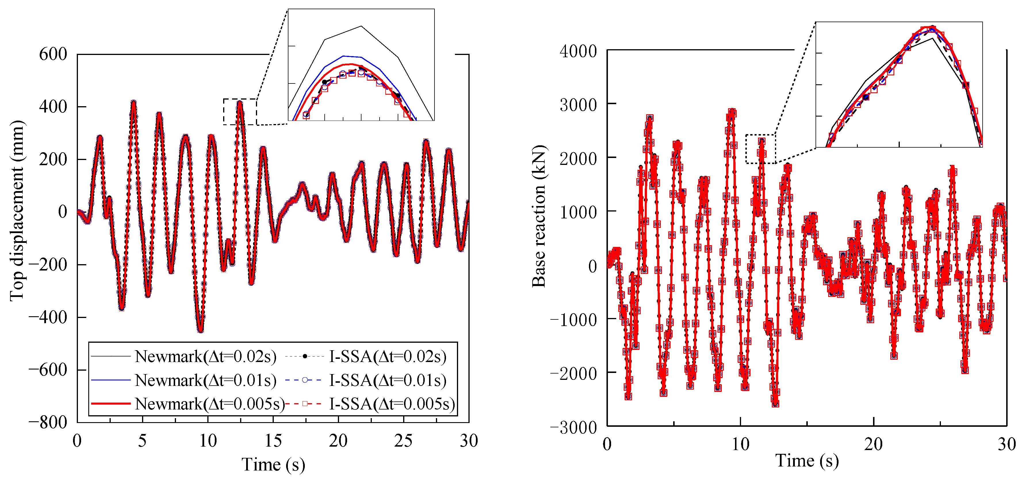
In this section, the numerical accuracy of the 15-storey frame using the I-SSA was investigated. The seismic analysis of the same frame FE model was also conducted using the conventional Newmark method for comparison. Figure 14 illustrates the global responses of the frame under the El-Centro earthquake wave with the PGA of 620 Gal, using different time steps of 0.02, 0.01, and 0.005 s. The figure clearly shows that regardless of the time step used, the top displacement and base reaction time histories as well as the maximum IDR envelopes (see Figure 15) obtained from both methods exhibit a high degree of similarity. However, it is important to note that the global response predicted by the Newmark method shows a slight sensitivity to the chosen time step. This sensitivity suggests that smaller time steps may be required to achieve more accurate predictions of dynamic responses, particularly when capturing detailed transient effects or highly nonlinear behavior of the structure.

The computational errors of both methods under the three different time steps are presented in

Table 3. Computational errors between the Newmark and I-SSA under the three time steps.

Time Step (s)	Method	Max. Top Disp.		Max. Base Reaction		Max. IDR		Disp. RMSE (%)	Reaction RMSE (%)
		Value (mm)	Relative Error (%)	Value (kN)	Relative Error (%)	Value (%)	Relative Error (%)
0.02	Newmark	450.12	0.77	2874.6	0.27	1.823	1.10	0.52	0.74
	I-SSA	452.75		2882.3		1.845
0.01	Newmark	449.85	0.80	2880.3	−0.02	1.822	1.09	0.52	0.49
	I-SSA	452.46		2879.7		1.845
0.005	Newmark	449.82	0.81	2881.1	−0.07	1.822	1.11	0.53	0.49
	I-SSA	452.44		2879.0		1.845

. The relative errors of the maximum top displacement are 0.3%, 0.2%, and 0.1% for the three time steps. Similarly, the relative errors of the maximum base reactions are 0.3%, 0.1%, and 0.3%, while the relative errors of the maximum IDRs are 0.00%, 0.00%, and 0.10%. These results indicate that the RMSEs of the top displacement and base reaction are all very small and exhibit minimal sensitivity to the intensity of the ground motion. This suggests a high level of accuracy and consistency in the numerical predictions of both methods in this specific application, regardless of the chosen time step.

5.2.4. Influence of Mass Distribution

In this section, the impact of mass distribution on accuracy and efficiency was examined. This section considered four different mass matrices: (1) CM, (2) lumped masses assigned at each nodal translational DOF (LM1), (3) lumped masses assigned at each beam–column joint nodal translational DOF (LM2), and (4) lumped masses assigned at the translational DOF of the mid-node in each floor (LM3). In the three LM matrices, nodal rotational inertias were neglected, while the total structural masses were kept consistent.

Table 4. Computational results of four different mass matrices.

Case (PGA)	Mass Matrix	Top Disp.		Base Reaction		Max. IDR		Disp. RMSE (%)	Reaction RMSE (%)
		Max. (mm)	Error (%)	Max. (kN)	Error (%)	Max. (%)	Error (%)
70	CM	57.41	--	455.40	--	0.19	--	--	--
	LM1	57.41	−0.01	455.32	0.02	0.19	−0.00	0.01	0.02
	LM2	57.43	−0.04	455.51	−0.02	0.19	−0.02	0.03	0.09
	LM3	57.45	−0.07	455.52	−0.03	0.19	0.03	0.07	0.22
400	CM	305.52	--	2259.10	--	1.04	--	--	--
	LM1	305.50	0.01	2252.30	0.30	1.05	−0.41	0.14	0.13
	LM2	305.48	0.02	2244.55	0.64	1.05	−0.77	0.26	0.27
	LM3	305.33	0.06	2246.74	0.55	1.05	−0.74	0.29	0.35
620	CM	450.26	--	2883.61	--	1.82	--	--	--
	LM1	452.75	−0.55	2882.28	0.05	1.85	−1.27	0.54	0.50
	LM2	455.32	−1.13	2893.95	−0.36	1.86	−2.29	0.97	0.92
	LM3	454.97	−1.05	2890.11	−0.23	1.86	−2.33	1.03	1.00

presents the computational results obtained using the I-SSA with these four different mass matrices. The CM matrix represents the most theoretically rigorous choice, and its numerical results are considered as the accurate benchmark. It is evident from Table 4 that the simulation predictions using the three lumped mass matrices (i.e., LM1, LM2, and LM3) are highly consistent with those obtained from the CM matrix. It indicates that the seismic response of the frame FE model is not significantly influenced by the specific mass matrix employed in this example.

Finally, the computational results of the four mass matrices are compared in

Table 5. Sizes of mass and transition matrices using different mass matrix types.

Mass Matrix Type	CM	LM1	LM2	LM3
Sizes of mass matrix	1215 × 1215	810 × 810	120 × 120	30 × 30
Sizes of transition matrix	2430 × 2430	1620 × 1620	240 × 240	60 × 60

. When using the consistent element mass matrix, the dimensions of the structural mass matrix M and the transition matrix A are 1215 × 1215 and 2430 × 2430, respectively. In contrast, the effective structural mass matrix M₁ and the corresponding transition matrix $\overline{\mathit{A}}$ are significantly reduced when employing the lumped element mass matrix. In the three LM matrices, the dimensions of the effective structural mass matrix M₁ are 810, 120, and 30, respectively, resulting in the transition matrices $\overline{\mathit{A}}$’s dimensionalities of 1620, 240, and 60, respectively. Theoretically, the computational time per iteration is expected to decrease when the size of the transition matrix $\overline{\mathit{A}}$ becomes smaller. However, in this particular example, the computational efficiency benefits of lumped element mass matrices are not evident due to the relatively small number of DOFs in the plane frame.

5.3. Fifteen-Storey Frame Equipped with LVDs

In Figure 6b, the 15-storey 3-bay frame previously mentioned was retrofitted with LVDs installed at the mid-span locations. In the FE model, each LVD was represented by a truss element and a uniaxial viscous material. The loading cases used in the previous analysis were also applied here. Both the proposed I-SSA and the Newmark method were employed to conduct nonlinear time history analysis of the LVD-equipped frame.

5.3.1. Investigation of Accuracy

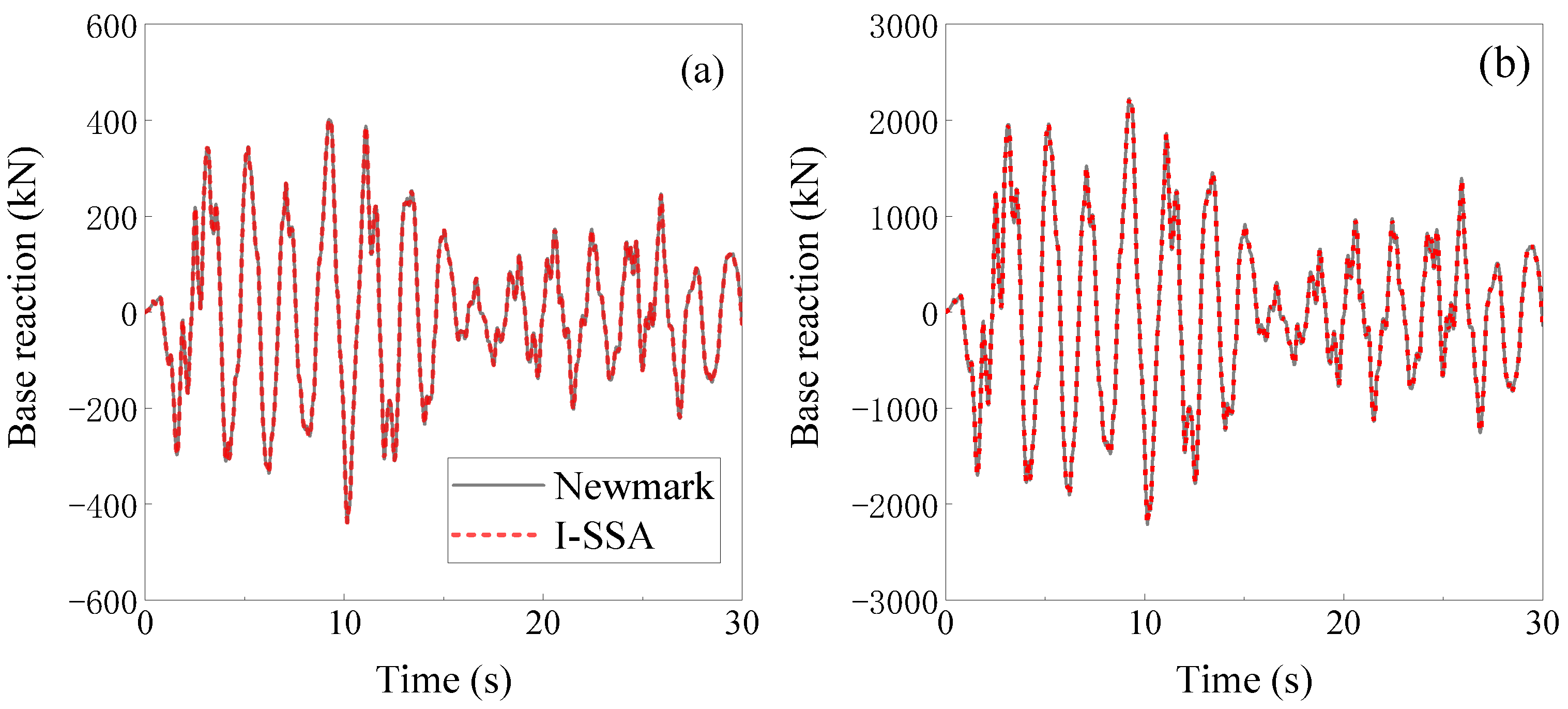
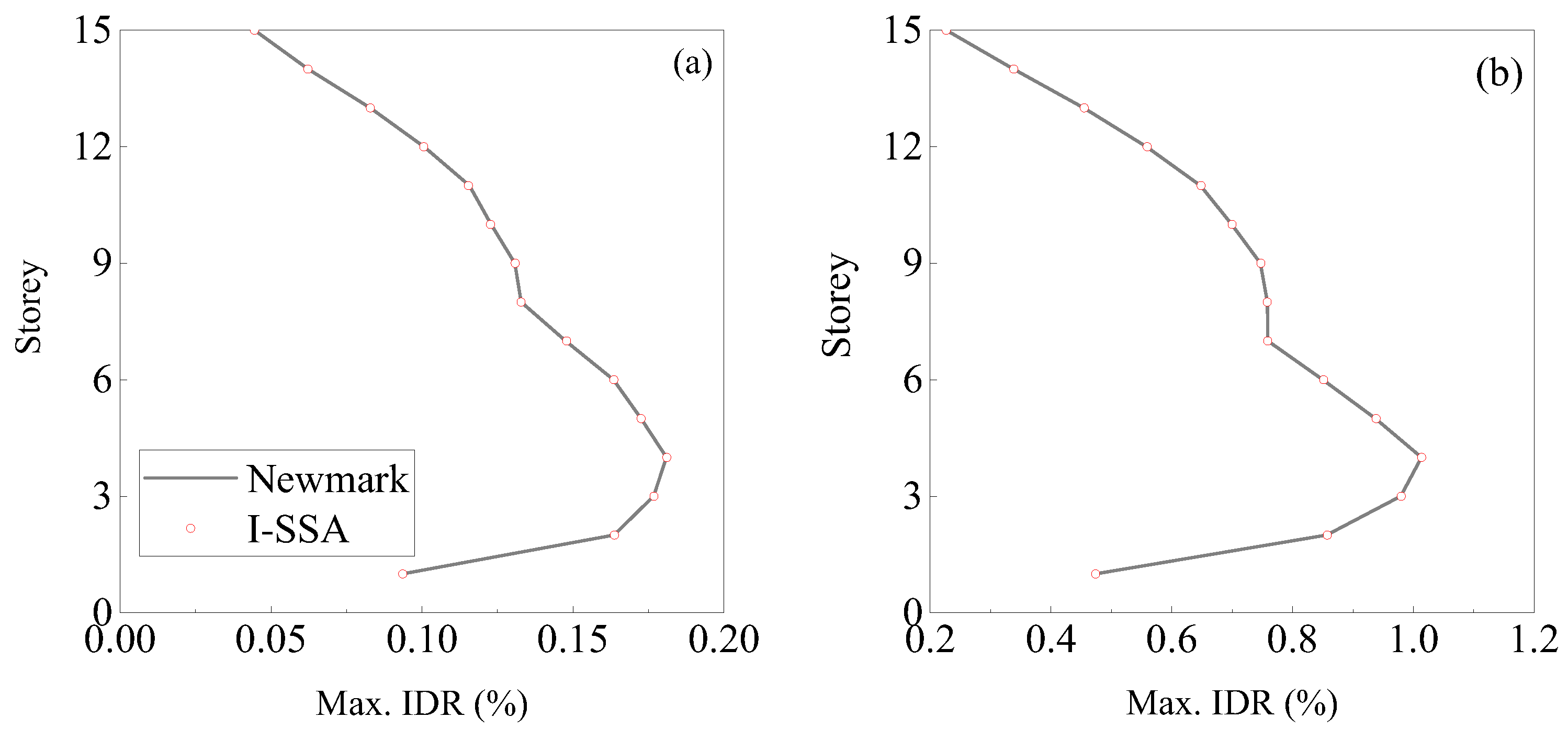
The damping coefficient c of the LVD was set to 0.2 kN/(mm/s). Figure 16, Figure 17 and Figure 18 illustrate the time history curves of the top displacement, base reaction, and maximum IDRs of the frame, respectively. Additionally, Figure 19 compares the relationship between axial force and strain of LVD #5. These figures clearly indicate that the global and local responses of the LVD-equipped frame obtained from both the I-SSA and Newmark method are nearly identical.

Since the results obtained by the I-SSA are almost identical to those obtained by the Newmark method, and the previous validation shows that the calculation accuracy of the I-SSA remains unaffected despite variations in the time step values, the I-SSA will be used in the following numerical examples to achieve equivalent accuracy with significantly fewer calculation steps than Newmark, resulting in fast and efficient calculations.

5.3.2. Effect of the Damping Coefficient of LVDs on Structural Response

Table 6. Responses and errors of the frame equipped with LVDs of various damping coefficients.

c (kN/(mm/s))	Top Disp.		Top Vel.
	Max. Value (mm)	Relative Error	Max. Value (mm/s)	Relative Error
0.00	305.33	--	1271.58	--
0.50	294.79	3.45%	1192.61	6.21%
1.00	282.21	7.57%	1130.95	11.06%
c (kN/(mm/s))	Base Reaction		Max. IDR
	Max. Value (kN)	Relative Error	Max. Value (%)	Relative Error
0.00	2246.74	--	1.05	--
0.50	2169.30	3.45%	0.97	7.62%
1.00	2105.61	6.28%	0.89	15.17%

illustrates responses and errors of the 15-storey frame equipped with LVDs of various damping coefficients subjected to the El-Centro earthquake wave with the PGA of 400 Gal. The damping coefficients c of each LVD were assumed to be 0.00, 0.50, and 1.00 kN/(mm/s), respectively. The analysis indicates notable reductions in maximum displacements, maximum velocities, base reactions, and maximum IDRs following LVD installation. Moreover, higher damping coefficients for LVDs demonstrate enhanced mitigation of structural response to seismic forces. Thus, the strategic installation of LVDs with appropriate damping coefficients proves effective in seismic response mitigation.

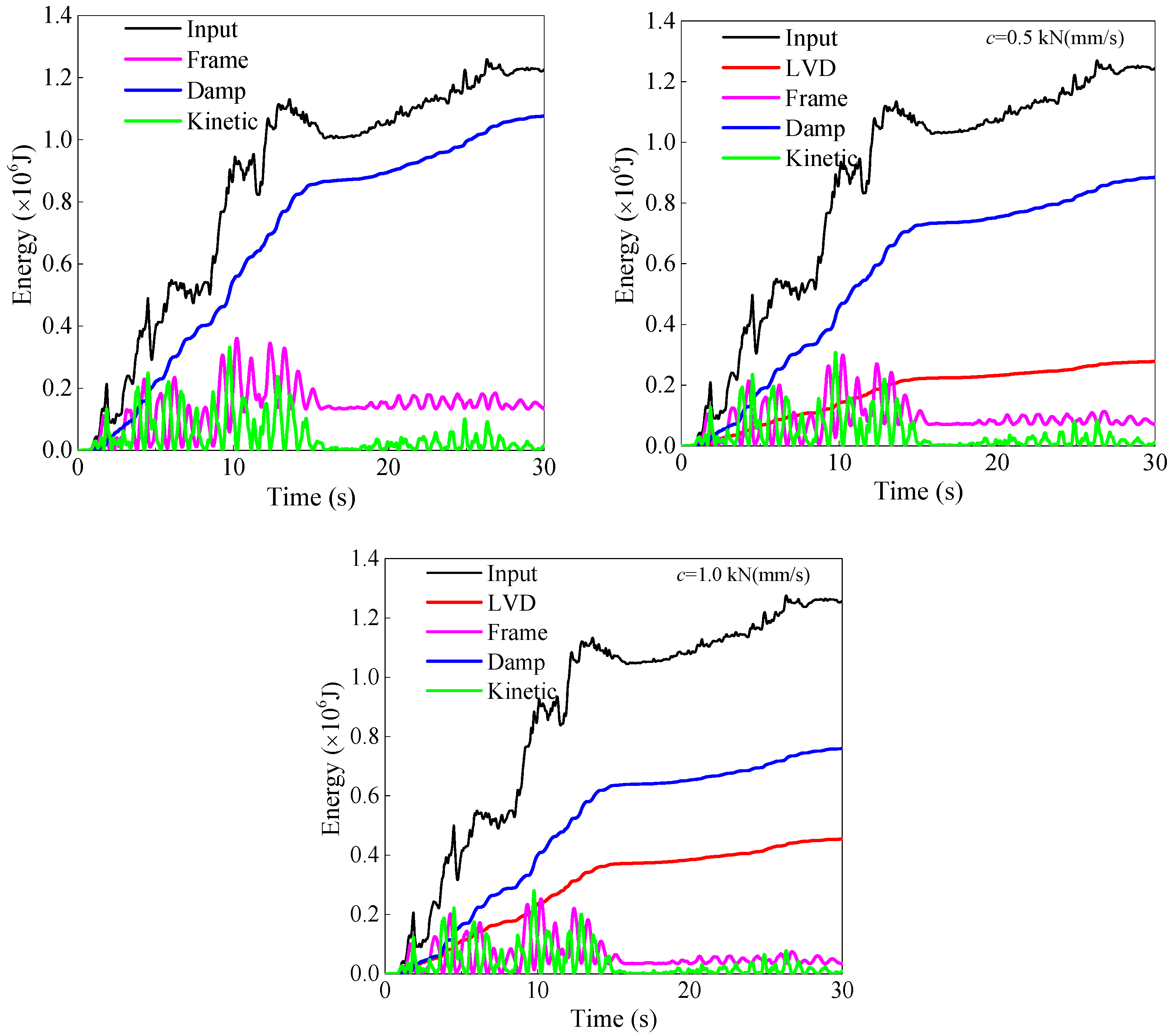
Figure 20 shows energy dissipations of the frame equipped with LVDs of various damping coefficients. In this numerical example, the seismic input energy of the frame is mainly dissipated by the structural damping. As the damping coefficient of the LVD increases, the energy dissipated by the LVD increases and the energy dissipated by the structural damping decreases dramatically, and the energy absorbed by the frame elements is also reduced.

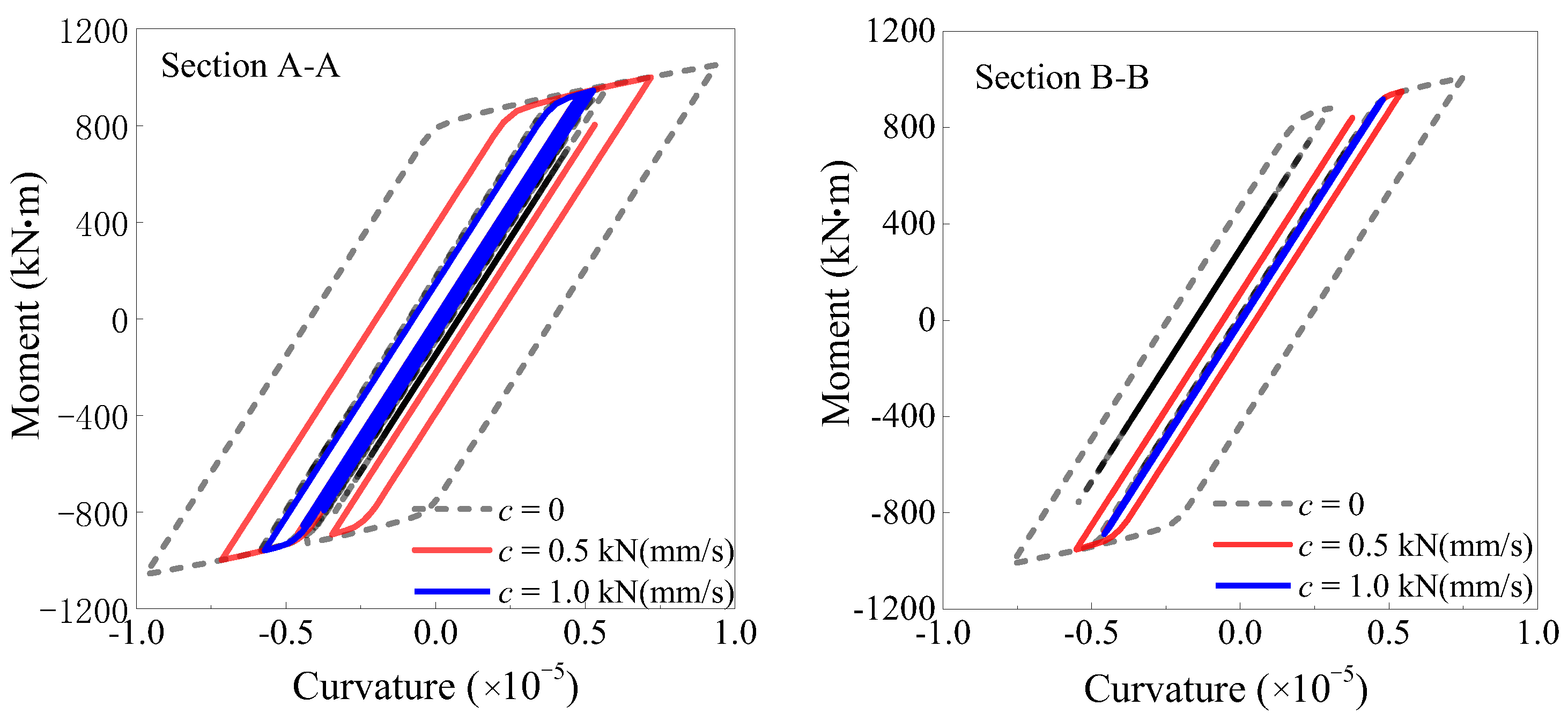
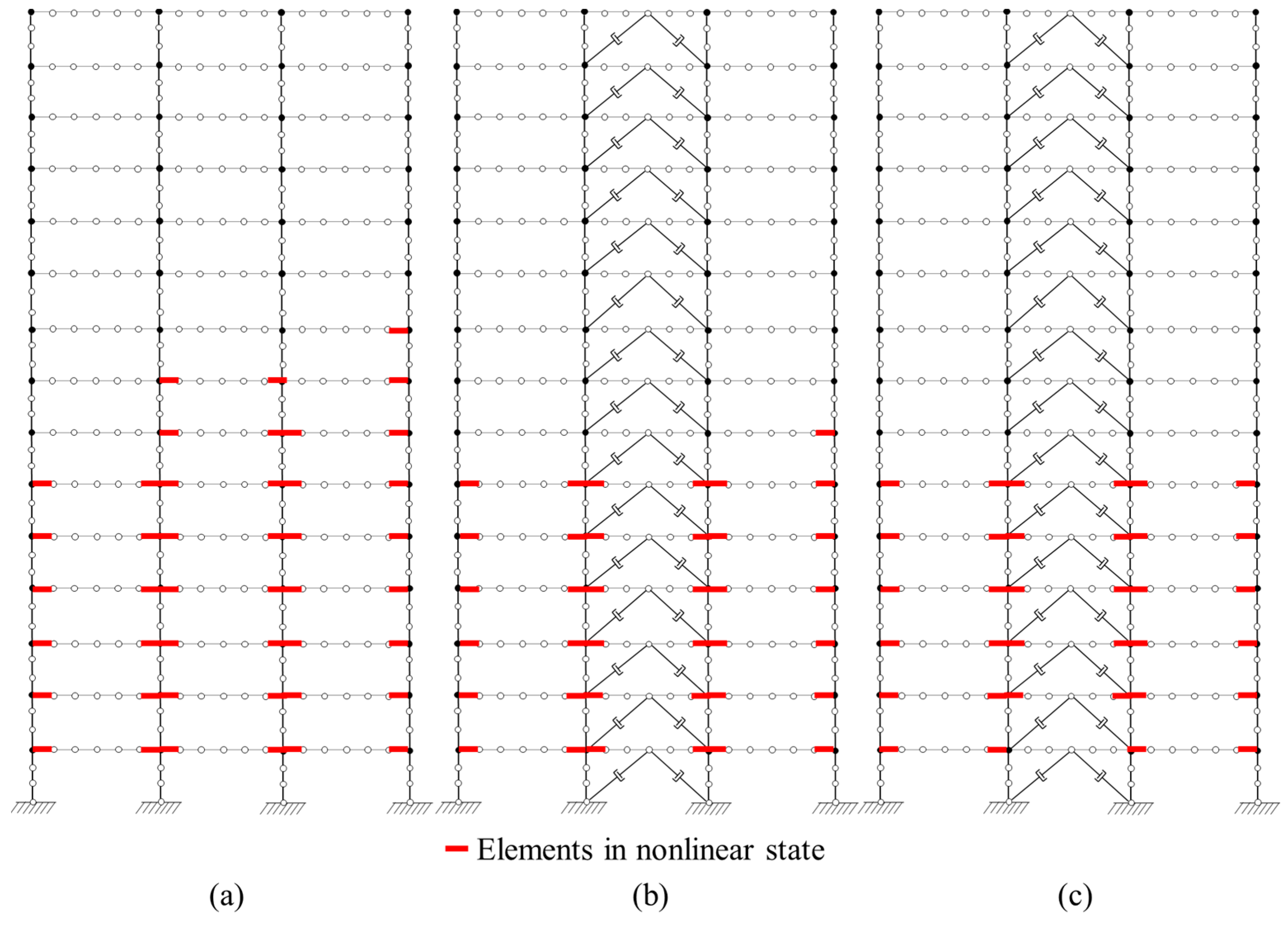
A comparative analysis of the moment–curvature curves at sections A-A and B-B demonstrates significant attenuation following the installation of LVDs in Figure 21. A substantial portion of energy dissipation previously controlled by hysteresis is now absorbed by the LVDs, thereby reducing the plastic energy dissipation in the beams and enhancing structural safety. Additionally, LVDs dissipate more energy as the damping coefficient increases, further mitigating frame hysteresis. As shown in Figure 22, the white circles are nodes without assigned lumped mass and the black circles are nodes with assigned lumped mass, it compares the nonlinear element distribution of the frame equipped with LVDs of different damping coefficients. When the damping coefficient increases from zero to 1.0 kN(mm/s), the number of yielding elements decreases from 44 to 33. Obviously, the energy dissipated by the LVDs results in a reduction in the total structural plastic energy dissipation, allowing more elements to remain in the linear elastic state.

6. Conclusions

This study introduces an improved state-space approach (I-SSA) utilizing a lumped mass matrix for transient analysis of structures. Three numerical examples are provided, and the key conclusions are summarized as follows:

(1)

The SSA exhibits superior accuracy and stability compared to conventional step-by-step integration methods, such as the Newmark method, especially for systems with low damping ratios and high stiffness. In linear single-degree-of-freedom systems with small damping ratios and periods, the Newmark method exhibits higher sensitivity to the time step, whereas the SSA is more robust.

(2)

The choice of mass matrix has a negligible impact on the simulation predictions of the I-SSA. For instance, in the case of the 15-storey plane steel frame, the angular frequency, global, and local responses computed using the lumped mass (LM) matrix closely align with those obtained using the consistent mass (CM) matrix. Simultaneously, numerical simulations using various LM matrices yield highly similar results. Under PGAs of 70, 400, and 620 Gal, the relative errors when using an LM matrix compared to the CM matrix are 1.13% for the maximum top displacement, 0.36% for the maximum base reaction, and 2.33% for the maximum IDR. Additionally, the root-mean-square errors for top displacement and base reaction time histories are generally less than 1%, indicating that the simulation predictions using the LM matrices are highly consistent with those obtained from the CM matrix.

(3)

The use of the LM matrix can significantly reduce the dimensionality of the governing equation in the I-SSA. Unlike the CM matrix, which results in a full-rank structural mass matrix and a state-space equation dimension twice that of the structural degrees of freedom, the LM-based approach assigns zero masses to many nodes (or degrees of freedom), effectively reducing the effective dimensions of the equation. The numerical results in this study demonstrate that the simulation outcomes for the 15-storey plane steel frame using an LM mass matrix of size 30 × 30, which significantly reduces the dimensionality of the control equations, are nearly identical to those obtained using a CM matrix of size 1215 × 1215.

(4)

The LM-based I-SSA shows promising theoretical efficiency and substantial potential for dynamic analysis of large-scale structures. By reducing the computational complexity through the LM matrix, the method offers efficient analysis capabilities for extensive structural systems.

In conclusion, the I-SSA with a lumped mass matrix not only enhances accuracy and stability in transient structural analysis but also facilitates computational efficiency, particularly for complex and large-scale structures. These advantages position the method as a valuable tool for engineers and researchers engaged in dynamic analysis and seismic assessment of buildings and infrastructure.

References

1. Wu, B.; Bao, H.; Ou, J.; Tian, S. Stability and accuracy analysis of the central difference method for real-time substructure testing. Earthq. Eng. Struct. Dyn. 2005, 34, 705–718. [Google Scholar] [CrossRef]
2. Akbar Gholampour, A.; Ghassemieh, M.; Karimi-Rad, M. A new unconditionally stable time integration method for analysis of nonlinear structural dynamics. J. Appl. Mech. 2013, 80, 021024. [Google Scholar] [CrossRef]
3. Ozkul, T.A. A finite element formulation for dynamic analysis of shells of general shape by using the Wilson-θ method. Thin-Walled Struct. 2004, 42, 497–513. [Google Scholar] [CrossRef]
4. Kim, W. Improved two-stage implicit time integration methods with unconventionally determined parameters for analyses of linear and nonlinear structural dynamics. Nonlinear Dyn. 2024, 112, 1221–1259. [Google Scholar] [CrossRef]
5. Mosqueda, G.; Ahmadizadeh, M. Iterative implicit integration procedure for hybrid simulation of large nonlinear structures. Earthq. Eng. Struct. Dyn. 2011, 40, 945–960. [Google Scholar] [CrossRef]
6. Jain, S.; Tiso, P.; Rutzmoser, J.B.; Rixen, D.J. A quadratic manifold for model order reduction of nonlinear structural dynamics. Comput. Struct. 2017, 188, 80–94. [Google Scholar] [CrossRef]
7. Amini, A.M.; Dureisseix, D.; Cartraud, P. Multi-Scale domain decomposition method for large-scale structural analysis with a zooming technique: Application to plate assembly. Int. J. Numer. Methods Eng. 2009, 79, 417–443. [Google Scholar] [CrossRef]
8. Sun, B.; Zeng, Z.; Sun, T.; Shen, W.; Ou, J. An efficient reduced-order multi-scale simulation approach for nonlinear analysis of frame structures with nonlinear localization. J. Earthq. Eng. 2024, 28, 325–348. [Google Scholar] [CrossRef]
9. Lopez Almansa, F.; Barbat, A.H.; Rodellar, J. SSP algorithm for linear and non-linear dynamic response simulation. Int. J. Numer. Methods Eng. 1988, 26, 2687–2706. [Google Scholar] [CrossRef]
10. Xu, L.; Zhai, W.; Zhu, S.; Liu, W. An efficient method for train–track–substructure dynamic interaction analysis by implicit-explicit integration and multi-time-step solution. Railw. Eng. Sci. 2023, 31, 20–36. [Google Scholar] [CrossRef]
11. Clough, R.W.; Penzien, J.; Griffin, D.S. Dynamics of Structures; Computers & Structures, Inc.: Berkeley, CA, USA, 1993. [Google Scholar]
12. Zhang, J.; Liu, Y.; Liu, D. Accuracy of a composite implicit time integration scheme for structural dynamics. Int. J. Numer. Methods Eng. 2017, 109, 368–406. [Google Scholar] [CrossRef]
13. Fritzen, P.; Wittekindt, J. Numerical solution of viscoplastic constitutive equations with internal state variables Part I: Algorithms and implementation. Math. Method Appl. Sci. 1997, 20, 1411–1425. [Google Scholar] [CrossRef]
14. Simeonov, V.K.; Sivaselvan, M.V.; Reinhorn, A.M. Nonlinear analysis of structural frame systems by the state-space approach. Comput. Aided Civ. Infrastruct. Eng. 2000, 15, 76–89. [Google Scholar] [CrossRef]
15. Wang, Y.; Liao, W.; Lee, C. A state-space approach for dynamic analysis of sliding structures. Eng. Struct. 2001, 23, 790–801. [Google Scholar] [CrossRef]
16. Sivaselvan, M.V.; Reinhorn, A.M. Collapse analysis: Large inelastic deformations analysis of planar frames. J. Struct. Eng. 2002, 128, 1575–1583. [Google Scholar] [CrossRef]
17. Sivaselvan M, V. Nonlinear Structural Analysis towards Collapse Simulation: A Dynamical Systems Approach; State University of New York at Buffalo: Buffalo, NY, USA, 2003; pp. 27–41. [Google Scholar]
18. Lu, L.; Chung, L.; Wu, L.; Lin, G. Dynamic analysis of structures with friction devices using discrete-time state-space formulation. Comput. Struct. 2006, 84, 1049–1071. [Google Scholar] [CrossRef]
19. Kildashti, K.; Mirghaderi, R. Assessment of seismic behaviour of SMRFs with RBS connections by means of mixed-based state-space approach. Struct. Des. Tall Spec. Build. 2009, 18, 485–505. [Google Scholar] [CrossRef]
20. Jafari, V.; Rahimian, M.; Vahdani, S.H. Improved formulation in mixed-based state-space approach for large displacement inelastic analysis of frames. J. Eng. Mech. 2011, 137, 196–204. [Google Scholar] [CrossRef]
21. Amir, M.; Papakonstantinou, K.G.; Warn, G.P. State-Space Formulation for Structural Analysis with Coupled Degradation-Plasticity and Geometric Nonlinearity. J. Struct. Eng. 2022, 148, 04022016. [Google Scholar] [CrossRef]
22. Liu, X.; Wang, Y.; Wang, G.; Yang, B.; Xu, R. Dynamic analysis of RC beams externally bonded with FRP plates using state space method. Eng. Struct. 2022, 253, 113788. [Google Scholar] [CrossRef]
23. Trujillo, D.M. The direct numerical integration of linear matrix differential equations using Padé approximations. Int. J. Numer. Methods Eng. 1975, 9, 259–270. [Google Scholar] [CrossRef]
24. Rodellar, J.; Barbat, A.H. Numerical analysis of the seismic response. A state space approach. In Proceedings of the NUMETA’85 Conference, Swansea, UK, 7–11 January 1985; pp. 273–279. [Google Scholar]
25. Wan-Xie, Z. On precise integration method. J. Comput. Appl. Math. 2004, 163, 59–78. [Google Scholar] [CrossRef]
26. Simo, J.C.; Hughes, T.J.R. Computational Inelasticity; Springer: Berlin/Heidelberg, Germany, 1998. [Google Scholar]
27. Yang, J.B.; Jiang, L.J.; Chen, D.C.H. Dynamic modelling and control of a rotating Euler–Bernoulli beam. J. Sound Vib. 2004, 274, 863–875. [Google Scholar] [CrossRef]
28. Naeim, F. Dynamics of structures-theory and applications to earthquake engineering. Earthq. Spectra 2007, 23, 491–492. [Google Scholar] [CrossRef]
29. Sun, B.; Zeng, Z.; Zhang, Y.; Shen, W.; Ou, J. An effective geometric nonlinear analysis approach of framed structures with local material nonlinearities based on the reduced-order Newton-Raphson method. Soil Dyn. Earthq. Eng. 2023, 172, 107991. [Google Scholar] [CrossRef]
Figure 1. Analytical flowchart of the I-SSA.
Buildings 14 02735 g001
Figure 2. SDOF mass–spring damping system under sinusoidal load.
Buildings 14 02735 g002
Figure 3. Displacement and velocity responses of the SDOF system (ω = 0.01 and T = 0.1 s).
Buildings 14 02735 g003
Figure 4. Displacement and velocity responses of the SDOF system (ω = 1 and T = 0.1 s).
Buildings 14 02735 g004
Figure 5. Displacement and velocity responses of the SDOF system (ω = 0.01 and T = 1 s).
Buildings 14 02735 g005
Figure 6. Fifteen-story plane steel frame (a) without LVDs and (b) equipped with LVDs.
Buildings 14 02735 g006
Figure 7. Normalized 1940 El-Centro earthquake wave.
Buildings 14 02735 g007
Figure 8. Comparisons of first six angular frequencies of the six models using the two mass matrices.
Buildings 14 02735 g008
Figure 9. Comparisons of response time history curves of the CM and LM matrices and their discrepancies under the earthquake motion of 70 PGA: (a) top disp. response, (b) top disp. discrepancy, (c) base reaction response, (d) base reaction relative error.
Buildings 14 02735 g009
Figure 10. Comparisons of response time history curves of the CM and LM matrices and their discrepancies under the earthquake motion of 400 PGA: (a) top disp. response, (b) top disp. discrepancy, (c) base reaction response, (d) base reaction relative error.
Buildings 14 02735 g010
Figure 11. Maximum IDR envelopes of the 15-storey frame using the two mass matrices: (a) PGA = 70 Gal, (b) PGA = 400 Gal.
Buildings 14 02735 g011
Figure 12. Comparisons of moment–curvature curves of section A-A using the CM and LM matrices: (a) PGA = 70 Gal, (b) PGA = 400 Gal.
Buildings 14 02735 g012
Figure 13. Number and ratio of yielding elements time history curves under the three loading cases.
Buildings 14 02735 g013
Figure 14. Top displacement and base reaction time history curves of the plane frame obtained from the Newmark and I-SSA using three different time steps.
Buildings 14 02735 g014
Figure 15. Maximum IDR envelopes of the 15-storey frame predicted by the Newmark and I-SSA using three different time steps.
Buildings 14 02735 g015
Figure 16. Top displacement time history curves of the frame equipped with LVDs obtained from the Newmark and I-SSA: (a) PGA = 70 Gal, (b) PGA = 400 Gal.
Buildings 14 02735 g016
Figure 17. Base reaction time history curves of the frame equipped with LVDs using the Newmark and I-SSA: (a) PGA = 70 Gal, (b) PGA = 400 Gal.
Buildings 14 02735 g017
Figure 18. Maximum IDR envelopes of the frame equipped with LVDs using the Newmark and I-SSA: (a) PGA = 70 Gal, (b) PGA = 400 Gal.
Buildings 14 02735 g018
Figure 19. Axial force vs. strain curves of the LVD #5 predicted by the Newmark and I-SSA: (a) PGA = 70 Gal, (b) PGA = 400 Gal.
Buildings 14 02735 g019
Figure 20. Energy dissipation of the frame equipped with LVDs of various damping coefficients.
Buildings 14 02735 g020
Figure 21. Comparisons of sectional moment–curvature curves.
Buildings 14 02735 g021
Figure 22. Yielding elements distribution of the frame equipped with LVDs of various damping coefficients: (a) c = 0, (b) c = 0.5 kN/(mm/s), (c) c = 1.0 kN/(mm/s).
Buildings 14 02735 g022