Energy-Saving Optimization of HVAC Systems Using an Ant Lion Optimizer with Enhancements

Abstract

The complex and time-varying external climate conditions and multi-equipment variable coupling characteristics make it challenging to optimize the Heating, Ventilation, and Air Conditioning (HVAC) systems in existing buildings effectively. Additionally, the intricate energy exchange processes within HVAC systems present difficulties in developing accurate and generalizable energy consumption models. In response to these challenges, this paper proposes an Ant Lion Optimizer with Enhancements (ALOE) that can dynamically adjust the number of populations and the movement trend to improve the convergence speed and optimization ability, and randomly adjust the movement amplitude to enhance the local optimal escape ability. Finally, a case study of an office building in Hangzhou was carried out, and an overall energy consumption model of the HVAC system based on parameter identification and a general mechanism model was established. In this model, the energy-saving optimization effects of various advanced swarm intelligence optimization algorithms were compared. The experimental results demonstrate that under high, medium, and low load conditions, the ALOE algorithm achieves energy-saving rates of 28.16%, 28.26%, and 24.85%, respectively, the overall energy-saving rate for the entire day reaches 29.06%, which indicates the ALOE has significant superiority. This work will contribute to the development of energy-saving and emission-reduction technologies.

1. Introduction

1.1. Background

With the rapid development of the social economy, energy demand and carbon emissions have been rising annually, exacerbating global energy shortages and environmental pollution issues. According to the “2022 China Building Energy Consumption and Carbon Emission Research Report” [1], in 2020, the total energy consumption over the entire life cycle of buildings in China reached 2.27 billion tons of standard coal equivalent, accounting for 45.5% of energy consumption of the nation. The corresponding carbon emissions amounted to 5.08 billion tons of carbon dioxide, representing 50.9% of the carbon emissions of the republic. Among the various components of building energy consumption, HVAC systems account for the highest proportion, about 40% to 60% of the total building energy consumption [2]. Currently, the energy management of existing buildings primarily relies on manual experience, making it challenging to quickly and accurately adapt to dynamic changes in cooling loads, leading to low system operational efficiency [3]. Therefore, conducting energy-saving optimization research on HVAC systems is crucial, as it can significantly enhance system efficiency and greatly reduce energy consumption and carbon emissions.

1.2. Literature Review

Establishing accurate system models is an indispensable part of energy-saving optimization research for HVAC systems. The commonly used modeling methods can be broadly categorized into mechanistic modeling and data-driven modeling. Mechanistic modeling methods build precise mathematical models based on the actual characteristics and operating mechanisms of the target system. For instance, Kohlenbach et al. [4] developed a dynamic model of an absorption chiller based on internal energy and material balance, demonstrating good consistency between simulation and experimental results. Wemhoff et al. [5] conducted a comprehensive analysis of an air conditioning system, utilizing a nonlinear implicit solution algorithm to perform steady-state and transient calculations of flow resistance, water mass balance, and energy conservation, thereby achieving the coupling of fluid transport, energy transfer, thermodynamics, and humidity. Vakiloroaya et al. [6] modeled a cooling tower using the effectiveness-NTU method, incorporating physical variables such as air quality flow rate and ambient air enthalpy. Park et al. [7] calculated the heat transfer rate and outlet temperature of an evaporator using a similar approach to determine the heat transfer characteristics of the evaporator. In contrast, data-driven modeling methods derive decision models by training on a large volume of input-output data. Terzi et al. [8] employed machine learning to establish a data-driven dynamic model relating water temperature, flow rate, external environment, and energy consumption. Afram et al. [9] applied artificial neural networks (ANN) to model the cooling system, significantly enhancing the fitting accuracy of the model. Establishing purely physical models requires extensive domain-specific expertise, and the time and technical costs are significantly higher compared to other types of models due to the complex relationships between devices. Besides, data-driven models require large amounts of data and computing resources and are difficult to migrate to new application scenarios.

To achieve energy-saving operation of the HVAC systems, extensive research has been conducted by scholars both domestically and internationally. In the early stages, the system was optimized for energy-saving primarily through expert prior knowledge or traditional mathematical models. Yao et al. [10] established an optimization model based on empirical relationships for the HVAC system of a residential building in Changsha and solved this model using an exhaustive search. The performance of the system was evaluated using the system coefficient of performance (SCOP), and it was found that applying this optimization method improved the energy-saving rate of the HVAC system by 10%. Li et al. [11] constructed a multi-objective optimization model for the HVAC system through a comprehensive analysis of the composition, working principles, and characteristics, and optimized it using a multi-objective genetic algorithm, obtaining a set of optimal solutions under two different scenarios. Feng et al. [12] analyzed the energy consumption of cooling water pumps and units under variable flow conditions, established an energy-saving optimization model for variable flow cooling water, and solved the model using linear programming to obtain the optimal control method for the cooling water pump. Although many scholars have used expert experience and traditional optimization algorithms to improve the energy efficiency of HVAC systems to some extent, due to the high complexity of HVAC systems and the strong coupling of internal factors, simple linear optimization methods are often ineffective.

With the development of computer technology, the energy-saving optimization of HVAC systems has gradually become automated and intelligent. Yang et al. [13] developed a system reconstruction method based on machine learning, using an active fault prevention strategy to monitor the operating status of various equipment in the energy consumption system, ensuring the safe and efficient operation of HVAC systems. Krinidis et al. [14] explored the relationship between energy consumption and comfort using a thermal comfort function, studying a multi-criterion algorithm for optimizing HVAC system operation control. Barrett et al. [15] propose an autonomous optimization method that combines reinforcement learning with cooling load prediction to autonomously optimize the refrigeration systems without prior experience. Afroz et al. [16] integrated active change detection and deep reinforcement learning for optimal HVAC control, effectively addressing load mismatch issues. At the same time, swarm intelligence optimization algorithms have also developed rapidly in recent years, compared with the traditional methods, ALO, ARO, EVO and other algorithms [17,18,19,20,21,22,23,24,25,25] and have better performance in global optimization problems. Terzi et al. [26] used an improved particle swarm optimization algorithm to calculate the optimal operating conditions of an air conditioning water system under different cooling loads, ensuring the air conditioning system always operates under optimal conditions and achieves energy-saving purposes. Miao et al. [2] compared the performance of ten swarm intelligence optimization algorithms in HVAC system optimization, and the results on the overall energy model showed that the artificial bee colony algorithm (ABC) algorithm achieved an average energy-saving rate of 24.07%. Although advanced optimization algorithms such as reinforcement learning and swarm intelligence optimization algorithms have achieved good results in various scenarios, there is a difficult balance between their optimization effect and convergence speed, which challenges the extensive application of practical scenarios, the literature comparison table is shown in

Table 1. Comparison table for the literature review.

Problem Type	Method Type	References	Limitations
System Energy Consumption Modeling	mechanistic modeling	[4,5,6,7]	Requires extensive domain-specific expertise, time, and high technical costs.
	data-driven modeling	[8,9]	Requires large amounts of data and computational resources, and is difficult to transfer to new application scenarios.
HVAC System Optimization Methods	Traditional Methods	[10,11,12]	Difficult for traditional optimization algorithms based on expert experience to handle the high complexity and strong coupling of internal factors in HVAC systems.
	Machine Learning	[13,14,15,16]	High computational resource demand, large deviations in system operation data, and data quality is hard to meet requirements.
	Swarm intelligence optimization	[2,17,18,19,20,21,22,23,24,25]	The structure of the algorithm is complex, the parameters are large, and a large number of random individuals increase the invalid calculation and reduce the efficiency of the algorithm.

.

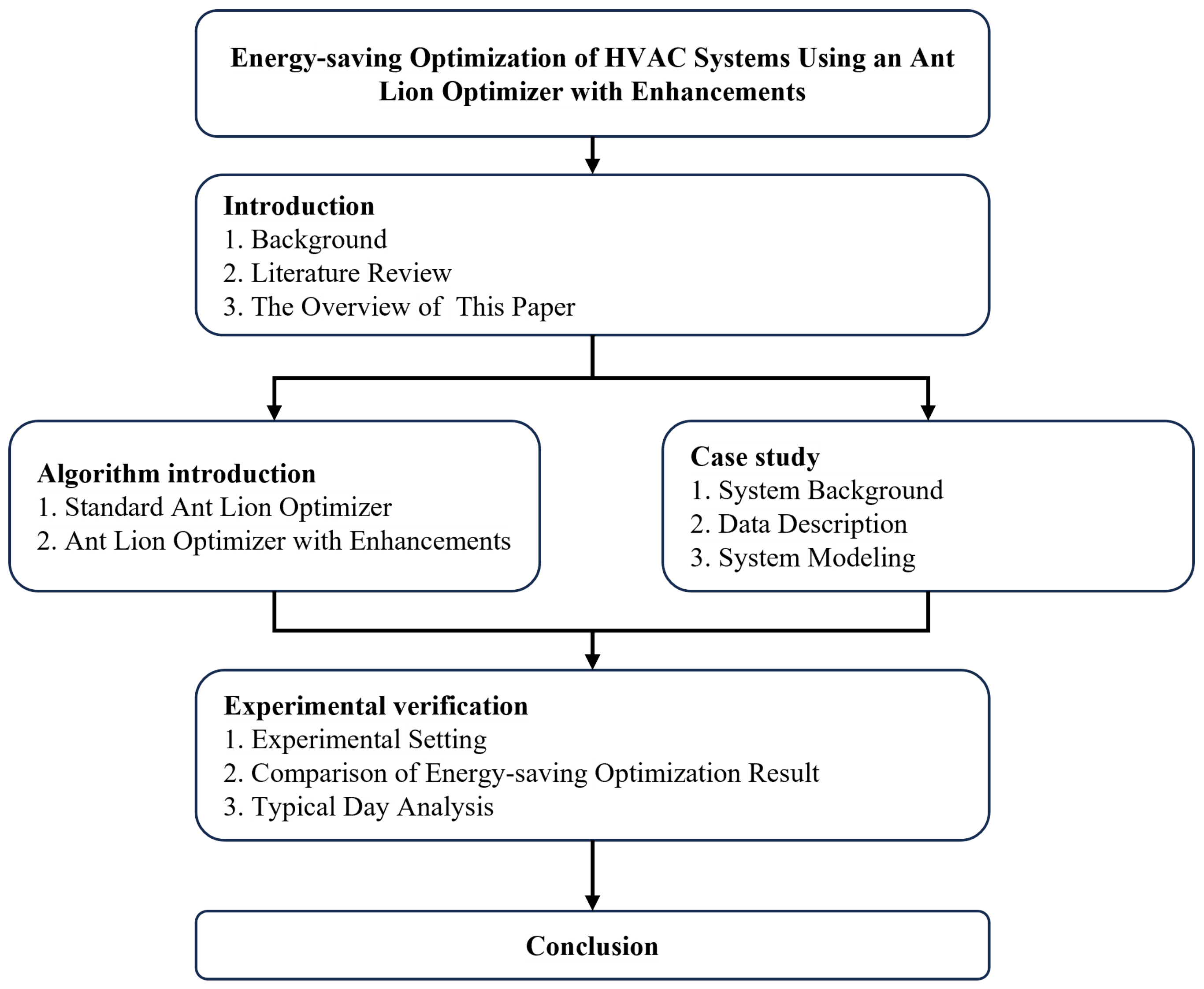
1.3. The Overview of This Paper

Although scholars at home and abroad have made many outstanding contributions in the field of energy-saving optimization of HVAC systems, there are still some challenges. These challenges include the high complexity and specialized knowledge required for physical models, the heavy data dependency, and the limited applicability of data-driven models. Moreover, the control optimization of HVAC systems is prone to local optima due to the high coupling and significant variations in solution space distribution. Existing methods either optimize specific equipment and parameters to achieve local optimal or increase algorithm complexity to trade time for accuracy. Additionally, these methods often experiment under specific conditions, overlooking the distinct characteristics of HVAC systems under various load conditions such as high, medium, and low loads. In response to these issues, this paper makes the following contributions:

(1) To address the complexity and data dependency of current modeling methods of the HVAC system, based on the general mechanism model, this paper utilizes prior knowledge to guide the identification of model parameters. While reducing model complexity and data dependency, it expands the application scope of the model.

(2) To reflect the operational state of the system more accurately, this paper takes into account multiple dimensions in the optimization variables, such as equipment operational status, outlet temperatures, and temperature differences on the chilled and cooling sides, resulting in optimization outcomes that better approximate the optimal operational state of the system.

(3) To balance speed and accuracy in optimization algorithms, this paper proposes an Ant Lion Optimizer with Enhancements (ALOE) that can dynamically adjust the number of populations and the movement trend to improve the convergence speed and optimization ability and randomly adjust the movement amplitude to enhance the local optimal escape ability, which results in fast convergence, stable search efficiency, and superior global optimization capability.

(4) To verify the effectiveness of the proposed method, it was tested under various conditions in a typical office building, achieving energy-saving rates of 28.16%, 28.26%, and 24.9% under high, medium, and low loads, respectively, which are superior to those of other methods.

The structure of the full text is shown in Figure 1.

2. Methodology

Due to the diverse equipment, complex parameters, and strong coupling in HVAC systems, traditional approaches are incapable of comprehensively addressing the entire system or confined to optimizing specific equipment or parameters. While swarm intelligence optimization algorithms employ population-based bio-inspired techniques to effectively handle the coupling problems within systems, they frequently achieve global optimization by augmenting algorithm complexity, sacrificing time for accuracy, thus making their widespread application in practical scenarios challenging. The Ant Lion Optimizer, renowned for its high solution accuracy, minimal parameter adjustment, and ease of implementation, has been extensively applied in scientific research. On this basis, this paper proposes an Ant Lion Optimizer with Enhancements (ALOE) that integrates Levy flight, adaptive elite guidance, and Cauchy mutation to accomplish effective energy-saving optimization for HVAC systems.

2.1. Standard Ant Lion Optimizer

Seyedali Mirjalili proposed the Ant Lion Optimizer (ALO) [17] by studying the bionic mechanism of antlions preying on ants. By modeling the predatory behavior between ants and antlions, antlions are regarded as solutions to the optimization problem. By hunting high-fitness ants, the near-optimal solutions are updated and preserved. The introduction of random walks of ants ensures global search, while the use of roulette wheel selection and elite strategies guarantees population diversity and the optimization performance of the algorithm. Due to its few tuning parameters and high solution accuracy, the ALO algorithm is highly favored by researchers and has been widely applied in engineering fields [27].

The derivation formulas used in this section are derived from reference [17], and the steps of the standard Ant Lion Optimizer algorithm are as follows:

(1)

Initialize Population

Initialize the number of ants N and the dimension D, and randomly initialize the positions of the ants within the search space. Let $X_i$ be the position of ant i, and U and L be the upper and lower boundaries of the search space, respectively. The initial positions of the ants can be expressed by Equation (1).

$$X_i=L+rand(U-L)$$

(1)

The position information is stored in the matrix $M_{Ant}$, which records the positions of the ants. The fitness of the ants, calculated based on the objective function, is stored in $M_{OA}$. The positions of the antlions are also initialized randomly in the same manner and stored in $M_{Antlion}$, with their fitness values saved in $M_{OAL}$. The antlion with the highest fitness is selected as the elite antlion $R_e$, and its position is saved.

(2)

Random Walk

For each ant in $M_{Ant}$, a roulette wheel selection is used to choose an antlion from $M_{Antlion}$. The selected ant then performs a random walk around both the chosen antlion and the elite antlion.

$$X\left(t\right)=\left[0,\mathrm{cumsum}(2r\left(t_1\right)-1),\dots ,\mathrm{cumsum}(2r\left(t_n\right)-1)\right]$$

(2)

Define $X\left(t\right)$ as the position of the ant during the random walk, $consum$ as the cumulative sum, and t as the current iteration number. To ensure that the walking range always remains within the feasible domain, normalize the random walk of the ant.

$$X_i^t={\displaystyle \frac{\left(X_i^t-a_i\right)·\left(d_i^t-c_i^t\right)}{\left(b_i-a_i\right)}}+c_i·t$$

(3)

Let $a_i$ and $b_i$ be the minimum and maximum values of the i-th dimension of the variable during the random walk of the ant X, and $c_i^t$ and $d_i^t$ be the minimum and maximum values of the i-th dimension variable at the t-th iteration. By averaging the random walks around the ordinary antlion $R_a^t$ and the elite antlion $R_e^t$, we ensure that the random walk is always directed towards the global optimum. The position of the ant ${\mathrm{Ant}}_i^t$ is then generated according to Equation (4).

$${\mathrm{Ant}}_i^t={\displaystyle \frac{R_a^t+R_e^t}{2}}$$

(4)

(3)

Hunting Behavior

The random walk of the ants is influenced by the antlion traps, which is simulated by Equation (5).

$$\begin{array}{cc}\hfill c_i^t& ={\mathrm{Antlion}}_j^t+c^t\hfill \\ \hfill d_i^t& ={\mathrm{Antlion}}_j^t+d^t\hfill \end{array}$$

(5)

where $c^t$ is the minimum value of all variables at the t-th iteration, $d^t$ is the vector containing the maximum values of all variables at the t-th iteration, $c_i^t$ is the minimum value of all variables for the i-th ant, and $d_i^t$ is the maximum value of all variables for the i-th ant. The position of the selected j-th antlion at the t-th iteration is denoted as ${\mathrm{Antlion}}_j^t$. This indicates that the ant performs a random walk within a hypersphere defined by the vectors c and d, which surround a selected antlion.

Antlions construct traps to prey on ants, and when ants are in the trap, they continuously slide towards the center of the hypersphere. This behavior can be simulated by Equation (6).

$$\begin{array}{cc}\hfill c^t& ={\displaystyle \frac{c^t}{I}}\hfill \\ \hfill d^t& ={\displaystyle \frac{d^t}{I}}\hfill \end{array}$$

(6)

where I is a ratio, and w is a constant defined based on the current iteration. Specifically, as shown in Equation (7), when $t>0.1T$, $w=2$. When $t>0.5T$, $w=3$. when $t>0.75T$, $w=4$. When $t>0.9T$, $w=5$. And when $t>0.95T$, $w=6$. By adjusting the constant w, the precision level of the exploration can be controlled.

$$I=\left\{\begin{array}{c}1,t\le 0.1T\hfill \\ 1+{10}^w{\displaystyle \frac{t}{T}},t>0.1T\hfill \end{array}\right.$$

(7)

The final step in the predation behavior is when the antlion drags the ant into the sand and devours it. In the algorithm, it is assumed that predation only occurs if the fitness of the ant is higher than the antlion. In this case, the antlion updates its position to the latest position of the preyed ant, as shown in Equation (8).

$${\mathrm{Antlion}}_j^t={\mathrm{Ant}}_i^t\mathrm{if}f\left({\mathrm{Ant}}_i^t\right)>f\left({\mathrm{Antlion}}_j^t\right)$$

(8)

The random walk of the ant population around the elite antlion ensures the convergence of the optimization process, and the roulette wheel operation enhances the global search capability of the ant population to some extent. However, the existing algorithm still has some issues. Firstly, the randomness of the random walk is not strong enough, and uniform walking is not conducive to escaping local optima. Secondly, the proportion of walking around ordinary antlions and elite antlions remains unchanged throughout the optimization process, making it difficult for the algorithm to balance global exploration and local exploitation. Additionally, the algorithm lacks individual mutation strategies, which limits population diversity and weakens the global search capability.

2.2. Ant Lion Optimizer with Enhancements

The standard ALO algorithm has a restricted ability to escape local optima and cannot dynamically adjust exploration and exploitation. To resolve these issues, this paper introduces the Levy flight mechanism, the adaptive elite guidance mechanism, and the dynamic Cauchy mutation mechanism to boost the performance of the algorithm. Levy flight [28], with its frequent short-distance movements and occasional long-distance movements, enhances the ability of the algorithm to escape local optima. The adaptive elite guidance mechanism dynamically adjusts the importance of the walking strategy according to different stages of the optimization process, improving the exploration capability of the algorithm in the early stages and exploitation capability in the later stages. The dynamic Cauchy mutation mechanism selects antlions with poorer fitness for Cauchy mutation [29] based on the proportional coefficient $\beta$, increasing population diversity and enhancing the optimization capability of the algorithm.

2.2.1. The Levy Flight of the Ant Mechanism

Levy flight is a random strategy that includes frequent short-distance walks and occasional long-distance walks. This strategy ensures detailed exploration of the nearby region by the population while introducing a degree of mutation. The alternation of these two methods enables thorough traversal of the solution space, thereby enhancing the global search capability of the algorithm. Levy flight follows the Levy distribution, with its probability density function given by Equation (9).

$$P_{\alpha ,\gamma }\left(z\right)={\displaystyle \frac{1}{\pi }}·{\int }_0^{\infty }exp\left(-\gamma q^{\alpha }\right)cos\left(qz\right)dq$$

(9)

Typically, random numbers following the Levy distribution are generated using simulation methods for analysis. To ensure that the Levy flight trajectory thoroughly traverses the designated solution space, the simulation formula [30] has been modified as Equation (10).

$$\left\{\begin{array}{c}{{\delta }_{\mu }=\left\{{\displaystyle \frac{\Gamma \left(1+\beta \right)·sin\left(\pi ·\beta /2\right)}{\Gamma \left[\left(1+\beta \right)/2\right]2^{\left(\beta -1\right)/2}·\beta }}\right\}}^{1/\beta }\hfill \\ {\delta }_v=1\hfill \end{array}\right.$$

(10)

$$\left\{\begin{array}{c}\mu \sim N\left(0,{\delta }_{\mu }^2\right)\\ v\sim N\left(0,{\delta }_v^2\right)\end{array}\right.$$

(11)

$$\left\{\begin{array}{c}{\displaystyle S=\frac{\mu }{{\left|v\right|}^{1/\beta }}}\hfill \\ {\lambda }_i=cumsum\left(S_i\right)\hfill \end{array}\right.$$

(12)

In the formula, $i=1,2,\cdots ,n$ represents the optimization dimensions, and $cumsum\left(S_i\right)$ is the cumulative sum of the positions from the first i Levy flights.

$$L\left({\lambda }_i\right)=\left\{\begin{array}{cc}{l}_b,\hfill & {\lambda }_i<l_b\\ a·{\lambda }_i,\hfill & l_b<{\lambda }_i<u_b\\ u_b,\hfill & {\lambda }_i>u_b\end{array}\right.$$

(13)

The Levy flight trajectory is calculated using Equations (10)–(12). Equation (13) maps the Levy flight position into the solution domain $\left[l_b,u_b\right]$ using the scaling factor a and a limiting operation.

2.2.2. The Adaptive Elite Guidance Mechanism

The standard antlion algorithm uses Equation (4) to calculate the average of the two random walks, $R_a^t$ and $R_e^t$, to balance exploration and exploitation capabilities. However, it overlooks that the proportion of exploration and exploitation should vary at different stages. This paper improves the proportional coefficients of $R_a^t$ and $R_e^t$, allowing the weights of the two walking strategies to differ at various stages. In the early stages, the algorithm primarily focuses on walking around the antlions selected by the roulette wheel, enhancing global exploration. In the later stages, it emphasizes walking around the elite antlion to increase convergence speed. The improved dynamic proportional coefficients are shown in Equation (14).

$$An{t}_i^t=cos\left({\displaystyle \frac{t}{2·T}}·\pi \right)·R_a^t+sin\left({\displaystyle \frac{t}{2·T}}·\pi \right)·R_e^t$$

(14)

$R_a^t$ represents the position of the ant after performing a random walk around the antlion selected by the roulette wheel at iteration t, and $R_e^t$ represents the position of the ant after performing a random walk around the elite antlion at iteration t. T is the maximum number of iterations, and t is the current iteration number. With the improvements in Equation (14), the algorithm initially focuses on walking around the ordinary antlions selected by the roulette wheel to ensure the global exploration capability of the entire solution space, while gradually increasing the weight of the optimal antlion to ensure the direction of optimization. In the later stages, the algorithm primarily focuses on walking around the elite antlion to quickly converge towards the global optimum position and utilizes a lower proportion of walks around ordinary antlions to introduce some randomness. This effectively improves the exploration capability in the early stages and the exploitation capability in the later stages. Additionally, the use of dynamic proportional coefficients also enhances the diversity of the ant population to some extent.

2.2.3. Dynamic Cauchy Variation Mechanism

As shown in Equation (6), an antlion can only update to a higher fitness position if it preys on an ant with a higher fitness than itself. If there are no ants with higher fitness within its trap range, the antlion tends to be stuck in a local optimum. In such cases, the antlion will struggle to prey on ants from its original position, weakening the diversity and optimization capability of the population. Therefore, mutation operations are necessary for such antlions. The Cauchy mutation operator [31] can significantly enhance the global exploration ability, the convergence precision, and the stability of the algorithm. The Cauchy distribution is shown in Equation (15).

$$f(x;x_0,\gamma )={\displaystyle \frac{1}{\pi ·\gamma ·\left[1+{\left(\frac{x-x_0}{\gamma }\right)}^2\right]}}={\displaystyle \frac{1}{\pi }}·\left[{\displaystyle \frac{\gamma }{{(x-x_0)}^2+{\gamma }^2}}\right]$$

(15)

Therefore, this paper proposes a dynamic Cauchy mutation strategy based on the Cauchy mutation operator. The mutation process is shown in Equation (16). In the equation, $X^{\prime }$ represents the updated position of the initial position X, $\mathrm{Cauchy}(0,1)$ is the standard Cauchy random distribution at $t=1$, the parameter $\eta$ is a constant used to control the mutation intensity of the Cauchy distribution.

$$X^{\prime }=X+\eta ·\mathrm{Cauchy}(0,1)$$

(16)

This strategy sorts the N antlions by fitness and selects the S antlions with poorer fitness according to the proportion $\beta$ as shown in Equation (17).

$$S=\beta ·N$$

(17)

Since the number of mutated individuals affects the performance of the algorithm differently at various optimization stages, the proportional coefficient $\beta$ is dynamically adjusted through Equation (18) at different stages of the optimization process.

$$\beta =0.5-{\left({\displaystyle \frac{t}{2·T}}\right)}^2$$

(18)

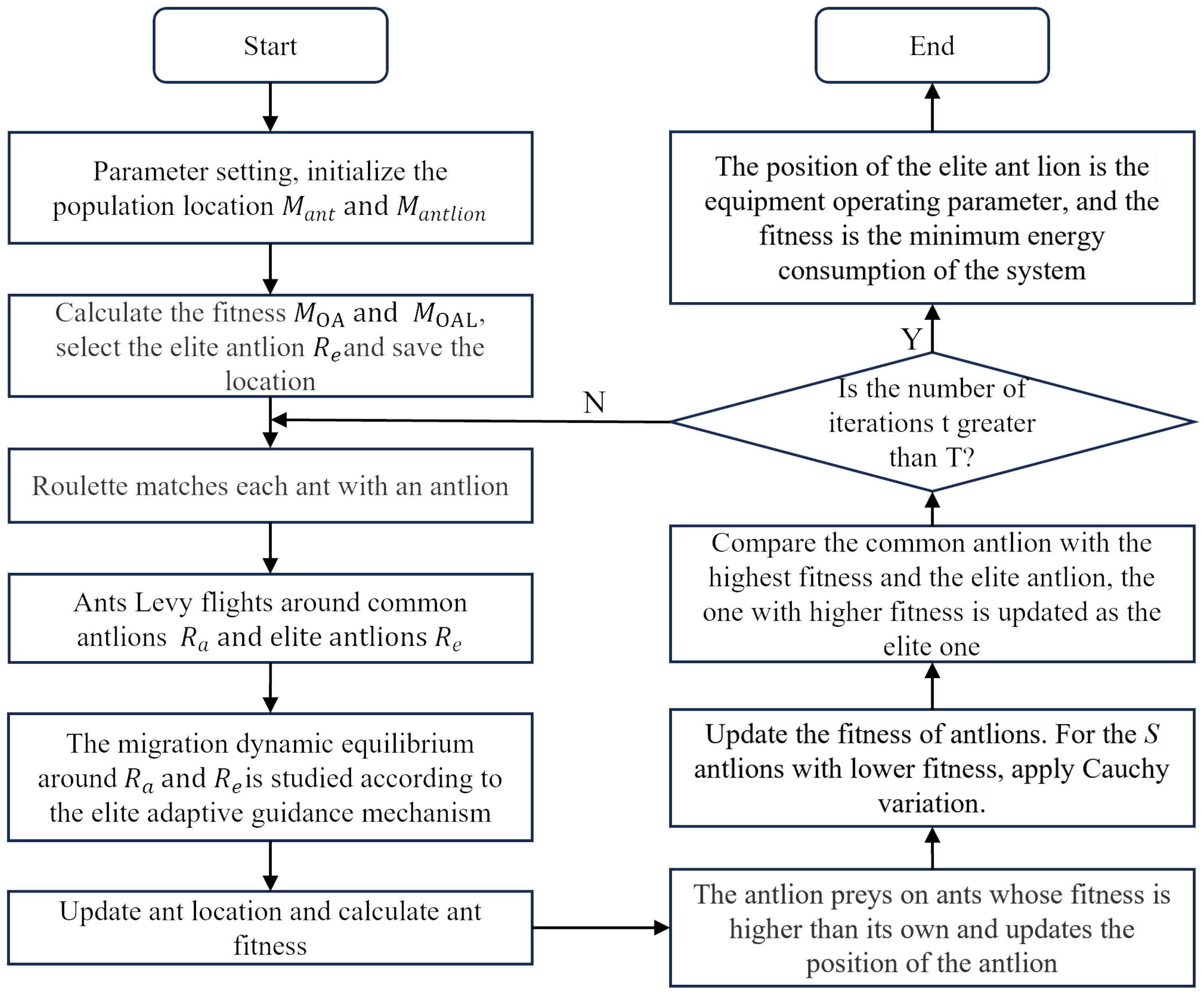
2.2.4. Algorithm Flow

In the actual HVAC system, optimizing for minimal energy consumption is a multi-extremum optimization problem. Due to significant differences and coupling between the characteristics of various devices, multiple local minima can easily occur, and solutions within the search space are highly unevenly distributed. The standard antlion algorithm is hard to apply to this optimization problem due to its poor ability to escape local optima and inability to dynamically adjust parameters. Therefore, this paper proposes the ALOE algorithm. In ALOE, Levy flight uses frequent short-distance and occasional long-distance walks to balance the local exploitation and global exploration capabilities of the algorithm, enhancing the ability to escape local optima. The adaptive elite guidance mechanism adjusts the weights of walking around elite and ordinary antlions at different optimization stages to improve the exploration capability of the algorithm in the early stages and exploitation capability in the later stages, enhancing convergence speed and global optimization capability. The dynamic Cauchy mutation mechanism selects S antlions with poorer fitness for Cauchy mutation according to a dynamic proportion $\beta$ at different optimization stages, ensuring the diversity and convergence speed of the antlion population.

The basic steps of the ALOE algorithm are summarized as follows:

(a)

Initialize the positions of the ant and antlion populations, $M_{ant}$ and $M_{antlion}$.

(b)

Calculate the fitness of the ants and antlions, $M_{OA}$ and $M_{OAL}$, select the elite antlion $R_e$, and save its position.

(c)

Use the roulette wheel to select the antlion $R_a$ around which each ant will walk.

(d)

The ants perform Levy flights around $R_e$ and $R_a$.

(e)

Dynamically balance the walks around $R_e$ and $R_a$ according to the adaptive elite strategy.

(f)

Update the positions of the ants $M_{ant}$ and calculate their fitness $M_{OA}$.

(g)

The ants fall into traps, and the antlions prey on the ants, updating their positions $M_{antlion}$ according to Equation (8).

(h)

Update the fitness of the antlions and apply the Cauchy mutation to the $\beta ·N$ antlions with the lowest fitness.

(i)

Compare the fitness of the best antlion with the elite antlion, and if the former is better, update the elite antlion $R_e$.

Repeat steps (c)–(i) until the maximum number of iterations is reached. The flowchart of the improved enhanced antlion optimization algorithm is shown in Figure 2.

3. Case Study

An accurate system energy consumption model plays a crucial role in the energy-saving optimization of HVAC systems. However, this system consists of numerous devices that have strong coupling among them and involve significant heat exchange and energy conversion processes during operation. Therefore, in this section, the principle of the system is analyzed. First, individual devices are modeled based on the universal mechanism model, and parameter identification is carried out according to historical data. Then, they are integrated into the entire system according to the system topology. This enables the HVAC system model to describe the system state more accurately, including flow rate, energy consumption, and heat.

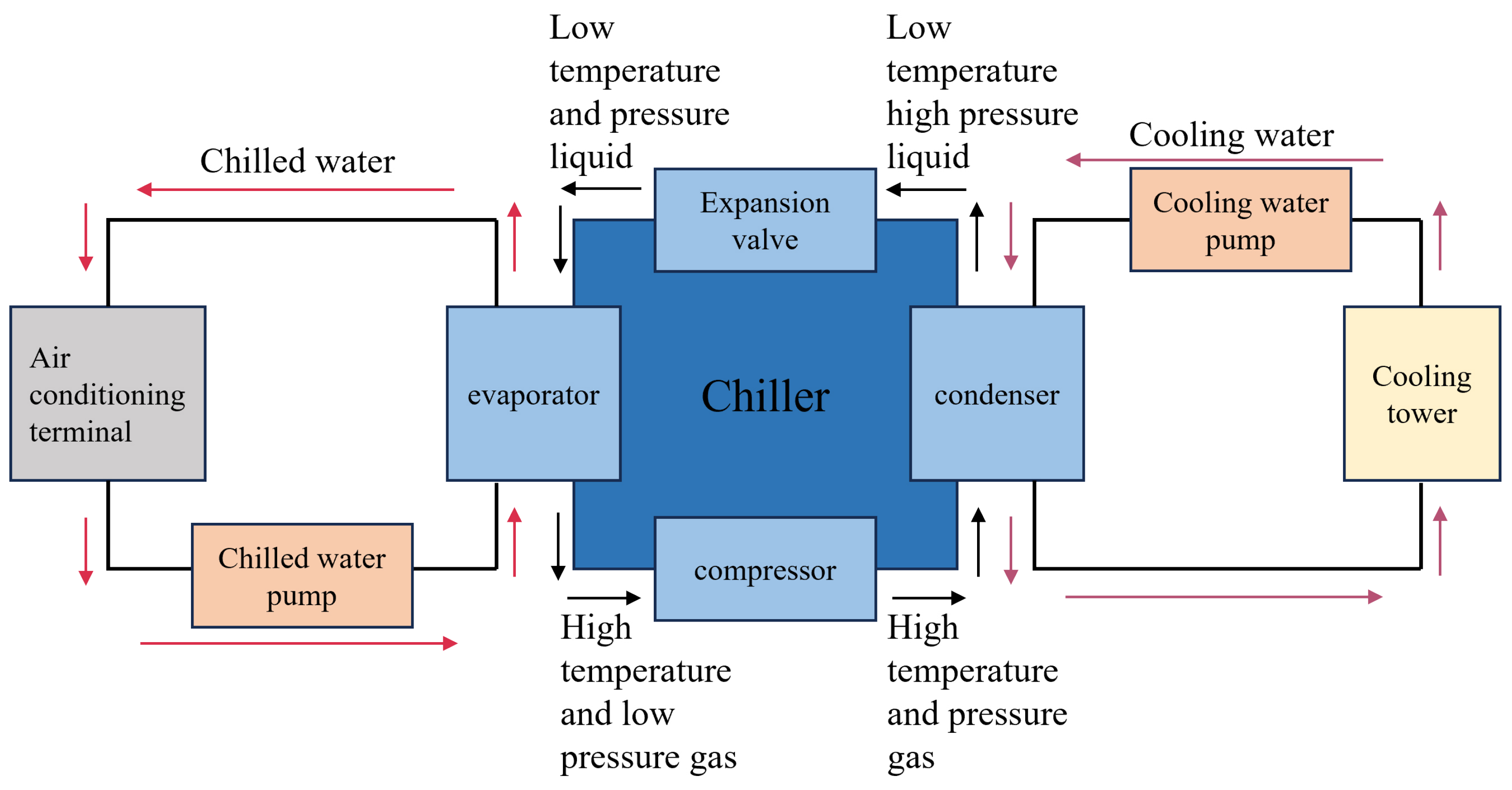
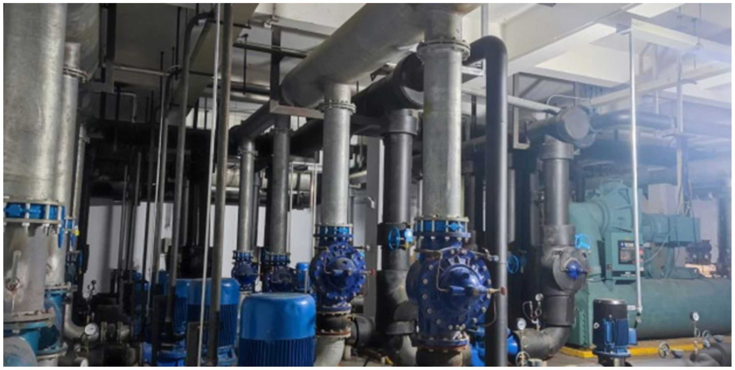
3.1. System Background

The HVAC system is the primary energy-consuming part of a building, and understanding the operating principles is crucial for improving building energy efficiency. The system typically consists of chillers, chilled water pumps, cooling water pumps, and cooling towers. These components form three interrelated cycles that couple together to create the HVAC system: the chilled water cycle, the refrigerant cycle, and the cooling water cycle. The operating parameters of each cycle influence and connect. The operating principle diagram of the system is shown in Figure 3.

High-temperature chilled water releases heat in the evaporator of the chiller, converting it into low-temperature chilled water. This low-temperature water is then driven by a pump to the fan coil units situated in designated areas of the building, where it takes part in heat exchange at the terminal end of the indoor air conditioning system, absorbing heat and reducing the surrounding temperature. The heated high-temperature chilled water then cycles back to the chiller, completing the chilled water cycle. The cooling water cycle handles the heat exchange between the chiller and the outdoors; low-temperature cooling water absorbs heat in the condenser of the chiller, and is then pumped to an outdoor cooling tower by the cooling water pump, and releases the heat outdoors through the cooling tower. The cooled water flows back to the condenser of the chiller for the next cooling water cycle.

3.2. Data Description

The case study for this research is an office building in a technology park located in the Binjiang District of Hangzhou. The total construction area is approximately 32,000 square meters, with an above-ground area of 30,069.1 square meters and an underground area of 1912.95 square meters. The main buildings of the technology park are divided into Area A, Area B, Area C, Area D, the glass hall, and the underground parking garage. Areas A, B, C, and D primarily consist of factory buildings and office buildings, while the glass hall is mainly used for exhibitions. There is also a one-story underground parking garage. The aerial view of the entire building is shown in Figure 4.

The entire building is cooled using an HVAC system, with the chiller located in the basement of Building A. After being cooled, the chilled water is distributed to each floor of Buildings A, B, C, and D through a water distributor. The system has been in use for many years. The topology of the HVAC system and the field equipment are shown in Figure 5 and Figure 6, respectively.

The parameters and quantities of the HVAC system equipment are listed in

Table 2. Device parameters of cooling system.

Equipment Type	Parameters	Quantity
Chiller1	Rated cooling capacity 1934 kW, rated power 336 kw	1
Chiller2	Rated cooling capacity 1135 kW, rated power 261 kw	1
Chiller3	Rated cooling capacity 353.5 kW, rated power 74 kw	1
Chilled water pump	Rated flow 80 m3/h, rated power 15 kw	1
Chilled water pump	Rated flow 200 m3/h, rated power 30 kw	2
Chilled water pump	Rated flow 400 m3/h, rated power 55 kw	2
Cooling water pump	Rated flow 250 m3/h, rated power 30 kw	2
Cooling water pump	Rated flow 450 m3/h, rated power 45 kw	2
Cooling Tower	Rated flow 250 m3/h, rated power 7.5 kw	4

. Data were collected from 1 April 2023 to 31 October 2023, with a sampling interval of 5 min, resulting in a total of 61,632 observations. This dataset includes information on the status of all equipment (chillers, water pumps, cooling towers), outdoor temperature, outdoor relative humidity, cooling water outlet temperature, cooling water temperature difference and flow rate, chilled water outlet temperature, chilled water temperature difference, and flow rate. The cooling load of the building is calculated based on the last three variables. The original data collected need to be cleaned, the missing values are processed first, and the missing data at different time points are filled forward or backward. Secondly, outlier processing is carried out. According to the cause of abnormal data, unit transformation, tail reduction, or curve fitting are used to deal with it.

3.3. System Modeling

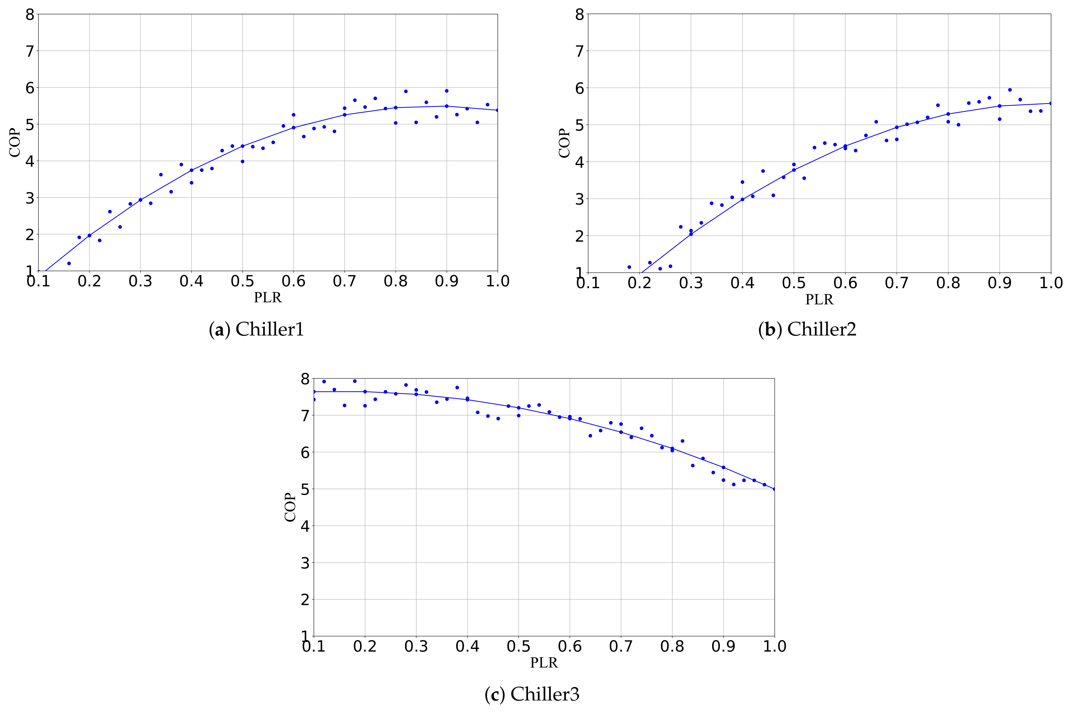
3.3.1. Model for Chiller

For the simulation of chillers, it is necessary to establish an accurate mathematical model to reflect the relationships between various parameters. Generally, the study focuses on the chilled water flow rate, chilled water outlet temperature, return water temperature under multiple conditions, as well as the cooling capacity and COP of the chiller under fluctuating loads. The cooling capacity of the chiller under different operating conditions can be expressed by Equation (19).

$$\mathrm{COP}={\mathrm{a}}_1+{\mathrm{b}}_1·\left(\mathrm{PLR}\right)+{\mathrm{c}}_1·{\left(\mathrm{PLR}\right)}^2$$

(19)

$a_1$, $b_1$, and $c_1$ are the polynomial coefficients, and $PLR$ represents the part load ratio of the chiller. The derivation of COP and PLR is derived from [32], the calculation method for the total load capacity $Q_{\mathrm{met}}$ (J) of the chiller is shown in Equation (20).

$${\mathrm{Q}}_{\mathrm{met}}={\mathrm{m}}_{\mathrm{chw}}·{\mathrm{Cp}}_{\mathrm{chw}}·\left({\mathrm{T}}_{\mathrm{chw},\mathrm{in}}-{\mathrm{T}}_{\mathrm{chw},\mathrm{out}}\right)$$

(20)

$Tchw,out$ (°C) represents the outlet temperature of the chilled water pump, ${Cp}_{\mathrm{chw}}$ (J/(kg · °C) represents the specific heat capacity of the fluid entering the chilled water pump, $m_{\mathrm{chw}}$ (kg) represents the flow rate of chilled water in the chiller.

$$Q_{\mathrm{rejected}}=m_{cw}·C{p}_{cw}·\left(T_{cw,\mathrm{in}}-T_{cw,\mathrm{out}}\right)$$

(21)

$T\mathrm{cw},\mathrm{out}$ represents the outlet temperature of the cooling water pump, ${\mathrm{Cp}}_{\mathrm{cw}}$ represents the specific heat capacity of the fluid entering the cooling water pump, and $m_{\mathrm{cw}}$ represents the flow rate of cooling water in the chiller. $Q_{\mathrm{rejected}}$ represents the energy released by the chiller to the surrounding environment, from which the actual power of the chiller can be derived by Equation (22).

$$P=Q_{\mathrm{rejected}}-Q_{\mathrm{met}}$$

(22)

P represents the actual power consumed by the chiller, the COP can be expressed by Equation (23).

$$\mathrm{COP}={\displaystyle \frac{Q_{\mathrm{met}}}{P}}$$

(23)

$Q_{\mathrm{load}}$ represents the load of the chiller, and the calculation method for $Q_{\mathrm{load}}$ is as Equation (24).

$$Q_{\mathrm{load}}=m_{\mathrm{chw}}·{\mathrm{Cp}}_{\mathrm{chw}}·(T_{\mathrm{chw},\mathrm{in}}-T_{\mathrm{chw},\mathrm{set}})$$

(24)

$m_{\mathrm{chw}}$ represents the flow rate of chilled water entering the chiller, $T_{\mathrm{chw},\mathrm{in}}$ represents the inlet temperature of the chilled water pump, $T_{\mathrm{chw},\mathrm{set}}$ represents the set temperature of the chilled water pump, ${Cp}_{\mathrm{chw}}$ represents the specific heat capacity of the fluid entering the chilled water pump, Capacity represents the chiller capacity under current conditions. The part load ratio at this time can be expressed by the following Equation (25).

$$\mathrm{PLR}={\displaystyle \frac{Q_{\mathrm{load}}}{\mathrm{Capacity}}}$$

(25)

The coefficients can be obtained through data fitting, with specific coefficients corresponding to each operating condition. Based on this, a more accurate model can be further refined. Under the conditions where the chilled water outlet temperature is 7 °C, and the cooling water outlet temperature is 30 °C, the COP curve fitted by the model in this paper is compared with the actual COP, as shown in Figure 7.

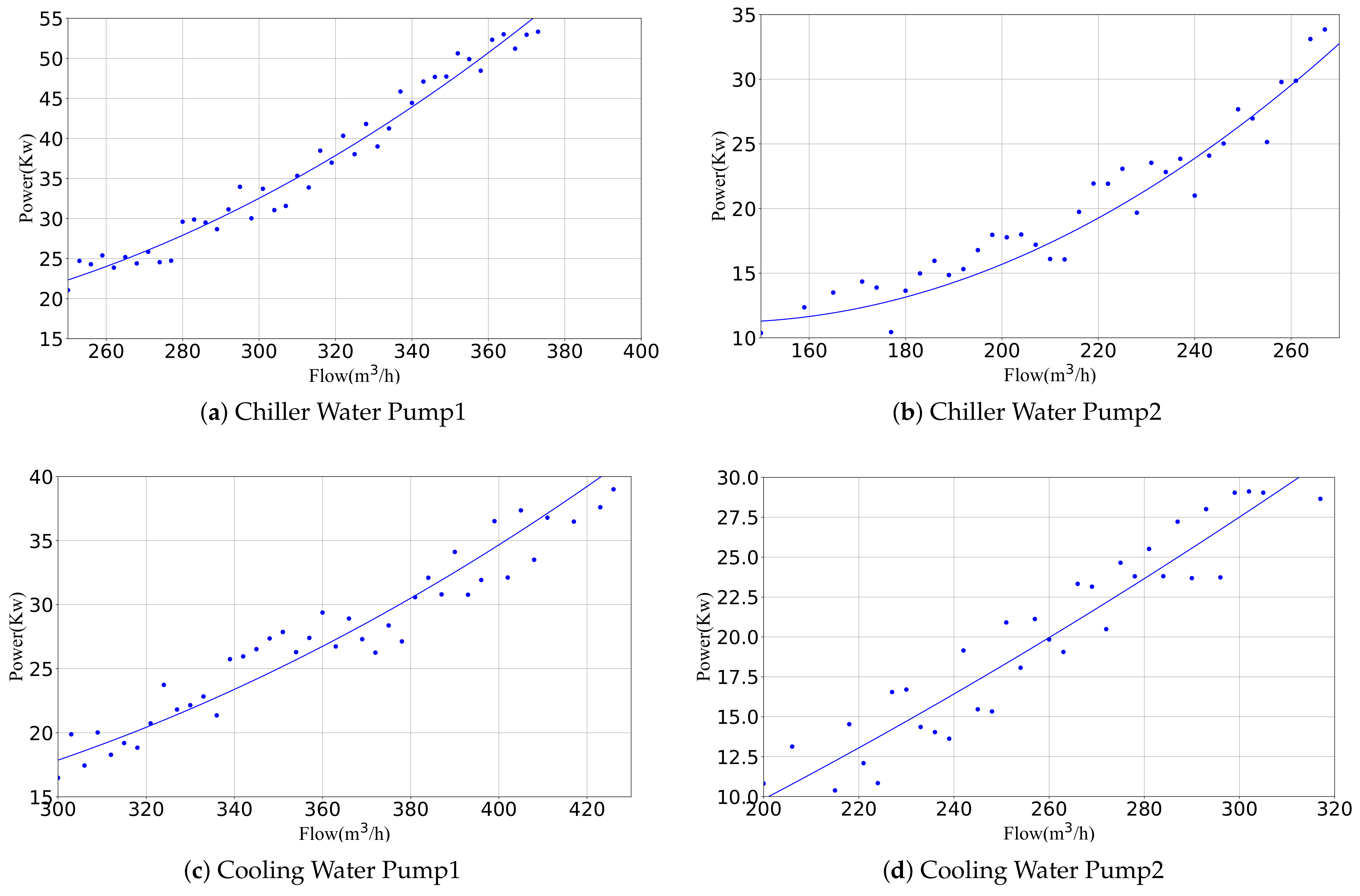
3.3.2. Model for Cooling/Chilled Water Pump

The variable frequency pump contains the refrigeration pump and the cooling pump, the main power equipment in the chilled water cycle and the cooling water cycle, and plays the role of transporting water. First, according to Equation (26), determine whether the target set flow rate Q (m³/h) is less than the upper limit flow rate $Q_m$.

$$Q_{\mathrm{m}}=Q_0·{\displaystyle \frac{f_{\mathrm{m}}}{50}}$$

(26)

If the flow rate surpasses the limit, it is computed according to the maximum frequency. Otherwise, it is computed based on the variable frequency operation of the pump. Based on formula derivation in reference [33], the relationship between flow rate (m³/h), frequency (Hz), and power (kW) is shown in Equation (27).

$$\left\{\begin{array}{c}{\displaystyle \frac{Q}{Q_0}}={\displaystyle \frac{f}{f_0}}\hfill \\ {\displaystyle \frac{H}{H_0}}={\left({\displaystyle \frac{f}{f_0}}\right)}^2\hfill \\ {\displaystyle \frac{\mathrm{P}}{{\mathrm{P}}_0}}={\left({\displaystyle \frac{\mathrm{f}}{{\mathrm{f}}_0}}\right)}^3\hfill \end{array}\right.$$

(27)

The frequency ratio of the pump, which is the pump speed ratio, is denoted as n. Combining this with Equation (27), the flow rate-head curve of the variable frequency pump is shown in Equation (28).

$$H=a·Q^2+b·Q_{0}n+c·n^2$$

(28)

Additionally, considering the impedance from the chiller and pump, as well as the impedance of the chiller pipelines and terminal pipelines, the pipeline impedance in the system is given by Equation (29).

$$S_a=S_c+S_d+S_e$$

(29)

By substituting the set flow rate into the pipeline characteristic curve equation, the head at the current operating point of the variable frequency pump can be calculated as Equation (30).

$$H=S_a·Q^2$$

(30)

Then, combined with the variable frequency pump Equation (28), the current pump speed ratio is shown in Equation (31).

$$\mathrm{c}·{\mathrm{n}}^2+\mathrm{b}·{\mathrm{Q}}_0·\mathrm{n}+\mathrm{a}·{\mathrm{Q}}^2-\mathrm{H}=0\Rightarrow \mathrm{n}={\displaystyle \frac{-\mathrm{b}·{\mathrm{Q}}_0+\sqrt{{\mathrm{b}}^2·{\mathrm{Q}}_0^2-4·c\left(\mathrm{a}·{\mathrm{Q}}^2-\mathrm{H}\right)}}{2·c}}$$

(31)

Finally, substitute the speed ratio into Equation (27) to calculate the energy consumption of the pump.

$$P=P_0·n^3$$

(32)

For the four kinds of variable frequency pumps used in this case, the pump characteristic curves fitted by the model in this section are shown in Figure 8.

3.3.3. Model for Cooling Tower

The cooling tower uses water as the circulating coolant, absorbing heat from the cooling water and releasing it into the atmosphere through heat exchange with air and spray water. Based on the enthalpy values of moist air at the inlet and outlet of the cooling tower, $h_{a,o}$ (J/kg) and $h_{a,i}$, the heat dissipation of the cooling tower can be calculated as Equation (33).

$$Q=\epsilon m_a(h_{a,o}-h_{a,i})$$

(33)

In Equation (33), $\epsilon$ represents the heat exchange efficiency of the cooling tower, and $m_a$ is the mass of dry air entering the heat exchange. The enthalpy of moist air, based on the wet-bulb temperature t, is fitted using the Equation (34).

$$h=a+b·t+c·t^2$$

(34)

By querying the number of heat transfer units $NTU$ and the heat capacity ratio of air to water n in equipment parameters, and the mechanism model derivation formula of cooling tower module in trnsys software, the heat exchange efficiency $\epsilon$ can be calculated according to Equation (35).

$$\epsilon ={\displaystyle \frac{1}{n}}\left(1-exp\left(-n(1-exp(-NTU\left)\right)\right)\right)$$

(35)

Therefore, the cooling tower outlet water temperature $T_{w,out}$ can be calculated based on the inlet water flow rate $m_{i}n$ and the inlet water temperature $T_{in}$ can be calculated as Equation (36).

$$T_{w,out}=T_{in}-{\displaystyle \frac{Q}{c{m}_{in}}}$$

(36)

In Equation (36), c is the specific heat capacity of water. For a fixed-frequency cooling tower, the current power $P\left(kW\right)$ is primarily determined by the rated power of the fan $P_{rated}\left(kW\right)$ and the number of fans in operation N, as Equation (37).

$$P=N·P_{rated}$$

(37)

When the outlet water temperature of the cooling tower is lower than the set value for some time, the fans of the cooling tower are turned off. Conversely, when the outlet water temperature exceeds the set value for some time, if the fans are in the off state, the fans are turned on. If all the fans have been completely opened and the water temperature still cannot reach the set value, the user will receive notifications that the set water temperature cannot be achieved.

3.3.4. System Energy Consumption Model

Based on the models of the system equipment discussed earlier, the energy consumption model of the entire system can be established, as shown in Equation (38).

$$\begin{array}{cc}\hfill & F_{\mathrm{obj}}=P_{\mathrm{system}}\hfill \\ \hfill & =P_{\mathrm{chiller}}+P_{\mathrm{chilled\_water\_pump}}+P_{\mathrm{cooling\_water\_pump}}+P_{\mathrm{cooling\_tower}}\hfill \\ \hfill & =F(Q_{\mathrm{load}},t,\mathrm{hu},\mathrm{state},t_{w,\mathrm{e},\mathrm{L}},\delta t_{w,\mathrm{e},\mathrm{L}},t_{w,\mathrm{c},\mathrm{L}},\delta t_{w,\mathrm{c}})\hfill \end{array}$$

(38)

In Equation (38), the cooling load $Q_{Load}$, temperature t, and humidity $hu$ are actual on-site environmental parameters. $statet$ represents equipment status information, $t_{w,\mathrm{e},\mathrm{L}}$ represents the chilled water outlet temperature, $\delta t_{w,\mathrm{e},\mathrm{L}}$ represents the chilled water temperature difference, $t_{w,\mathrm{c},\mathrm{L}}$ represents the cooling water outlet temperature, and $\delta t_{w,\mathrm{c}}$ represents the cooling water temperature difference. Based on $Q_{Load}$, $\delta t_{w,\mathrm{e},\mathrm{L}}$, and $\delta t_{w,\mathrm{c}}$, the flow rates of chilled water and cooling water are determined using Equation (25). Then, the total power of the chiller $P_{\mathrm{chiller}}$ is calculated using Equations (21)–(23). The pump speed ratio is calculated using Equation (32), and the power of the variable frequency pump, which is proportional to the cube of the pump speed ratio, is calculated using Equation (33). The power of the fixed-frequency pumps is determined by their rated power and on/off state. Thus, the total power of the chilled water pump and cooling water pump, $P_{chilled\_water\_pump}$ and $P_{cooling\_water\_pump}$, can be calculated. Similarly, the power of the cooling tower, $P_{cooling\_tower}$, which operates at a fixed frequency, can be directly calculated based on the on/off information in $state$ and its rated power. The goal of this paper is to optimize the energy efficiency of the HVAC system. Therefore, the optimization objective is to minimize the energy consumption $P_{system}$ of the system by searching for the optimal $statet$, $t_{w,e,L}$, $\delta t_{w,e,L}$, $t_{w,c,L}$, and $\delta t_{w,c}$ within the search space.

4. Experiment

4.1. Experimental Setting

4.1.1. Hyperparameters

In swarm intelligence algorithms, the number of individuals and the maximum number of iterations are crucial parameters. To ensure the fairness of the comparison of the energy-saving optimization effect, it is essential to unify the hyperparameter settings of the algorithm. The maximum number of individuals in the population and the number of iterations are set to 50 and 400, respectively. The parameter settings for other comparison optimization algorithms are determined based on their optimal performance. The significant parameter settings for the comparison algorithms involved in this experiment are shown in

Table 3. Key Configuration Parameters of the Algorithm.

Algorithm	Parameter	Function	Value
BRO [19]	threshold	dead threshold	3
DMOA [20]	n_baby_sitter	number of babysitters	3
	peep	define vocalization coeff	2
GSKA [22]	pb	percent of the best	0.1
	kr	knowledge ratio	0.7
HBO [23]	degree	the degree level in corporate rank hierarchy	2
WHO [25]	n_explore_step	number of exploration step	3
	n_exploit_step	number of exploitation step	3
	eta	learning rate the	0.15
		probability of wildebeest
	p_hi	move to another position	0.9
		based on herd instinct
	local_alpha	control local movement	0.9
	local_beta	control local movement	0.3
	global_alpha	control global movement	0.2
	global_beta	control global movement	0.8
	delta_w	dist to worst	2.0
	delta_c	dist to best	2.0

.

4.1.2. Evaluation Metrics

To more accurately verify the effectiveness of the algorithm in HVAC system optimization, this experiment first evaluated the error of the system energy consumption model, and the calculation method was as follows:

$$Error={\displaystyle \frac{|Predicted-Actual|}{Actual}}·100\%$$

(39)

$Predicated$ (kWh) is the system energy consumption calculated by the system energy consumption model based on input cooling load, equipment status, and other information. $Actual$ (kWh) is the actual energy consumption of the system. This metric can prove that the algorithm is optimized on an accurate model.

This experiment evaluates the effect of the algorithm from three aspects: running time, energy-saving effect, and stability [2]. According to the results of multiple experiments under the same conditions. If $T_i$ represents the convergence time of the i-th run, and the total number of runs is N, then the average running time ($ART$) can be expressed as:

$$ART={\displaystyle \frac{1}{N}}\sum _{i=1}^N{T}_i$$

(40)

The energy-saving effect of the algorithm is evaluated by the energy-saving rate ($ESR$), which is calculated as follows:

$$ESR={\displaystyle \frac{E_{old}-E_{new}}{E_{old}}}·100\%$$

(41)

where $E_{old}$ (kWh) is the energy consumption of the HVAC system when it is managed only according to human experience without using an optimization algorithm, $E_{new}$ (kWh) is the operating energy consumption of the system after optimization utilizing the algorithm.

Therefore, the energy-saving rate of the i experiment is denoted as $ES{R}_i$, then the average energy-saving rate $\overline{ESR}$ of multiple experiments is calculated as:

$$\overline{ESR}={\displaystyle \frac{1}{N}}\sum _{i=1}^{N}ES{R}_i$$

(42)

The stability of the algorithm is also evaluated according to the variance of the energy-saving rate ($VESR$) of multiple experiments. The energy-saving rate of the i experiment is $ES{R}_i$, and the expected energy-saving rate of multiple experiments is $\overline{ESR}$, the calculation method is as follows:

$$\mathrm{VESR}={\displaystyle \frac{1}{N}}\sum _{i=1}^N{(ES{R}_i-\overline{ESR})}^2·100\%$$

(43)

4.2. Comparison of Energy-Saving Optimization Results

The data for this experiment are from the day with the highest cooling load in the summer of 2023. The trend of the cooling load variation throughout the day is shown in Figure 9.

When the HVAC system starts at 7 a.m., the cooling load increases and reaches its peak at 3 p.m., then gradually decreases. Based on the distribution characteristics of the cooling load, this experiment selected three representative cooling load states of the day: the period with the highest cooling load (high load scenario), the period with 60% of the peak cooling load (medium load scenario), and the period with 30% of the peak cooling load (low load scenario). Each period is a 30-minute window.

To verify the accuracy of the HVAC system model established in Section 3.3, experiments were carried out under three cooling load scenarios. First, obtain the actual operating status of the device, ambient temperature and humidity information, chilled water outlet temperature, and corresponding cooling load in the three scenarios. The data are input into the simulation model to predict the system energy consumption. As shown in

Table 4. Comparison of actual energy consumption with the energy consumption predicted by the model.

Case	Temperature	Humidity	Result	CHW Pump	CW Pump	Cooling Tower	Chiller	System
High	34.28	35.78	Actual Predicted Error	27.62	20.40	10.28	156.00	214.28
				27.48	22.55	12.97	139.60	201.60
				0.36%	10.39%	16.73%	10.51%	5.92%
Medium	30.53	54.22	Actual Predicted Error	28.77	26.13	4.21	51.75	110.87
				27.74	24.02	4.60	55.64	112.00
				3.60%	8.10%	9.38%	7.51%	1.02%
Low	32.26	43.18	Actual Predicted Error	6.62	10.11	1.78	19.52	38.03
				6.27	9.84	1.74	22.74	40.60
				5.26	2.62	2.32	16.50	6.74
-	-	-	Mean Error	3.07%	7.00%	9.48%	11.51%	4.56%

‘Actual’ indicates the actual energy consumption of the equipment, ‘Predicted’ indicates the energy consumption of the equipment predicted by the simulation model under the same conditions, and ‘Error’ indicates the deviation between the predicted value and the actual value.

, the actual total energy consumption of the system under high, medium, and low loads is 214.28 kWh, 110.87 kWh, and 38.03 kWh, while the total energy consumption predicted by the simulation model is 201.6 kWh, 112.00 kWh and 40.60 kWh, respectively. The errors were 5.92%, 1.02%, and 6.74%, respectively. The average error of the cooling tower and chiller is 9.48% and 11.51%. The reason is that the measurement error of the flowmeter is large, which makes the second-order mathematical model established in Section 3.3 fully fit its characteristic curve. In general, the average error of the total energy consumption is 4.56%, which verifies that the HVAC model established in Section 3.3 has accurate prediction ability for the total energy consumption.

Based on the accurate overall model of the HVAC system, this section compares the effects of various swarm intelligence optimization algorithms (including those based on biological, evolutionary, and mathematical principles) on the energy consumption of the HVAC system. As shown in Figure 10a–c, the horizontal axis represents the number of algorithm iterations, and the vertical axis represents the energy consumption (kWh) within the time window. As shown, under high, medium, and low load conditions, the energy-saving optimization using the ALOE algorithm outperforms other methods. Compared to the HVAC system without any optimization in actual applications (represented by the yellow curve $no\_opt$ in the figures), it achieves an overall energy-saving rate of 28.16%, 28.26%, and 24.9%, respectively. Additionally, in terms of convergence, the ALOE algorithm requires significantly fewer iterations compared to other algorithms.

Table 5. Comparison of convergence time and minimum energy consumption of different algorithms.

Case	Result	ALO [17]	ARO [18]	BRO [19]	DMOA [20]	EVO [21]	GSKA [22]	HBO [23]	WaOA [24]	WHO [25]	ALOE
High	ART (s)	272	531	281	654	290	467	286	613	2111	348
	$\overline{ESR}$ (%)	19.90	16.51	14.66	8.14	7.33	16.74	4.31	15.57	7.69	28.16
	VESR (%)	0.004	0.239	0.097	0.175	0.189	0.076	0.014	0.258	0.017	0.000
Medium	ART (s)	286	549	268	713	384	307	288	560	2246	327
	$\overline{ESR}$ (%)	15.12	9.62	11.51	8.93	17.52	27.91	8.93	21.30	20.79	28.26
	VESR (%)	0.178	0.809	0.006	0.846	0.197	0.277	0.232	0.307	1.137	0.000
Low	ART (s)	255	457	285	605	421	283	273	573	2336	341
	$\overline{ESR}$ (%)	19.11	19.31	18.28	22.04	18.40	22.83	17.49	15.49	18.97	24.85
	VESR (%)	0.061	0.009	0.520	0.079	0.004	0.104	0.020	0.160	0.264	0.000

‘ART’ represents the average running time of the algorithm, ‘$\overline{ESR}$’ represents the average energy-saving rate after optimization, and ‘VESR’ represents variance of energy-saving rate of multiple experiments. And the bold font is the best value for each set of data.

presents the average running time (ART) of the algorithm, average energy-saving rate ($\overline{ESR}$) after optimization, and variance of energy-saving rate (VESR) for each algorithm, run ten times under each condition. The results indicate significant differences in the performance of the ten optimization algorithms under varying loads. Regarding running time, ALOE takes 348 s, 327 s, and 341 s, respectively, at high, medium, and low loads, which is better than most of the algorithms in Table 5, indicating that the algorithm can meet the real-time requirements in actual scenarios. In terms of energy-saving effect, ALOE achieved the best average energy-saving rate of 28.16%, 28.26%, and 24.85%, respectively, in the three scenarios, which verified the algorithm’s effectiveness in the energy-saving optimization of the HVAC system. At the same time, in terms of stability, the energy-saving rate variance of ALOE in various scenarios both values are 0, which indicates that the algorithm can find the same global optimal advantage in each experiment, and has strong stability, meeting the stability requirements in practical engineering scenarios.

This superior performance is attributed to the inherent simplicity and fast convergence of the ALOE algorithm. Additionally, during random walks, the ALOE algorithm employs Levy flights, which allow for frequent short-distance and occasional long-distance walks, thereby fully exploring the solution space and balancing local exploitation and global exploration. It helps overcome the challenge of numerous local optima in HVAC systems. In the early stages of the optimization, the algorithm primarily involves ordinary antlions with a high mutation rate to maintain population diversity and avoid premature convergence. It enhances early exploration capability, allowing the algorithm to identify various operational states with significantly different distributions. In the later stages, the focus shifts to elite antlions for fine-tuning solutions and reducing the mutation rate, thereby increasing convergence speed. Conversely, algorithms like MGO and WaOA, due to their complex structures and numerous parameters, exhibit slower convergence rates and fail to find the optimal control points even after 400 iterations. Algorithms such as HWO and EVO, constrained by insufficient search strategies, escape mechanisms, or randomness, tend to get trapped in local optima. Comparative experiments across various scenarios demonstrate the effectiveness of the proposed method for energy-saving optimization in HVAC systems.

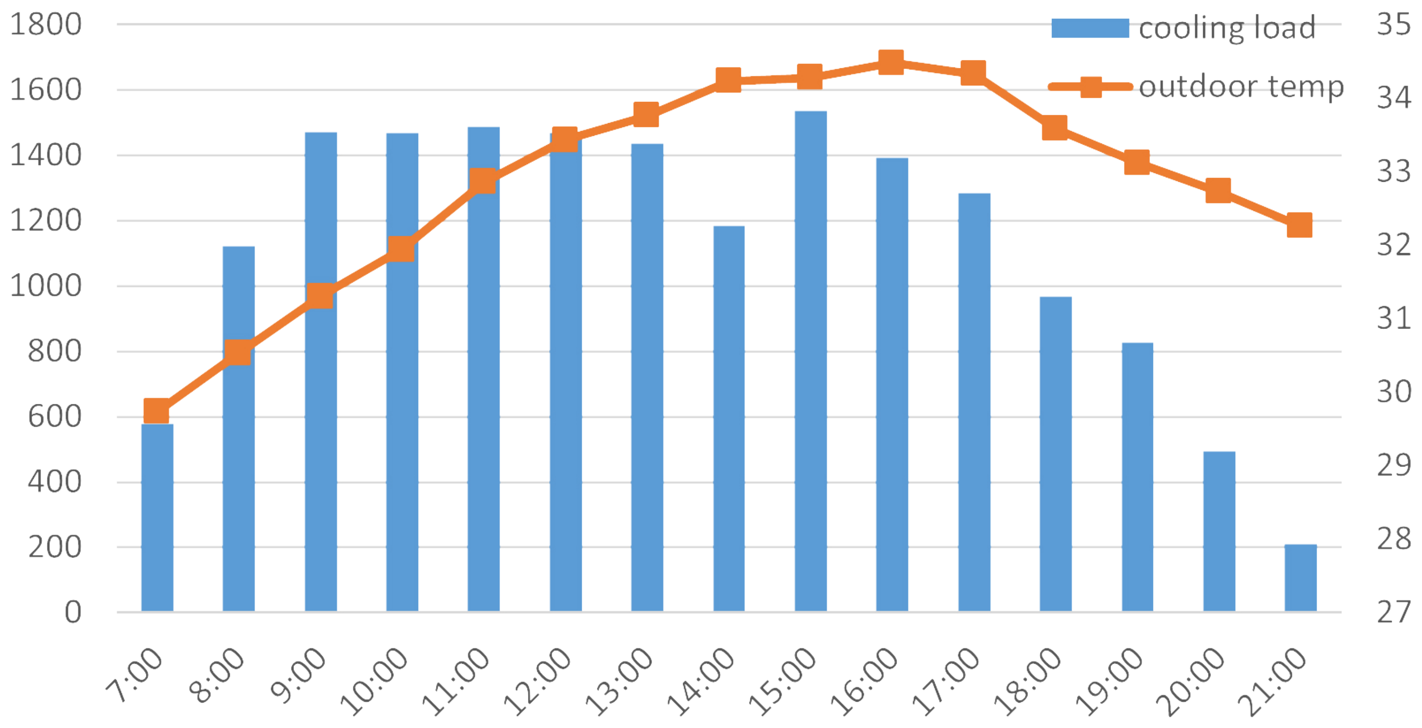
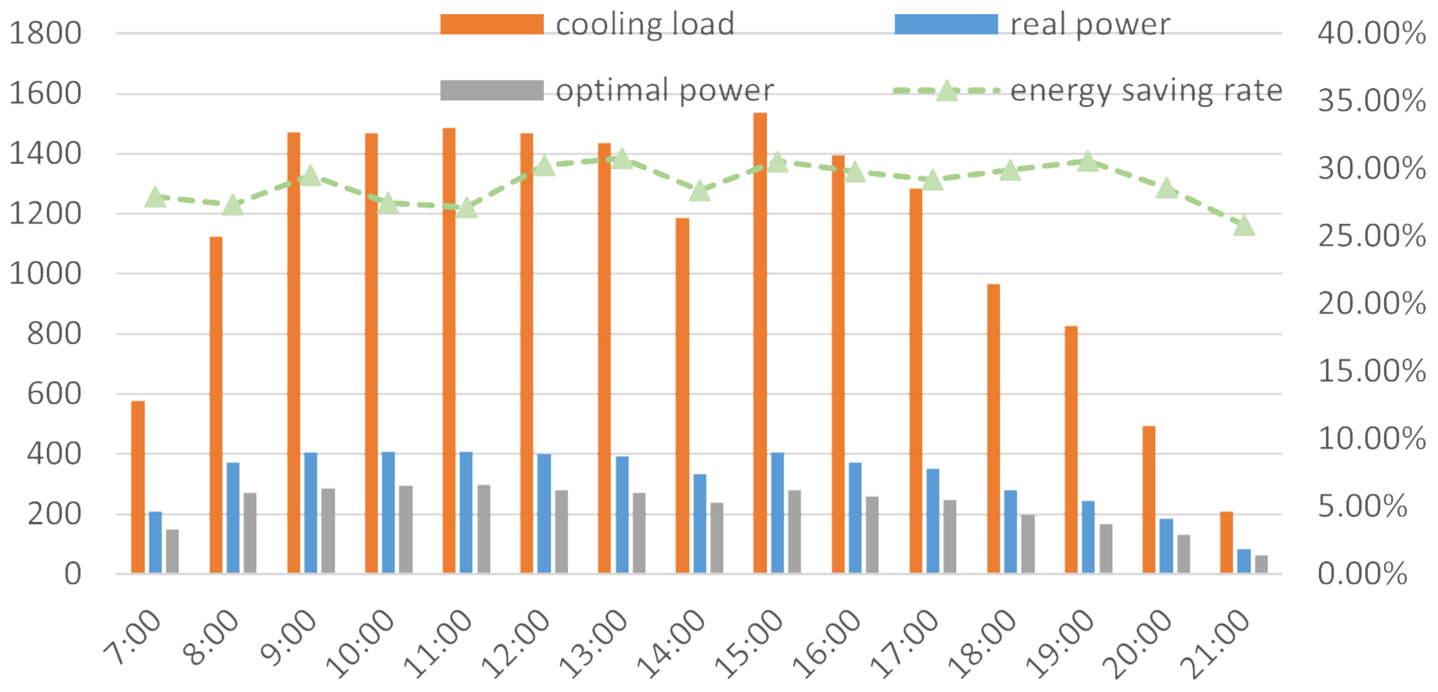
4.3. Typical Day Analysis

The HVAC system in the office building runs from 7 a.m. to 9 p.m. on weekdays and is closed the rest of the time. The switching schedule takes into account the system’s operating requirements and energy-saving. As can be seen from Figure 11, the high load period of the system is from 9 a.m. to 5 p.m., during which there is a large flow of people and a high ambient temperature, which increases the cooling load demand of the building. The ALOE algorithm is used to optimize the energy-saving control of the system throughout the day, and the cooling supply of the system to the building is adjusted according to the actual demand. The experimental results are shown in Figure 11, the HVAC system is expected to save 1412 kWh of electricity, about 565 kg of standard coal, and reduce 1408 kg of carbon dioxide emissions. The overall energy-saving rate of the whole day is 29.06%, and the all-day COP of the system is increased from 3.48 before optimization to 4.91 after optimization, which verifies the effectiveness of the ALOE algorithm in energy-saving optimization of the HVAC system.

5. Conclusions

This study applied various swarm intelligence-based algorithms to explore their potential in optimizing energy-saving for HVAC systems. Using the operational data of an HVAC system from the summer of 2023, a comprehensive model of the HVAC system for an office building in Hangzhou, China, was developed and validated. Various types of swarm intelligence optimization algorithms were used to compare energy-saving optimization effects based on the model. The experimental results under different conditions demonstrated the effectiveness of the Ant Lion Optimizer with Enhancements (ALOE) proposed in this paper, achieving optimal energy-saving rates of 28.16%, 28.26%, and 24.9% under high, medium, and low load conditions, respectively. Finally, the dynamic optimization of the HVAC system for a typical day was performed on the model, showing a total energy-saving rate of 29.06% for the ALOE algorithm. These experimental results validate the superiority and robustness of the proposed algorithm under complex conditions, and this study will contribute to the development of energy-saving and emission-reduction technologies.

In future work, we will conduct more in-depth research in the following directions. First, we will look for more suitable public buildings as research objects to test and validate the algorithm on more complex HVAC systems and a wider range of operational data. Second, we will embed the ALOE algorithm into the existing energy management platform and use the existing Internet of Things system to achieve energy-saving optimization of the HVAC system in actual projects. Finally, more advanced algorithms will be compared to establish a stronger baseline, not just being limited to swarm intelligence algorithms.

References

1. China Association of Building Energy Efficiency. China Building Energy Consumption and Carbon Emissions Research Report (2022). Constr. Archit. 2023, 2, 57–69. [Google Scholar]
2. Miao, Y.; Yao, Y.; Hong, X.; Xiong, L.; Zhang, F.; Chen, W. Research on optimal control of HVAC system using swarm intelligence algorithms. Build. Environ. 2023, 241, 110467. [Google Scholar] [CrossRef]
3. Farahnak, M.; Farzaneh-Gord, M.; Deymi-Dashtebayaz, M.; Dashti, F. Optimal sizing of power generation unit capacity in ICE-driven CCHP systems for various residential building sizes. Appl. Energy 2015, 158, 203–219. [Google Scholar] [CrossRef]
4. Kohlenbach, P.; Ziegler, F. A dynamic simulation model for transient absorption chiller performance. Part I: The model. Int. J. Refrig. 2008, 31, 217–225. [Google Scholar] [CrossRef]
5. Wemhoff, A.; Frank, M. Predictions of energy savings in HVAC systems by lumped models. Energy Build. 2010, 42, 1807–1814. [Google Scholar] [CrossRef]
6. Vakiloroaya, V.; Samali, B.; Madadnia, J.; Ha, Q. Component-wise optimization for a commercial central cooling plant. In Proceedings of the IECON 2011-37th Annual Conference of the IEEE Industrial Electronics Society, Melbourne, Australia, 7–10 November 2011; pp. 2769–2774. [Google Scholar]
7. Park, M.H.; Shin, E.G.; Lee, H.R.; Suh, I.S. Dynamic model and control algorithm of HVAC system for OLEV® application. In Proceedings of the ICCAS 2010, Gyeonggi-do, Republic of Korea, 27–30 October 2010; pp. 1312–1317. [Google Scholar]
8. Terzi, E.; Fagiano, L.; Farina, M.; Scattolini, R. Structured modelling from data and optimal control of the cooling system of a large business center. J. Build. Eng. 2020, 28, 101043. [Google Scholar] [CrossRef]
9. Afram, A.; Janabi-Sharifi, F.; Fung, A.S.; Raahemifar, K. Artificial neural network (ANN) based model predictive control (MPC) and optimization of HVAC systems: A state of the art review and case study of a residential HVAC system. Energy Build. 2017, 141, 96–113. [Google Scholar] [CrossRef]
10. Yao, Y.; Lian, Z.; Hou, Z.; Zhou, X. Optimal operation of a large cooling system based on an empirical model. Appl. Therm. Eng. 2004, 24, 2303–2321. [Google Scholar] [CrossRef]
11. Lu, L.; Cai, W.; Xie, L.; Li, S.; Soh, Y.C. HVAC system optimization—In-building section. Energy Build. 2005, 37, 11–22. [Google Scholar] [CrossRef]
12. Xiaomei, F.; Qifei, J.; Zheng, Z. Analysis on Energy-saving of Year-round Operation Conditions with Variable Flow Cooling Water System. Build. Sci. 2010, 26, 80–84. [Google Scholar]
13. Yang, C.; Gunay, B.; Shi, Z.; Shen, W. Machine learning-based prognostics for central heating and cooling plant equipment health monitoring. IEEE Trans. Autom. Sci. Eng. 2020, 18, 346–355. [Google Scholar] [CrossRef]
14. Krinidis, S.; Tsolakis, A.; Katsolas, I.; Ioannidis, D.; Tzovaras, D. Multi-criteria HVAC control optimization. In Proceedings of the 2018 IEEE International Energy Conference (ENERGYCON), Limassol, Cyprus, 3–7 June 2018; pp. 1–6. [Google Scholar]
15. Barrett, E.; Linder, S. Autonomous hvac control, a reinforcement learning approach. In Proceedings of the Machine Learning and Knowledge Discovery in Databases: European Conference, ECML PKDD 2015, Porto, Portugal, 7–11 September 2015; Proceedings, Part III 15. Springer: Berlin/Heidelberg, Germany, 2015; pp. 3–19. [Google Scholar]
16. Afroz, Z.; Shafiullah, G.; Urmee, T.; Shoeb, M.; Higgins, G. Predictive modelling and optimization of HVAC systems using neural network and particle swarm optimization algorithm. Build. Environ. 2022, 209, 108681. [Google Scholar] [CrossRef]
17. Mirjalili, S. The ant lion optimizer. Adv. Eng. Softw. 2015, 83, 80–98. [Google Scholar] [CrossRef]
18. Wang, L.; Cao, Q.; Zhang, Z.; Mirjalili, S.; Zhao, W. Artificial rabbits optimization: A new bio-inspired meta-heuristic algorithm for solving engineering optimization problems. Eng. Appl. Artif. Intell. 2022, 114, 105082. [Google Scholar] [CrossRef]
19. Rahkar Farshi, T. Battle royale optimization algorithm. Neural Comput. Appl. 2021, 33, 1139–1157. [Google Scholar] [CrossRef]
20. Agushaka, J.O.; Ezugwu, A.E.; Abualigah, L. Dwarf mongoose optimization algorithm. Comput. Methods Appl. Mech. Eng. 2022, 391, 114570. [Google Scholar] [CrossRef]
21. Azizi, M.; Aickelin, U.; Khorshidi, H.A.; Baghalzadeh Shishehgarkhaneh, M. Energy valley optimizer: A novel metaheuristic algorithm for global and engineering optimization. Sci. Rep. 2023, 13, 226. [Google Scholar] [CrossRef] [PubMed]
22. Mohamed, A.W.; Hadi, A.A.; Mohamed, A.K. Gaining-sharing knowledge based algorithm for solving optimization problems: A novel nature-inspired algorithm. Int. J. Mach. Learn. Cybern. 2020, 11, 1501–1529. [Google Scholar] [CrossRef]
23. Askari, Q.; Saeed, M.; Younas, I. Heap-based optimizer inspired by corporate rank hierarchy for global optimization. Expert Syst. Appl. 2020, 161, 113702. [Google Scholar] [CrossRef]
24. Trojovskỳ, P.; Dehghani, M. Walrus optimization algorithm: A new bio-inspired metaheuristic algorithm. Preprint 2022. [Google Scholar] [CrossRef]
25. Amali, D.; Dinakaran, M. Wildebeest herd optimization: A new global optimization algorithm inspired by wildebeest herding behaviour. J. Intell. Fuzzy Syst. 2019, 37, 8063–8076. [Google Scholar] [CrossRef]
26. Terzi, E.; Cataldo, A.; Lorusso, P.; Scattolini, R. Modelling and predictive control of a recirculating cooling water system for an industrial plant. J. Process Control 2018, 68, 205–217. [Google Scholar] [CrossRef]
27. Saxena, P.; Kothari, A. Ant lion optimization algorithm to control side lobe level and null depths in linear antenna arrays. AEU-Int. J. Electron. Commun. 2016, 70, 1339–1349. [Google Scholar] [CrossRef]
28. Reynolds, A. Liberating Lévy walk research from the shackles of optimal foraging. Phys. Life Rev. 2015, 14, 59–83. [Google Scholar] [CrossRef]
29. Yao, X.; Liu, Y.; Lin, G. Evolutionary programming made faster. IEEE Trans. Evol. Comput. 1999, 3, 82–102. [Google Scholar]
30. Jensi, R.; Jiji, G.W. An enhanced particle swarm optimization with levy flight for global optimization. Appl. Soft Comput. 2016, 43, 248–261. [Google Scholar] [CrossRef]
31. Han, X.M.; Qiu, B.; Liu, Q.M.; Zhou, L.Y.; Wang, L.M. Fruit fly optimization algorithm based on Cauchy mutation. Microelectron. Comput. 2017, 34, 26–30. [Google Scholar]
32. Tashtoush, B.; Molhim, M.; Al-Rousan, M. Dynamic model of an HVAC system for control analysis. Energy 2005, 30, 1729–1745. [Google Scholar] [CrossRef]
33. Wijaya, T.K.; Alhamid, M.I.; Saito, K.; Nasruddin, N. Dynamic optimization of chilled water pump operation to reduce HVAC energy consumption. Therm. Sci. Eng. Prog. 2022, 36, 101512. [Google Scholar] [CrossRef]
Figure 1. Full-text structure diagram.
Buildings 14 02842 g001
Figure 2. Algorithm flow diagram.
Buildings 14 02842 g002
Figure 3. Schematic diagram of the operation of the HVAC cooling system.
Buildings 14 02842 g003
Figure 4. Aerial view of the building.
Buildings 14 02842 g004
Figure 5. The HVAC system structure diagram in this case.
Buildings 14 02842 g005
Figure 6. Overview of the HVAC cooling system.
Buildings 14 02842 g006
Figure 7. Chiller PLR-COP characteristic curve.
Buildings 14 02842 g007
Figure 8. Pump Flow-power Characteristic Curve.
Buildings 14 02842 g008
Figure 9. Diagram of cooling load and temperature change under typical day of an office building.
Buildings 14 02842 g009
Figure 10. Comparison chart of the energy-saving effect of the algorithm.
Buildings 14 02842 g010
Figure 11. All day energy-saving optimization effect.
Buildings 14 02842 g011