Research on Vehicle Fatigue Load Spectrum of Highway Bridges Based on Weigh-in-Motion Data

Abstract

Establishing an accurate vehicle fatigue load spectrum is a critical prerequisite for fatigue life analysis and design of highway bridges. However, the time-varying and regional characteristics of vehicle loads pose significant challenges to achieving this goal. This study focuses on vehicle data collected by a weigh-in-motion system installed on a highway bridge in Chongqing, China. The statistical characteristics of vehicle-load-related parameters are analyzed, and the actual vehicle fatigue load spectrum for this section of the road is established. Specifically, vehicles are first categorized based on axle count characteristics. Then, statistical analyses are conducted on key parameters such as vehicle weight, headway time, and axle load for each vehicle type. Finally, the actual vehicle fatigue load spectrum is developed based on Miner’s linear damage rule and the equivalent fatigue damage principle, and the contributions of different vehicle types to fatigue damage are investigated. The results show that the weight distributions of different vehicle types follow a Gaussian mixture distribution, while the headway time distribution for each lane follows a log-normal distribution. A linear approximate relationship was observed between the axle loads of different vehicle types and their respective total weights. Although two-axle trucks exhibited higher frequencies, six-axle trucks contributed the most to structural fatigue damage, accounting for 53.81%. Therefore, six-axle trucks can be regarded as the standard fatigue vehicle model for this section of the road. These findings provide valuable insights for fatigue design and fatigue life assessment of highway bridges under similar vehicle loading conditions.

1. Introduction

In recent years, with the continuous development of the transportation industry, the number and weight of vehicles operating on highway bridges have shown a significant upward trend [1,2]. During operation, highway bridges are subjected to repeated vehicle loads over long periods, leading to the gradual accumulation of fatigue damage, which in turn results in an increasing number of bridge-related accidents year by year [3]. In addressing the issue of bridge fatigue degradation, existing designs typically establish fatigue vehicle models based on standard vehicle load parameters. However, in practical engineering, the time-varying nature of vehicle loads must be considered when diagnosing the service condition and evaluating the remaining life of existing bridges. At the same time, due to the characteristics of vehicles, such as their mass, stiffness, and speed, the load intensity applied to the bridge varies. Particularly for heavy trucks, their larger mass and stiffness can cause significant dynamic effects on the bridge deck during passage, potentially even triggering dangerous resonance phenomena [4,5]. The weigh-in-motion (WIM) system, as an essential component of the bridge structural health monitoring system [6], can monitor vehicle load information in real time, allowing for the early detection of potential safety hazards in bridges [7,8]. Therefore, establishing an accurate vehicle fatigue load spectrum based on the WIM system is of significant importance for fatigue damage analysis of bridge structures.

Previously, numerous scholars, both domestically and internationally, have conducted extensive research on fatigue load spectra or vehicle load models, with foreign research beginning earlier. Schilling et al. [9] used a three-axle fatigue vehicle model with a total mass of 222 kN to accurately reflect the actual fatigue conditions for fatigue design. This model was later incorporated into the AASHTO specifications [10]. Leahy et al. [11] collected vehicle information recorded by WIM systems from 17 locations in 16 states across the United States, compared the loading results of the vehicle load model HL-93, and proposed an improved vehicle model. Van et al. [12] proposed a new vehicle model consisting of three-axle or four-axle trucks based on seven years of vehicle data. In China, research on fatigue load spectra started later but has developed rapidly. Peng et al. [13], based on traffic flow data collected by the WIM system on a cross-sea bridge in Zhejiang, analyzed the vehicle load characteristics for port highway bridges and established a vehicle load spectrum for the section using the equivalent fatigue damage principle. Liu et al. [14] collected vehicle load information from 23 provinces in China and established vehicle fatigue load spectra for highway bridges in each province. The analysis results indicated that six-axle vehicles could be used as the standard fatigue vehicle for most provinces. Subsequently, Liang et al. [2], Rui et al. [15], and Deng et al. [16] carried out similar work and obtained standard fatigue vehicle models for corresponding road sections. Li et al. [1] established a fatigue vehicle load model based on WIM system monitoring data and further calculated the fatigue damage contribution of each vehicle type.

However, despite numerous studies on vehicle fatigue load spectra [17,18], China’s vast territory, along with varying levels of economic development and traffic conditions across regions, means that fatigue load spectra from one area may not be universally applicable. Thus, it is necessary to develop representative vehicle fatigue load spectra based on the specific regional traffic conditions. Furthermore, a large amount of measured vehicle load data indicate that vehicle load parameters (such as vehicle weight, headway, axle load, etc.) exhibit significant randomness, requiring the use of probabilistic and statistical methods for analyzing the measured vehicle load parameters [19,20].

Inspired by the above literature review, this study proposes a vehicle fatigue load spectrum tailored to the local conditions based on vehicle load data collected by the WIM system from a section of a highway bridge. Specifically, the vehicles are classified into six types, and statistical analyses are conducted for vehicle weight, headway, and axle load for each vehicle type using Gaussian mixture distribution models, log-normal distribution models, and regression models, based on the characteristics of the vehicle parameters. Finally, a vehicle fatigue load spectrum is established using Miner’s linear damage rule and the equivalent fatigue damage principle, and the fatigue damage contribution is calculated to derive the standard fatigue vehicle model for the road section.

2. Vehicle Load Data Analysis

2.1. Vehicle Classification

A certain highway bridge in Chongqing is a steel box girder suspension bridge with a span configuration of (247 + 1020 + 280) m. To record vehicle information in real time, the management and maintenance agency installed a WIM system to monitor the vehicles passing over the bridge continuously, as shown in Figure 1. The collected vehicle information includes arrival time, travel lane, speed violation status, travel direction, vehicle speed, vehicle weight, number of axles, axle load, and wheelbase, among other parameters. To understand the traffic conditions of this road section, this study collected vehicle data recorded by the WIM system from 1 November 2022, to 30 October 2023, resulting in a total of 278,233 data entries. It is important to note that during the operation of the WIM system, some vehicle monitoring information was missing due to transmission equipment failures or system maintenance [21].

In addition, the WIM system may experience data distortion due to electromagnetic interference, environmental factors, and human errors. Thus, it is necessary to exclude anomalous vehicle data further. Moreover, when the vehicle load is very low, its impact on the fatigue life of the bridge can be ignored. To simplify the calculations, data from passenger cars and empty trucks, which have minimal impact on the mechanical performance of the bridge structure, are excluded. Based on common vehicle geometric parameters, vehicle weight, speed, and axle load, the following principles were used to process the raw data: ① vehicle weight < 3000 kg; ② wheelbase: first axle distance < 1.5 m, other axle distances < 1 m or >20 m; ③ number of axles < 2; ④ single axle weight <100 kg or > 40,000 kg; ⑤ vehicle speed < 20 km/h or >120 km/h.

After the aforementioned filtering process, unreasonable and excessively small data from the period of 1 November 2022 to 30 October 2023 were excluded, resulting in 64,397 truckload data entries. Considering that structural fatigue damage is mainly controlled by stress amplitude and the number of cycles [22] and that the number of cycles is primarily influenced by the number of vehicle axles, this study roughly classified the vehicles into six types based on the axle count monitored by the WIM system. The proportion of each vehicle type was then calculated, as shown in

Table 1. Amounts and percentages of each truck type.

Vehicle Type Number	Vehicle Type	Schematic Diagram	Amounts	Percentage/%
V2	Two-axle truck		26,010	40.39
V3(A)	Three-axle truck		3962	6.15
V3(B)	Three-axle truck		2718	4.22
V4	Four-axle truck		9252	14.37
V5	Five-axle truck		2468	3.83
V6	Six-axle truck		19,987	31.04

. The results show that the proportions of truck types V2 and V6 are higher than those of other truck types, accounting for 40.39% and 31.04%, respectively. The proportion of truck type V5 is the smallest, at 3.83%. For other trucks, considering that truck type V6 has the highest number of axles and appears more frequently, its impact on the fatigue of the bridge should not be underestimated.

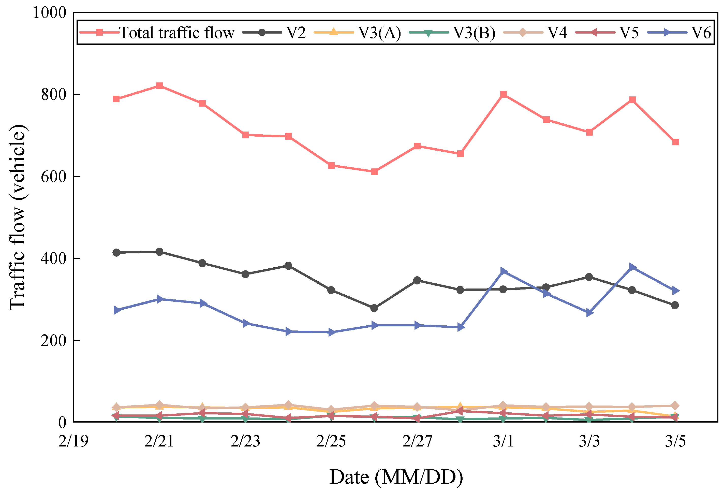
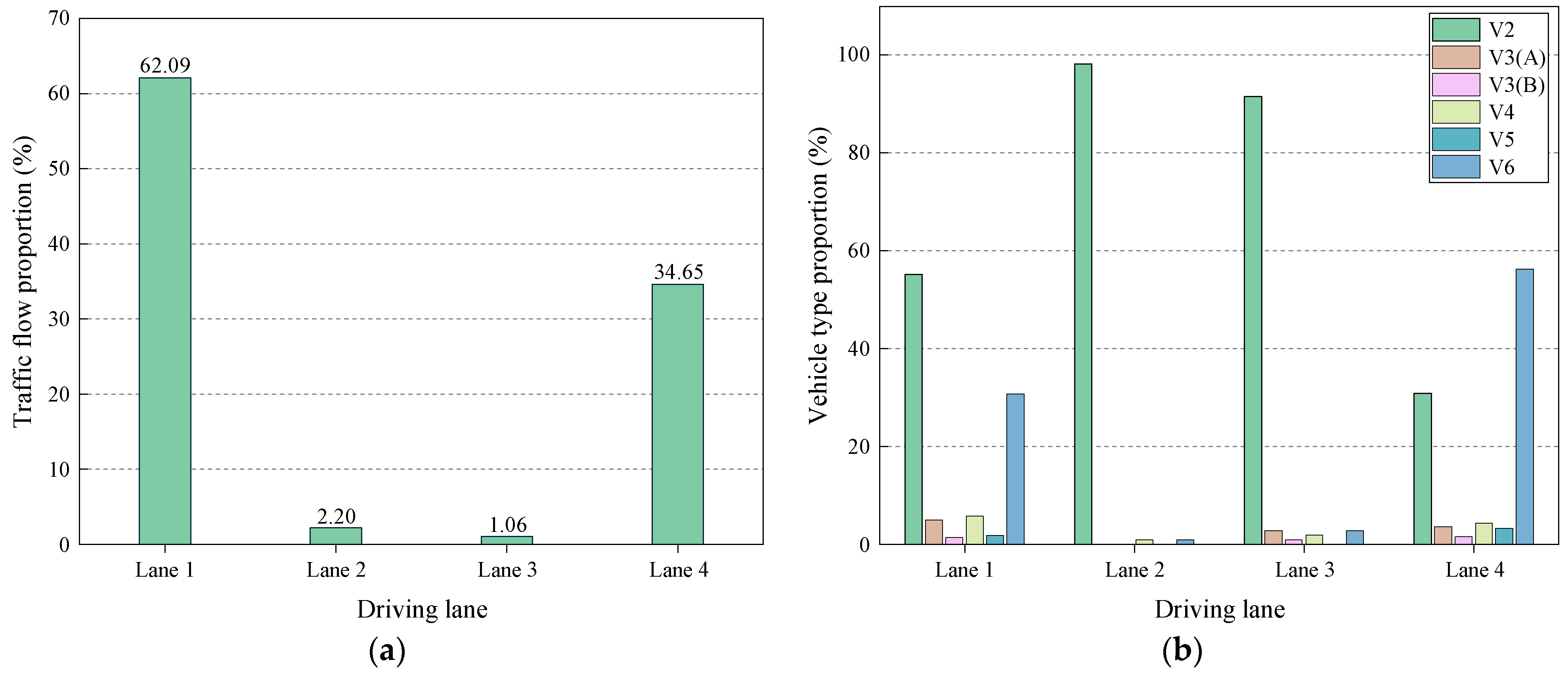
2.2. Traffic Flow Statistics

Due to missing vehicle data during certain periods, only the vehicle data from 20 February to 5 March 2023, spanning two weeks, were analyzed. The traffic flow variation curve for this period was calculated, as shown in Figure 2. From the figure, it is evident that the daily traffic flow fluctuates significantly, with truck types V2 and V6 having higher traffic flow than other vehicle types on each day. Notably, on March 1, March 4, and March 5, the number of V6 trucks crossing the bridge exceeded that of V2 trucks on these days.

Additionally, statistical analysis of the traffic flow during this period was conducted, resulting in the traffic flow and vehicle type distribution for each lane, as shown in Figure 3. From Figure 3a, it can be seen that the highest proportion of trucks is in lane 1 and lane 4, accounting for 62.09% and 34.65%, respectively. The proportion of trucks in the other two lanes (lanes 2 and 3) is less than 3%, as trucks are not allowed to occupy the overtaking lanes (lanes 2 and 3). Moreover, with the increase in axle number and vehicle weight, along with the decrease in vehicle maneuverability, trucks gradually shift from the overtaking lanes to the driving lanes (lanes 1 and 4), resulting in a higher proportion of trucks in the driving lanes.

From Figure 3b, it can be seen that truck type V2 has a higher proportion in lanes 1, 2, and 3 compared to other vehicle types, while truck type V6 has a higher proportion in lane 4 than in the other lanes. Additionally, truck type V2 has a significantly higher proportion in lanes 2 and 3 than in lanes 1 and 4, with the proportion exceeding 90% in lanes 2 and 3. In contrast, three- to six-axle trucks have a higher proportion in lanes 1 and 4 than in lanes 2 and 3.

3. Statistical Parameters of Vehicle Load

3.1. Vehicle Weight

Vehicle weight is one of the most important parameters for evaluating vehicle loads [23]. Structural fatigue damage is primarily controlled by stress amplitude and the number of cycles, with the value of the stress amplitude being mainly influenced by the vehicle weight. Using the vehicle data recorded in Table 1 as the research subject, the vehicle weight for six types of trucks was statistically analyzed. Taking truck type V2 as an example, the weight distribution and its fitted curve based on measured data are shown in Figure 4. From the figure, it can be observed that the weight distribution exhibits a multi-peaked pattern. Therefore, typical models such as Gaussian or log-normal distributions cannot be used to describe it. Existing studies have shown that the probability density of vehicle weight is typically not a single-peaked Gaussian distribution, and in most cases, it shows a multi-peaked distribution [2]. To accurately characterize the weight distribution of different vehicle types, a Gaussian mixture model (GMM) [24] is used to fit the vehicle weight data, and its probability density function is as follows:

$$f(x | n,w,\mu ,\sigma )={\displaystyle \sum _{i=1}^n{w}_i\frac{1}{\sqrt{2\pi }{\sigma }_i}\exp \left[-\frac{{\left(x_i-{\mu }_i\right)}^2}{2{\sigma }_i^2}\right]}$$

(1)

where $n$ represents the number of component types in the GMM distribution; $w_i$ is the weight coefficient, where the sum of all weights equals 1; ${\mu }_i$ and ${\sigma }_i$ are the distribution parameters for the $i\text{-}\mathrm{th}$ component.

The GMM distribution fitting requires determining the number of components in the fitting curve. The more components there are, the better the model’s fitting performance. However, solely using fitting accuracy to assess the quality of the model will inevitably lead to an increase in the number of components, making the model more complex and possibly resulting in overfitting. Thus, it is necessary to find the optimal number of components. The Akaike information criterion (AIC) [25] and the Bayesian information criterion (BIC) [26] are advantageous in terms of simplicity and accuracy and can be used to determine the optimal number of components for a mixture distribution model. The calculation formulas are as follows:

$$\mathrm{AIC}=2n-2\ln L$$

(2)

$$\mathrm{BIC}=n\ln N-2\ln L$$

(3)

where lnL is the maximum likelihood function value of the model, and N is the sample size.

Taking the truck type V2’s weight distribution in Figure 4 as an example, the AIC and BIC values of the GMM distribution for different numbers of components were calculated using Equations (2) and (3), and the results are shown in Figure 5. From the figure, it can be seen that both the AIC and BIC values reach their minimum when the number of components is 8. Therefore, the optimal number of components for the GMM distribution of truck type V2′s weight is 8.

Similarly, using the aforementioned method, the vehicle weight distributions of other trucks were fitted, and the K-S test method (with a significance level of 0.01) was conducted. The frequency histograms and corresponding fitting curves for the three- to six-axle trucks are shown in Figure 6. From the figure, it can be observed that all vehicle types exhibit multiple peaks, with the number of peaks varying. This is due to the rough classification of vehicle types and the differences in cargo capacity among different vehicles. Specifically, the three-axle truck types V3(A) and V3(B) show a three-peak distribution and a four-peak distribution, respectively, with the highest probability densities occurring at vehicle weights of 10.15 t and 14.35 t. Truck type V4 and truck type V6 exhibit a five-peak distribution, with the highest probability densities occurring at vehicle weights of 13.25 t and 18.55 t. Furthermore, in the weight distribution of truck type V5, the distance between peaks is too large, and the highest peak on the far right is relatively low, indicating the presence of some vehicles that are either fully loaded or overloaded. It should be noted that different peaks may correspond to different loading capacities of the trucks. The fitting results for the vehicle weight distribution parameters of these trucks are shown in

Table 2. Vehicle weight distribution parameters of each vehicle.

Vehicle Type Number	Probability Distribution Function	Distribution Parameters
V2	Eight-component Gaussian mixture model	$w_1=0.11$, ${\mu }_1=11.53$, ${\sigma }_1=2.63$ $w_2=0.05$, ${\mu }_2=3.09$, ${\sigma }_2=0.06$ $w_3=0.19$, ${\mu }_3=4.44$, ${\sigma }_3=0.60$ $w_4=0.07$, ${\mu }_4=18.30$, ${\sigma }_4=0.79$ $w_5=0.10$, ${\mu }_5=3.42$, ${\sigma }_5=0.21$ $w_6=0.24$, ${\mu }_6=6.93$, ${\sigma }_6=1.43$ $w_7=0.11$, ${\mu }_7=16.38$, ${\sigma }_7=1.33$ $w_8=0.12$, ${\mu }_8=10.86$, ${\sigma }_8=2.47$
V3(A)	Three-component Gaussian mixture model	$w_1=0.45$, ${\mu }_1=24.74$, ${\sigma }_1=1.33$ $w_2=0.34$, ${\mu }_2=10.17$, ${\sigma }_2=0.77$ $w_3=0.20$, ${\mu }_3=15.64$, ${\sigma }_3=4.48$
V3(B)	Four-component Gaussian mixture model	$w_1=0.19$, ${\mu }_1=16.93$, ${\sigma }_1=5.14$ $w_2=0.25$, ${\mu }_2=14.31$, ${\sigma }_2=0.63$ $w_3=0.33$, ${\mu }_3=25.36$, ${\sigma }_3=1.11$ $w_4=0.23$, ${\mu }_4=22.36$, ${\sigma }_4=2.01$
V4	Five-component Gaussian mixture model	$w_1=0.08$, ${\mu }_1=22.78$, ${\sigma }_1=3.41$ $w_2=0.46$, ${\mu }_2=13.18$, ${\sigma }_2=1.19$ $w_3=0.21$, ${\mu }_3=32.26$, ${\sigma }_3=1.04$ $w_4=0.12$, ${\mu }_4=28.11$, ${\sigma }_4=2.21$ $w_5=0.14$, ${\mu }_5=13.89$, ${\sigma }_5=2.14$
V5	Four-component Gaussian mixture model	$w_1=0.24$, ${\mu }_1=18.04$, ${\sigma }_1=3.32$ $w_2=0.09$, ${\mu }_2=26.65$, ${\sigma }_2=2.90$ $w_3=0.65$, ${\mu }_3=18.24$, ${\sigma }_3=1.39$ $w_4=0.02$, ${\mu }_4=49.38$, ${\sigma }_4=1.90$
V6	Five-component Gaussian mixture model	$w_1=0.07$, ${\mu }_1=18.73$, ${\sigma }_1=3.44$ $w_2=0.40$, ${\mu }_2=47.78$, ${\sigma }_2=1.70$ $w_3=0.09$, ${\mu }_3=33.98$, ${\sigma }_3=7.34$ $w_4=0.34$, ${\mu }_4=18.18$, ${\sigma }_4=1.86$ $w_5=0.11$, ${\mu }_5=43.36$, ${\sigma }_5=3.16$

.

3.2. Headway Time

Headway time refers to the time interval recorded by the WIM system between two consecutive vehicles traveling in the same lane, reflecting the density of traffic flow. Given that small vehicles have a minimal impact on structural behavior, they are typically excluded from fatigue damage calculations. Therefore, this study focuses solely on analyzing the headway time of truck types V2 to V6. Generally, a headway time greater than 3 s between consecutive vehicles is considered to represent a normal operating condition, while a headway time of 3 s or less indicates a congested traffic state. Since small vehicle load data were excluded during the data preprocessing stage, the number of samples with a headway time of less than 3 s is relatively small. Consequently, separately analyzing these two operating conditions would not yield significant insights.

Based on this, this study employs the normal distribution, Weibull distribution, and log-normal distribution to fit the headway time distribution, selecting the best-fitting distribution as the fitting curve for the headway time frequency histogram. The results are shown in Figure 7. As can be seen from the figure, the headway times in lanes 1 and 4 follow a log-normal distribution, with the headway time in lane 1 generally being smaller than those in lane 4. Specifically, the distribution parameters for the headway time in lane 1 are: $\mu =5.18$, $\sigma =1.47$, while the distribution parameters for lane 4 are: $\mu =5.37$, $\sigma =1.52$. Since the number of trucks in lanes 2 and 3 is relatively small (as shown in Figure 3), the headway times between consecutive vehicles are larger, and thus, these lanes are not considered further in the analysis.

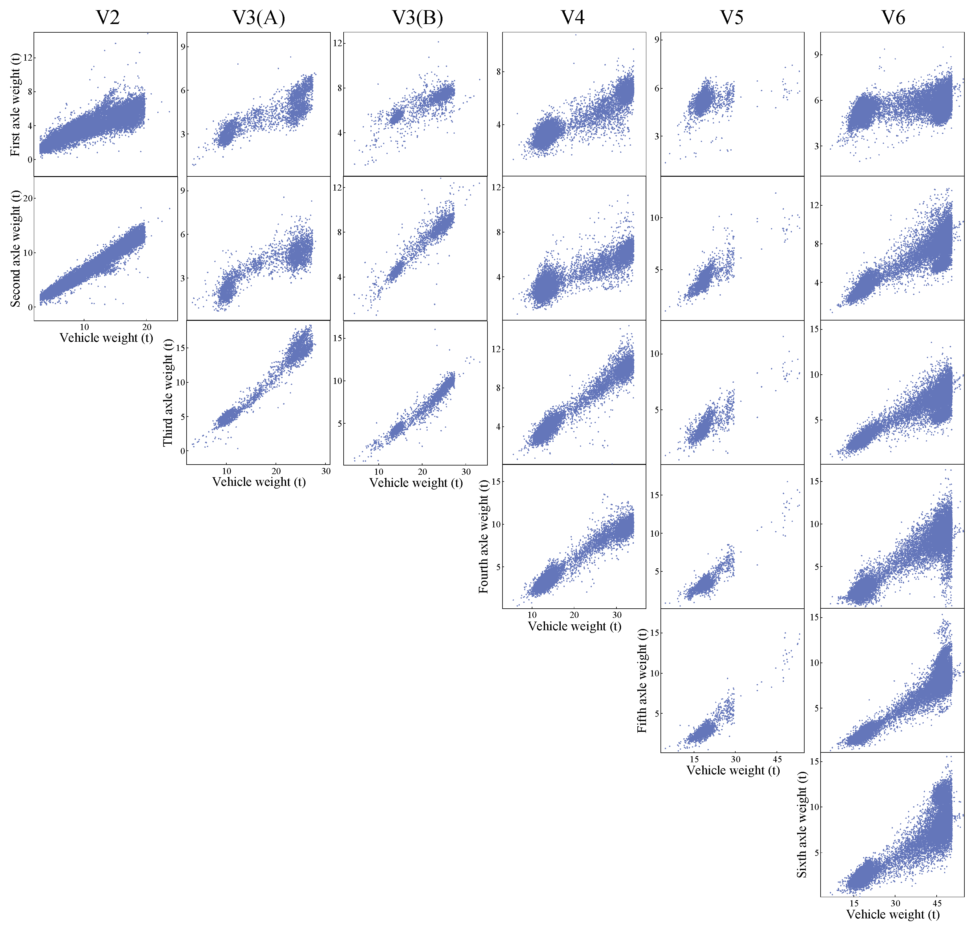
3.3. Axle Load and Wheelbase

For detailed structures and local components, multiple stress cycles are generated when vehicles pass over a bridge. In this case, the stress amplitude and the number of stress cycles cannot be directly calculated from the vehicle weight and lane traffic flow but must be determined based on individual vehicle parameters, namely axle weight and axle spacing. The WIM system can accurately obtain the axle weight and axle spacing of vehicles crossing the bridge. Research has shown that the distribution of axle weights for a vehicle differs from its total weight, but there is a strong linear relationship between them [27]. Therefore, after determining the weight distribution for each vehicle type, it is necessary to establish further the relationship model between each axle weight and the corresponding vehicle weight. In this study, the axles of each vehicle are sequentially numbered from the front to the rear as axles 1 to 6. Using the axle weight data recorded by the WIM system for each truck, a linear regression model is established to describe the relationship between each axle weight and the total vehicle weight. The calculation formula is as follows:

$$y=b_{ij}+a_{ij}x$$

(4)

where y represents the axle weight, and $a_{ij}$ and $b_{ij}$ are the distribution parameters of the vehicle weight.

Figure 8 presents the scatter plots of axle weight versus vehicle weight for truck types V2 to V6. As can be seen from the figure, there is an approximate linear relationship between the axle weight and vehicle weight for different vehicles. Thus, the fitted linear regression equations can effectively represent the relationship between the axle weights and the total vehicle weight for each truck. Furthermore, the distribution parameters for the aforementioned models are provided in

Table 3. The distribution parameters of each axle of different models.

Vehicle Type Number	Axle 1		Axle 2		Axle 3		Axle 4		Axle 5		Axle 6
	ai1	bi1	ai2	bi2	ai3	bi3	ai4	bi4	ai5	bi5	ai6	bi6
V2	0.28	0.74	0.72	−0.74	-	-	-	-	-	-	-	-
V3(A)	0.16	1.27	0.15	1.03	0.69	−2.30	-	-	-	-	-	-
V3(B)	0.20	2.46	0.37	−0.61	0.43	−1.85	-	-	-	-	-	-
V4	0.16	1.08	0.17	0.86	0.34	−0.80	0.33	−1.14	-	-	-	-
V5	0.04	4.45	0.19	0.41	0.17	0.10	0.31	−2.40	0.29	−2.55	-	-
V6	0.02	4.69	0.16	0.31	0.16	−0.08	0.22	−1.62	0.22	−1.77	0.22	−1.53

. As shown in the table, the distribution parameters for axle weight and vehicle weight in each truck are generally similar. For example, in truck type V6, the distribution parameters for axles 4, 5, and 6 are close, with a values all being 0.22 and b values of −1.62, −1.77, and −1.53, respectively. This is likely due to the proximity of the axle spacings, leading to a relatively uniform distribution of axle weights. Based on the table, once the total vehicle weight is known, the axle weights for each axle can be calculated using the linear regression equations.

The axle spacing determines the specific distribution of axle weights on the bridge. However, since the axle spacing of a vehicle is fixed, its range of variation is relatively small. Therefore, in this study, the representative axle spacings for different vehicle types were determined based on the axle spacing data monitored by the WIM system.

4. Analysis of Vehicle Fatigue Load Spectrum

4.1. Vehicle Fatigue Load Spectrum

The vehicle fatigue load spectrum refers to the magnitude of vehicle loads and the frequency of occurrence of each vehicle type that a bridge will experience during its design life. Due to the variety of vehicle types crossing the bridge, the distribution ranges of vehicle weight and axle weight are broad, making it difficult to describe their characteristic data using conventional and deterministic distribution functions. Thus, it is necessary to establish a representative vehicle model for each vehicle type. Based on Miner’s linear criterion and the principle of equivalent fatigue damage [13], the equivalent axle weight for each axle of different vehicle types can be determined. The specific calculation formula is as follows:

$$w_{eq}^{k,j}={\left[{\displaystyle \sum f_i{w}_{ij}^3}\right]}^{{\displaystyle \frac{1}{3}}}$$

(5)

where $w_{eq}^{k,j}$ is the equivalent axle weight of the $j\text{-}\mathrm{th}$ axle of the $k\text{-}\mathrm{th}$ vehicle type; $f_i$ is the frequency of occurrence of the $i\text{-}\mathrm{th}$ vehicle in the $k\text{-}\mathrm{th}$ vehicle type; and $w_{ij}$ is the axle weight of the $j\text{-}\mathrm{th}$ axle of the $i\text{-}\mathrm{th}$ vehicle.

Using Formula (5), the equivalent axle weight for each axle of truck types V2–V6 can be calculated. Next, the total vehicle weight for each truck is the sum of the equivalent axle weights. By combining the frequency of occurrence and axle spacing for each vehicle, the fatigue load spectrum for the highway bridge can be obtained, as shown in

Table 4. Vehicle fatigue load spectrum.

Vehicle Type Number	Vehicle Weight/t	Equivalent Axle Weight/t						Wheelbase/m					Frequency/%
		Axle 1	Axle 2	Axle 3	Axle 4	Axle 5	Axle 6	Axle 1~2	Axle 2~3	Axle 3~4	Axle 4~5	Axle 5~6
V2	11.58	3.99	7.59	-	-	-	-	4.00	-	-	-	-	40.39
V3(A)	19.90	4.44	4.04	11.42	-	-	-	1.90	5.30	-	-	-	6.15
V3(B)	22.23	6.89	7.65	7.69	-	-	-	3.50	1.30	-	-	-	4.22
V4	23.61	4.77	4.86	7.15	6.82	-	-	2.00	5.50	1.30	-	-	14.37
V5	22.60	5.23	4.53	3.88	4.72	4.25	-	3.00	6.00	1.30	1.30	-	3.83
V6	40.50	5.59	6.82	6.34	7.35	7.00	7.40	3.00	1.30	6.50	1.30	1.30	31.04

Note: The frequency in the table refers to the probability of this type of vehicle appearing on the bridge.

.

4.2. Fatigue Damage Contribution

The relative damage impact of vehicles on bridge structures can be reflected by the fatigue damage contribution. Based on the vehicle fatigue load spectrum (Table 4), the fatigue damage contributions of each vehicle type to the bridge structure can be calculated. The peak stress response of the bridge structure is related to the axle weight of each vehicle, so the structural fatigue damage is directly related to the axle weight. The fatigue contribution of each vehicle type can be determined by calculating the fatigue contribution of the equivalent axle weight, which reflects the fatigue contribution of the equivalent vehicle weight. The formula for calculating the fatigue damage contribution caused by the equivalent axle weight of the j-th axle of the k-th vehicle type is as follows:

$${\lambda }_{k,j}={\displaystyle \frac{D_k}{D}}={\displaystyle \frac{p_k{w}_{(eq)k,j}^m}{{\displaystyle \sum _{i=1,h=1}^{k_{\max },j_{\max }}\left(p_i{w}_{(eq)i,h}^m\right)}}}$$

(6)

where ${\lambda }_{k,j}$ is the fatigue damage contribution of the $j\text{-}\mathrm{th}$ axle of the $k\text{-}\mathrm{th}$ vehicle type; $D_k$ is the damage caused by the $k\text{-}\mathrm{th}$ vehicle to the bridge; $D$ is the total damage caused by all vehicles to the bridge; $p_k$ is the frequency of the $k\text{-}\mathrm{th}$ vehicle type; $w_{(eq)k,j}^m$ is the equivalent axle weight of the $j\text{-}\mathrm{th}$ axle of the $k\text{-}\mathrm{th}$ vehicle type; $m$ is the slope corresponding to the S-N curve. According to the relevant study [13], the value used in this study is set to 3.

The fatigue damage contribution rate ${\lambda }_k$ of the $k\text{-}\mathrm{th}$ vehicle type is defined as:

$${\lambda }_k={\displaystyle \sum _{j=1}^{j_{\max }}{\lambda }_{k,j}}$$

(7)

Thus, the fatigue damage contribution of each vehicle and axle to the bridge can be calculated, as shown in

Table 5. The fatigue damage contribution of each vehicle and each axle.

Vehicle Type Number	Number of Axles	Fatigue Damage Contribution/%							Number of Vehicles	Frequency/%
		Vehicle Weight	Axle 1	Axle 2	Axle 3	Axle 4	Axle 5	Axle 6
V2	2	18.55	2.35	16.21	-	-	-	-	26,010	40.39
V3(A)	3	9.26	0.49	0.37	8.40	-	-	-	3962	6.15
V3(B)	3	4.75	1.27	1.73	1.76	-	-	-	2718	4.22
V4	4	11.95	1.43	1.51	4.82	4.19	-	-	9252	14.37
V5	5	1.67	0.50	0.33	0.20	0.37	0.27	-	2468	3.83
V6	6	53.81	4.98	9.01	7.25	11.28	9.76	11.54	19,987	31.04

.

From the above table, it can be observed that: (1) the fatigue damage contribution of the axle 2 weight of truck type V2 is the highest among all vehicle axle weights, accounting for 16.21%, while the fatigue damage contribution of the axle 3 weight of truck type V5 is the lowest, at 0.20%. (2) Although truck type V2 has the highest frequency of occurrence among all vehicle types, the fatigue damage contribution of truck type V6′s weight is the highest, reaching 53.81%. This is because, in the calculation of fatigue damage contribution, the weight of the equivalent axle has a greater weight than the frequency of vehicle occurrence. Additionally, truck type V6 has the most axles, resulting in its equivalent axle weight being higher than that of other vehicles. (3) Due to its lower frequency of occurrence and relatively small equivalent axle weights, truck type V5′s overall fatigue damage contribution is low.

Based on the vehicle fatigue load spectrum and the fatigue damage contribution of each vehicle, it is recommended to select the six-axle truck with the highest fatigue damage contribution as the standard fatigue vehicle for this highway. The total weight of this fatigue vehicle is 40.50 t, as shown in Figure 9.

5. Conclusions

Based on one year of vehicle data monitored by the WIM system on a highway bridge in Chongqing, the vehicles were classified according to their axle group characteristics. The vehicle weight, headway time, and axle load were statistically analyzed, and a fatigue load spectrum for the bridge section was established. Based on this, the fatigue damage contribution of each vehicle type and axle to the bridge was analyzed. The main conclusions are as follows:

(1)

In the traffic flow of vehicles crossing the bridge, the numbers of truck type V2 and truck type V6 account for a larger proportion compared to other vehicle types, with proportions of 40.39% and 31.04%, respectively. Additionally, the distribution of vehicle loads across different lanes is significantly imbalanced, with lanes 1 and 4 having a much higher traffic volume than lanes 2 and 3.

(2)

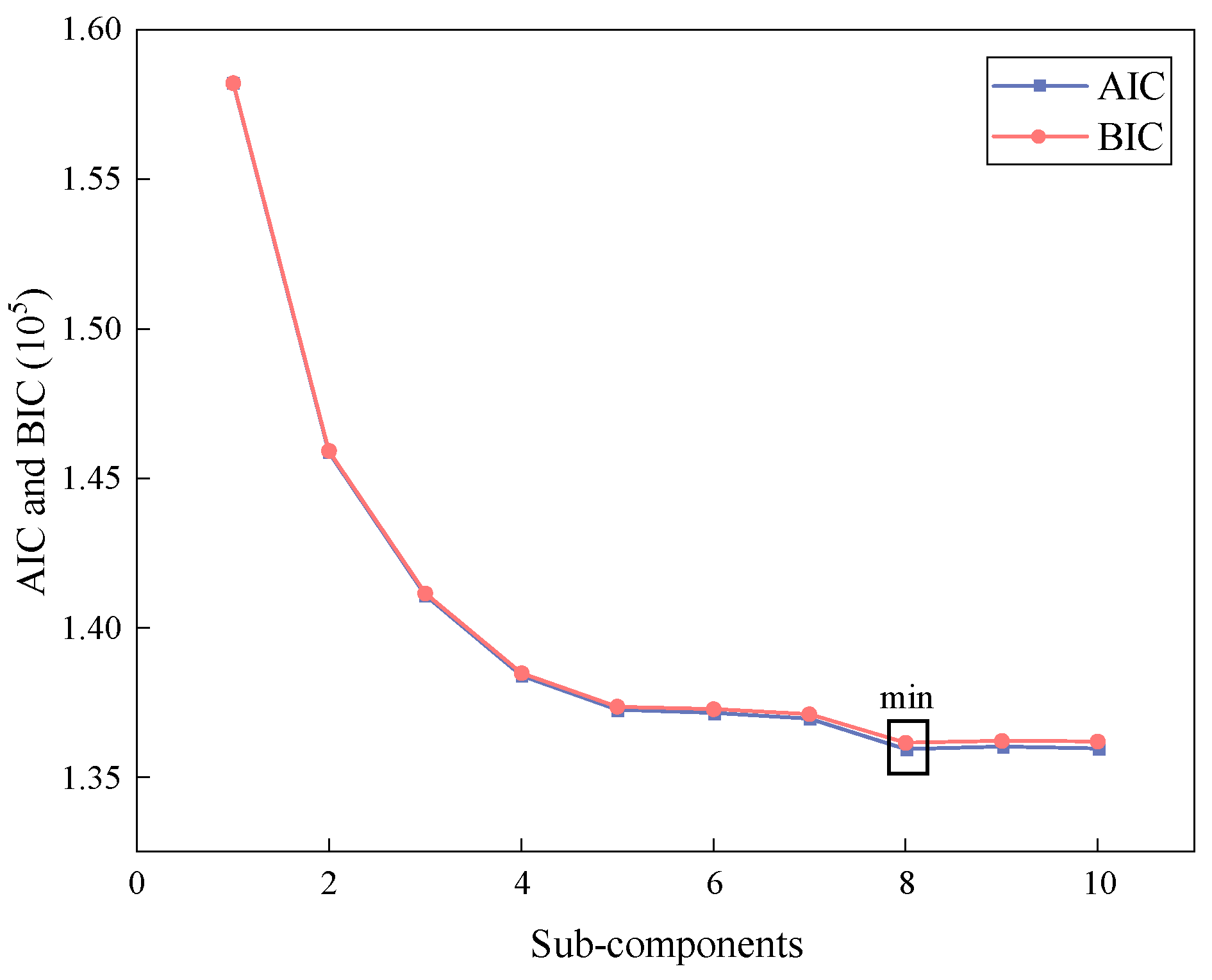
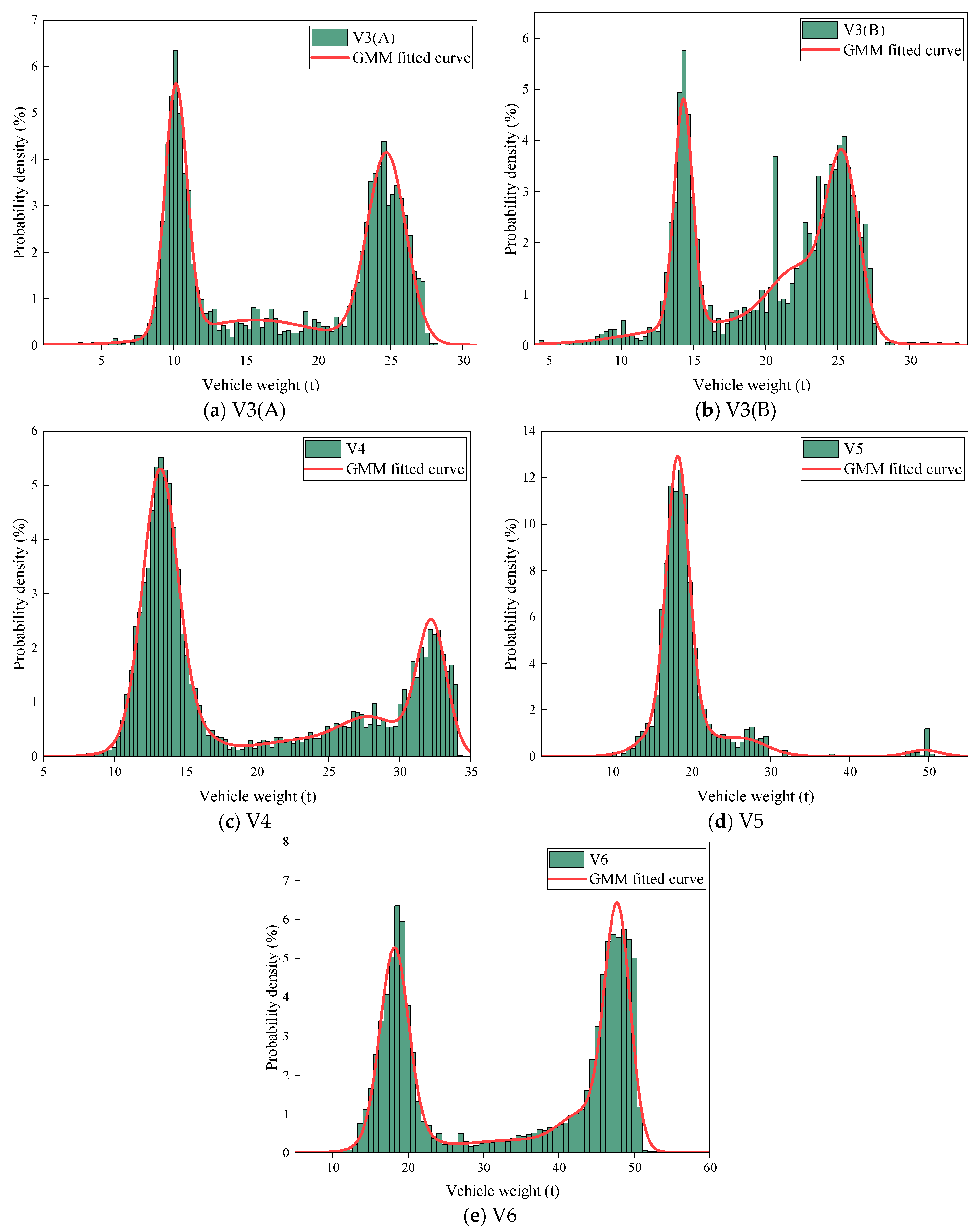
The weight probability density distributions of each truck exhibit a multi-modal pattern. Thus, a GMM was introduced, with the optimal number of sub-components determined using the AIC and the BIC. The results indicate that the weight probability density distributions of truck types V2 to V6 follow Gaussian mixture distributions, which were also validated through the Kolmogorov–Smirnov test. Additionally, the headway time distribution for lanes 1 and 4 can be characterized by a log-normal distribution, and the relationship between axle weight and total vehicle weight for each truck model can be described using a linear regression model.

(3)

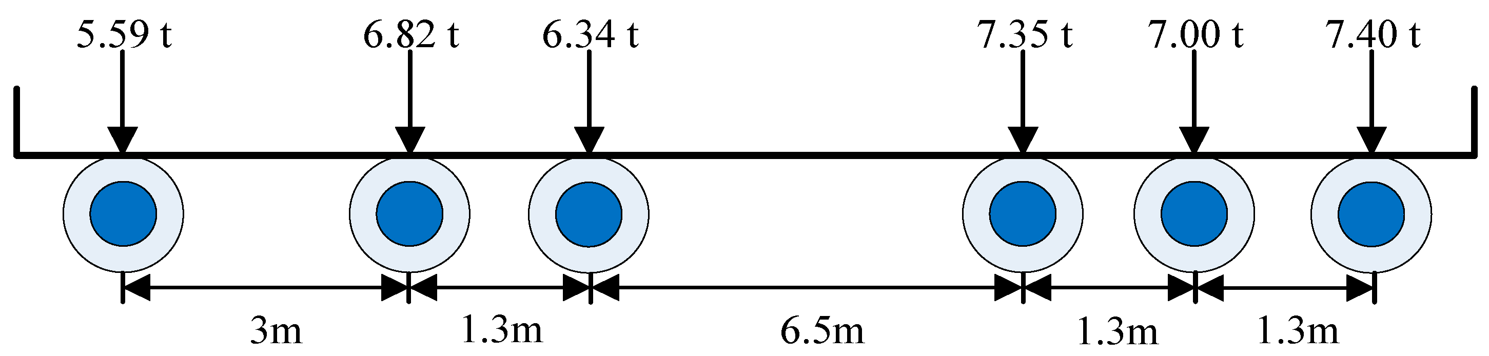
The vehicle fatigue load spectrum reveals that the equivalent vehicle weight for all truck models is greater than 10 t. Among them, truck type V2 has the lowest equivalent weight at 11.58 t, while truck type V6 has the highest equivalent weight at 40.50 t. Additionally, the equivalent vehicle weight tends to increase with the number of axles.

(4)

By calculating the fatigue damage contribution of each axle for each vehicle, it was found that although truck type V2 has the highest frequency, truck type V6 has the greatest fatigue damage contribution to the bridge, accounting for 53.81%. Therefore, based on the vehicle fatigue load spectrum and fatigue damage contribution, it is recommended to select the six-axle truck as the standard fatigue vehicle for this highway.

References

1. Li, M.; Huang, T.L.; Liao, J.J.; Zhong, J.; Zhong, J.W. WIM-Based Vehicle Load Models for Urban Highway Bridge. Lat. Am. J. Solids Strut. 2020, 17, e290. [Google Scholar] [CrossRef]
2. Liang, Y.; Xiong, F. Study of a Fatigue Load Model for Highway Bridges in Southeast China. J. Croat. Assoc. Civ. Eng. 2020, 72, 21–32. [Google Scholar] [CrossRef]
3. Sujon, M.; Dai, F. Application of Weigh-in-Motion Technologies for Pavement and Bridge Response Monitoring: State-of-the-Art Review. Autom. Constr. 2021, 130, 103844. [Google Scholar] [CrossRef]
4. Ling, T.; Deng, L.; He, W.; Cao, R.; Zhong, W. Determination of Dynamic Amplification Factors for Small- and Medium-Span Highway Bridges Considering the Effect of Automated Truck Platooning Loads. Mech. Syst. Sig. Process. 2023, 204, 110812. [Google Scholar] [CrossRef]
5. Carbonari, S.; Nicoletti, V.; Martini, R.; Gara, F. Dynamics of Bridges during Proof Load Tests and Determination of Mass-Normalized Mode Shapes from OMA. Eng. Struct. 2024, 310, 118111. [Google Scholar] [CrossRef]
6. Basu, B.; Bursi, O.S.; Casciati, F.; Casciati, S.; Del Grosso, A.E.; Domaneschi, M.; Faravelli, L.; Holnicki-Szulc, J.; Irschik, H.; Krommer, M.; et al. A European Association for the Control of Structures Joint Perspective. Recent Studies in Civil Structural Control across Europe: Recent Studies in Civil Structural Control Across Europe. Struct. Control Health Monit. 2014, 21, 1414–1436. [Google Scholar] [CrossRef]
7. Mendoza-Lugo, M.A.; Nogal, M.; Morales-Nápoles, O. Estimating Bridge Criticality Due to Extreme Traffic Loads in Highway Networks. Eng. Struct. 2024, 300, 117172. [Google Scholar] [CrossRef]
8. Agüero-Barrantes, P.; Lobo-Aguilar, S.; Hain, A.; Christenson, R.E. Exploring Kriging Metamodeling to Alleviate Speed Reading Dependence in Bridge Weigh-In-Motion Predictions. Structures 2024, 68, 107086. [Google Scholar] [CrossRef]
9. Schilling, C.G.; Klippstein, K.H. New Method for Fatigue Design of Bridges. J. Struct. Div. 1978, 104, 425–438. [Google Scholar] [CrossRef]
10. Norton, T.R.; Mohseni, M.; Lashgari, M. Reliability Evaluation of Axially Loaded Steel Members Design Criteria in AASHTO LRFD Bridge Design Code. Reliab. Eng. Syst. Saf. 2013, 116, 1–7. [Google Scholar] [CrossRef]
11. Leahy, C.; OBrien, E.J.; Enright, B.; Hajializadeh, D. Review of HL-93 Bridge Traffic Load Model Using an Extensive WIM Database. J. Bridge Eng. 2015, 20, 04014115. [Google Scholar] [CrossRef]
12. Van Der Spuy, P.; Lenner, R. Towards a New Bridge Live Load Model for South Africa. Struct. Eng. Int. 2019, 29, 292–298. [Google Scholar] [CrossRef]
13. Peng, X.; Wang, K.; Yang, Q.; Xu, B.; Di, J. Fatigue Load Model of Orthotropic Steel Deck for Port Highway in China. Front. Mater. 2023, 10, 1115632. [Google Scholar] [CrossRef]
14. Liu, Y.; Li, D.; Zhang, Z.; Zhang, H.; Jiang, N. Fatigue Load Model Using the Weigh-in-Motion System for Highway Bridges in China. J. Bridge Eng. 2017, 22, 04017011. [Google Scholar] [CrossRef]
15. Rui, L.; Xiaoyu, X.; Xueyan, D. Fatigue Load Spectrum of Highway Bridge Vehicles in Plateau Mountainous Area Based on Wireless Sensing. Mob. Inf. Syst. 2021, 2021, 9955988. [Google Scholar] [CrossRef]
16. Deng, L.; Deng, Y. Vehicle Load Spectrum and Fatigue Vehicle Model of a Long-Span Concrete-Filled Steel Tube (CFST) Arch Bridge Based on Measured Data of Weight-In-Motion System. Adv. Civ. Eng. 2022, 2022, 3092579. [Google Scholar] [CrossRef]
17. Chen, B.; Zhong, Z.; Xie, X.; Lu, P. Measurement-Based Vehicle Load Model for Urban Expressway Bridges. Math. Probl. Eng. 2014, 2014, 340896. [Google Scholar] [CrossRef]
18. Tian, H.; Chang, W.; Li, F. Development of Standard Fatigue Vehicle Force Models Based on Actual Traffic Data by Weigh-In-Motion System. J. Test. Eval. 2017, 45, 799–807. [Google Scholar] [CrossRef]
19. Chen, B.; Ye, Z.; Chen, Z.; Xie, X. Bridge Vehicle Load Model on Different Grades of Roads in China Based on Weigh-in-Motion (WIM) Data. Measurement 2018, 122, 670–678. [Google Scholar] [CrossRef]
20. Ma, R.; Xu, S.; Wang, D.; Chen, A. Vehicle Models for Fatigue Loading on Steel Box-Girder Bridges Based on Weigh-in-Motion Data. Struct. Infrastruct. Eng. 2018, 14, 701–713. [Google Scholar] [CrossRef]
21. Hasni, H.; Jiao, P.; Alavi, A.H.; Lajnef, N.; Masri, S.F. Structural Health Monitoring of Steel Frames Using a Network of Self-Powered Strain and Acceleration Sensors: A Numerical Study. Autom. Constr. 2018, 85, 344–357. [Google Scholar] [CrossRef]
22. Paepegem, W.V.; Degrieck, J. Effects of Load Sequence and Block Loading on the Fatigue Response of Fibre-Reinforced Composites. Mech. Adv. Mater. Struct. 2002, 9, 19–35. [Google Scholar] [CrossRef]
23. Schmidt, F.; Jacob, B.; Domprobst, F. Investigation of Truck Weights and Dimensions Using WIM Data. Transp. Res. Procedia 2016, 14, 811–819. [Google Scholar] [CrossRef]
24. Ventura, R.; Barabino, B.; Vetturi, D.; Maternini, G. Monitoring Vehicles with Permits and That Are Illegally Overweight on Bridges Using Weigh-In-Motion (WIM) Devices: A Case Study from Brescia. Case Stud. Transp. Policy 2023, 13, 101023. [Google Scholar] [CrossRef]
25. Akalke, H. A New Look at the Statistical Model Identification. IEEE Trans. Autom. Control 1974, 19, 716–723. [Google Scholar]
26. Schwarz, G. Estimating the Dimension of a Model. Ann. Stat. 1978, 6, 461–464. [Google Scholar] [CrossRef]
27. Wang, T. Wind-Vehicle-Bridge Coupled Vibration Analysis Based on Random Traffic Flow Simulation. J. Traffic Transp. Eng. 2014, 1, 293–308. [Google Scholar] [CrossRef]
Figure 1. Layout of the WIM system for a steel box girder suspension bridge.
Buildings 15 00675 g001
Figure 2. Variation curve of traffic flow.
Buildings 15 00675 g002
Figure 3. Traffic flow and vehicle type ratio of each lane. (a) Traffic flow proportion for each lane; (b) Proportion of vehicle types in each lane.
Buildings 15 00675 g003
Figure 4. Frequency histogram and fitting curve of truck V2’s vehicle weight.
Buildings 15 00675 g004
Figure 5. The change curve of information criterion value of truck type V2 mixed distribution model.
Buildings 15 00675 g005
Figure 6. Vehicle weight frequency histograms and fitting curves for each vehicle.
Buildings 15 00675 g006
Figure 7. Headway time frequency histogram and fitting curve of each lane.
Buildings 15 00675 g007
Figure 8. Linear regression models for axle weights and vehicle weights of truck types V2–V6.
Buildings 15 00675 g008
Figure 9. Fatigue load model vehicle.
Buildings 15 00675 g009