Spatiotemporal Dynamics and Driving Factors of Urban Green Space in Texas (2001–2021): A Multi-Source Geospatial Analysis

Abstract

This study investigates the changes in urban green space coverage across 254 counties of varying types in Texas from 2001 to 2021, aiming to explore the spatial patterns of green space transformation and its socioeconomic driving factors. By analyzing Landsat remote sensing data and building type datasets, combined with land use transition matrices, GIS spatial statistics tools, and regression analysis of population and GDP data, this study comprehensively examines the green space change patterns of different urban types. The results indicated significant differences in green space changes across different types of cities: (1) Urban areas with higher populations and rankings, as well as their surrounding regions, show a more pronounced trend of green space converting into built-up urban areas, particularly the expansion of medium and low-density areas. (2) In contrast, green space changes in smaller cities and rural areas occur at a slower pace. Further analysis reveals that the transformation of green spaces is primarily driven by residential land development, with about 39% of green space in high-density urban areas and over 65% in medium and low-density areas being replaced by residential land. (3) The regression analysis results indicate that population growth and GDP growth are the main driving factors for green space changes, explaining up to 86% and 84% of the green space changes, respectively. These findings provide important theoretical support and practical guidelines for urban green space conservation, planning, and sustainable development policies.

1. Introduction

Urban green space typically refers to open and undeveloped land within urban areas that contains green vegetation, such as parks, gardens, street plants, lawns, green roofs, and forests [1]. It can also be defined as urban land fully covered by living green vegetation, including areas like woodlands, grasslands, and shrublands [2,3]. Urban green space is considered one of the most important elements of people’s living environments. With the ongoing process of urbanization, changes in the quantity and quality of urban green spaces have attracted widespread attention in recent years [4,5,6]. Urban green spaces are not only vital sources of ecosystem services, such as air purification, climate regulation, and biodiversity conservation, but also play a crucial role in improving living environments, providing spaces for recreation and psychological health support, and enhancing residents’ overall well-being [7]. Changes in urban green spaces have profound impacts on the health of urban ecosystems and the quality of residents’ lives, directly reflecting shifts in land use. The primary characteristics of these changes include the replacement of green spaces with buildings and impermeable surfaces such as roads and parking lots [8], alterations in ecological functions such as mitigating the urban heat island effect and improving air quality [9], and socioeconomic inequalities emerging over time in the spatial distribution of green spaces [10].

As one of the largest states in the U.S. by land area, Texas has experienced significant population and economic growth over the past two decades, with strong urban expansion dynamics. Its 254 counties exhibit substantial variation in urban classification, economic structure, and natural conditions, making it an ideal case region for observing changes in green space coverage and their main influencing factors [11]. In the state, reports of green space being overtaken by urban land often trigger public concern about ecological environment and quality of life, while government agencies continuously explore legislative and planning strategies to balance development and conservation. This context underscores the necessity and urgency of studying the occupation and transformation of green spaces in Texas.

The launch of the Landsat satellite series has provided researchers with abundant data sources, enabling systematic monitoring of land cover changes [12]. In recent years, machine learning and deep learning methods have been employed for the automated processing of Land Use/Land Cover data (LULC), significantly improving the accuracy and efficiency of land use classification [13]. Based on satellite remote sensing imagery (such as Landsat), the Normalized Difference Vegetation Index (NDVI), and land use/cover data, scholars have described the spatiotemporal patterns of urban green space changes at a macro level, exploring their relationships with socioeconomic, policy, and environmental variables [14,15,16]. For example, Heo et al. examined the link between green space coverage and population health indicators, noting that increased green space significantly improved the physical and mental health of residents [7]. Xing et al. analyzed the imbalance between the supply and demand of green spaces across 102 cities in Hunan Province, China, and applied spatial regression models to assess the impact of economic development on green space distribution [17]. Kitch through a long-term data analysis of 260 U.S. cities, found that high-density built-up areas often face severe green space shortages and emphasized the negative health impacts of green space deficiency on low-income populations [18]. Additionally, Chen revealed significant disparities in accessibility to outdoor green spaces among urban populations in the Global South and North by utilizing high-resolution population distribution and green space data [14]. In the field of environmental and social equity research, an increasing number of studies have focused on the impact of green space on social equity [6,14]. Some scholars point out that the equitable distribution of green space is not only related to environmental protection but also directly influences the quality-of-life differences between social classes [19]. Methodologically, recent studies on urban green space changes and their driving factors have widely utilized remote sensing data analysis, land use modeling, spatial statistical techniques, and regression analysis. For example, Seto et al. employed MODIS imagery to study global urban expansion, emphasizing the extensive impacts of urban growth on ecosystems [20]. Zhu et al. using Landsat data combined with NDVI indices, analyzed green space changes in Guangzhou, China, highlighting uneven distributions of urban green spaces [21]. Additionally, Schinasi et al. applied spatial regression models to explore the influence of socioeconomic variables on green space reduction [22], while Ducey et al. utilized regression analysis to assess the role of population density and GDP on green space dynamics [23]. However, these studies still face certain methodological limitations. Firstly, most research has concentrated on large cities or metropolitan areas [20], lacking systematic comparative analyses across cities of varying sizes. Secondly, quantitative assessments of socioeconomic drivers remain relatively limited, with some studies primarily relying on descriptive analyses [22]. Furthermore, the impacts of medium and low-density urban expansion on green spaces have not been fully explored; many studies mainly focus on high-density urban core areas, neglecting the long-term effects of suburban and low-density expansions on green space [21].

However, existing studies have mainly focused on the “overall change in green space” or “the impact of green space on health and equity”, with less emphasis on the “differentiated processes and uses of green space when it is transformed into various density urban built-up areas”. This research gap somewhat limits our understanding of the mechanisms behind green space transformation, especially since the process and reasons for green space conversion may vary significantly in different types of urban built-up areas [6]. Especially in regions like Texas, which have a vast geographical area and highly heterogeneous internal structures, existing research has mainly focused on macro-level analyses, lacking classification and quantitative analyses of the green space transformation process at the micro level [24,25]. Exploring the relationship between green space occupation and socioeconomic factors, particularly the spatial differences among different urban types, remains a research direction worth investigating. Recent studies have made significant progress in analyzing urban green space changes. For example, Wang et al. used machine learning methods to predict green space changes in the Tokyo metropolitan area, significantly improving the accuracy of data analysis [26]. Haaland and van den Bosch, in their research on European cities, emphasized the importance of green space conservation policies, highlighting the key role of government interventions in mitigating green space conversion [27]. However, these studies still have limitations. For instance, machine learning methods generally exhibit lower interpretability when explaining socioeconomic driving factors [26], and policy-oriented research often lacks specific spatial data support [27].

However, in large-scale rapidly urbanizing areas, there has been a lack of systematic quantitative research on how green spaces are encroached upon by different density urban land uses and the underlying mechanisms involved. Based on the aforementioned research background and literature review, the following key questions can be summarized:

(1)

How does urban expansion affect green space resources in terms of spatial differentiation and use transformation across large geographical regions?

(2)

Do different types of cities exhibit consistent spatiotemporal distribution patterns when green spaces are replaced by low, medium, or high-density urban areas?

(3)

What are the differences in the driving effects of socioeconomic factors (such as population, GDP) and policy orientation on green space occupation and changes across the 254 counties of Texas?

To achieve the stated objectives, this study integrates multi-source data (Landsat remote sensing, building typology, and land use transition matrices) and GIS-based spatial statistical methods. Regression analysis quantifies the contributions of population and GDP growth to green space changes, bridging research gaps across different city types. Additionally, this research focuses not only on large cities but also includes medium-sized, small, and rural areas, aiming to provide tailored policy recommendations for green space planning and protection that align with diverse urban contexts, thereby fostering sustainable urban development.

2. Materials and Methods

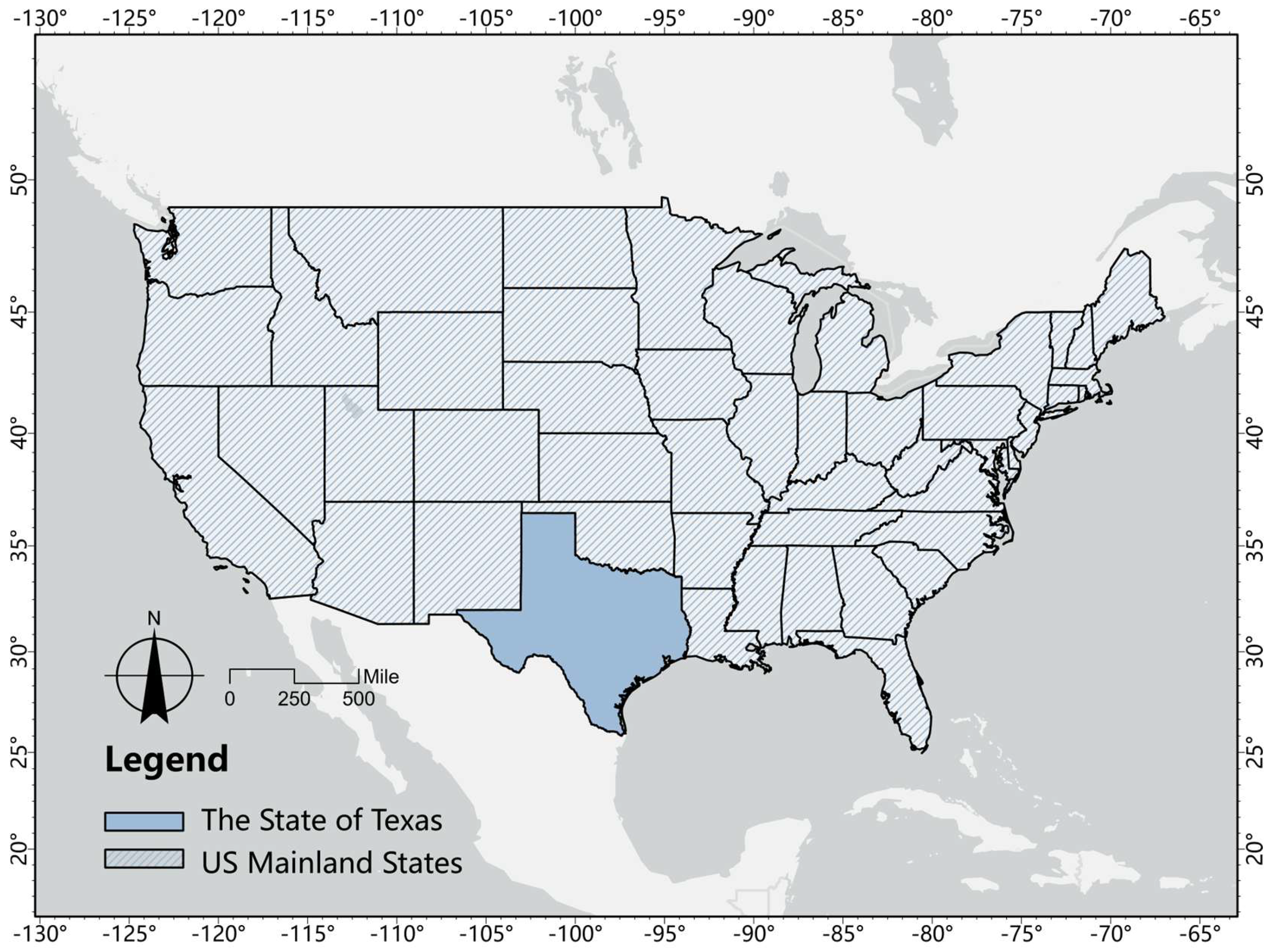
2.1. Study Area: Texas in the Directly Reflecting Shifts in Land Use U.S.

Texas is located in the south-central United States, bordering Louisiana to the east, Arkansas to the northeast, Oklahoma to the north, and New Mexico to the west. It also shares borders with the Mexican states of Chihuahua, Coahuila, Nuevo León, and Tamaulipas and has a Gulf of Mexico coastline in the southeast (Figure 1). The region selected for this study is the entire state of Texas, with the administrative boundaries of its 254 counties serving as the analysis units.

Texas is geographically diverse, with climates ranging from humid subtropical in the east to semi-arid and arid regions in the west. Annual precipitation decreases from over 1200 mm in the east to below 500 mm in the west, while vegetation coverage transitions from dense forests to savannas and desert shrublands [28]. Annual average temperatures range from approximately 10 °C in the north to 27 °C in the south, with summer temperatures exceeding 40 °C in some areas. Extreme weather events, such as droughts, heat waves, and hurricanes, pose challenges to green space changes and urban expansion [3].

As one of the fastest-growing regions in the United States, Texas has experienced nearly 43% population growth since 2000, with an increase of approximately 470,000 residents in 2022 alone [29]. This rapid population growth has driven urban expansion, while relatively permissive land use policies have exacerbated suburban sprawl, increasing infrastructure pressures and significantly impacting the conversion of green spaces [21]. Since the 1980s, a pro-business environment led by the Republican Party has attracted many companies to move in, boosting urban economic prosperity. However, relatively relaxed land use policies have also triggered disorganized suburban sprawl, increasing pressure on infrastructure and public services and significantly influencing the transformation of green spaces [30,31,32].

Therefore, this study focuses on the dynamic transformation of green spaces at the county scale across the entire state of Texas, conducting a systematic analysis based on administrative divisions and related data. The boundary vector files of Texas as a whole and its 254 counties were obtained from the GADM (Database of Global Administrative Areas, https://gadm.org, accessed on 12 January 2025).

2.2. Data Source

2.2.1. Land Use Dataset

Landsat satellite data, characterized by long-term continuity, multispectral capabilities, medium spatial resolution, and free and open access, are widely used in land use/cover research to reveal environmental trends over decades. Specifically, Landsat-8 satellite data utilize the 2–7 spectral bands provided by the Operational Land Imager (OLI) to effectively identify and monitor surface features such as vegetation, water bodies, soil, and buildings (https://www.usgs.gov/landsat-missions/landsat-8, accessed on 12 January 2025). To obtain land use information for different periods in Texas, this study integrated the NLCD 2021 and NLCD 2019 datasets from the USGS National Land Cover Database developed using Landsat-8 satellite data. These datasets use a unified classification scheme for land cover categories and are accessible through Google Earth Engine (GEE).

In the data preprocessing stage, the classification results were merged into 11 major categories for consistent comparative analysis. Finally, TIF format observation data for five periods—2001, 2006, 2011, 2016, and 2021—were selected for the subsequent spatiotemporal change study.

2.2.2. Encroachment Intensity (EI)

To better measure the conversion patterns of green space into urban built-up areas, this study defines the “Encroachment Intensity (EI)” as the degree to which green space is converted to built-up areas, specifically referring to the area of green space converted into built-up land.

Over a five-year scale:

EI = ∑_n − ∑_n−5

Over a twenty-year scale:

EI = ∑_n − ∑_n−20

where “n = 254” represents the sample size of the 254 counties. By calculating both the five-year and twenty-year spans, the study can clearly reveal the phased and long-term impacts of urban expansion on green space.

2.2.3. Urban–Rural Classification

To distinguish between different levels of urban areas, this study adopts the Urban–Rural Classification Scheme for Counties proposed by the National Center for Health Statistics (NCHS) (the related report can be downloaded from https://www.cdc.gov/nchs, accessed on 13 January 2025). This standard divides counties across the country into six categories: large central metro (counties in MSAs of 1 million or more population), large fringe metro (counties in MSAs of 1 million or more population that did not qualify as large central metro counties), medium metro (counties in MSAs of populations of 250,000 to 999,999), small metro (counties in MSAs of populations less than 250,000), micropolitan (counties in micropolitan statistical areas), and noncore (nonmetropolitan counties that did not qualify as micropolitan), which will help identify differences in urbanization levels and green space conversion within Texas in the subsequent analysis.

2.2.4. Population and GDP Data

The population and GDP data for this study primarily come from the United States Census Bureau and the Texas State Library and Archives Commission (available at https://www.tsl.texas.gov/, accessed on 16 January 2025). The population data are derived from both the Population Census and the Population Estimates Program, with key time points including 2000, 2005, 2010, 2020, and 2021. The GDP data are sourced from the U.S. Bureau of Economic Analysis (https://apps.bea.gov/histdatacore/Regional_Accounts_new.html, accessed on 14 January 2025), corresponding to the same time periods as the population data.

2.2.5. Texas Building Typology Dataset

Additionally, to gain a deeper understanding of the detailed functions and expansion processes of urban built-up areas, this study collected building type datasets for Texas. These datasets include information on building types, construction years, and building areas, with each building represented as a polygon (available at https://disasters.geoplatform.gov/USA_Structures/, accessed on 12 January 2025). This data will be integrated with the previously mentioned land use classification to facilitate a more thorough analysis of urban expansion and green space conversion patterns.

2.3. Methods

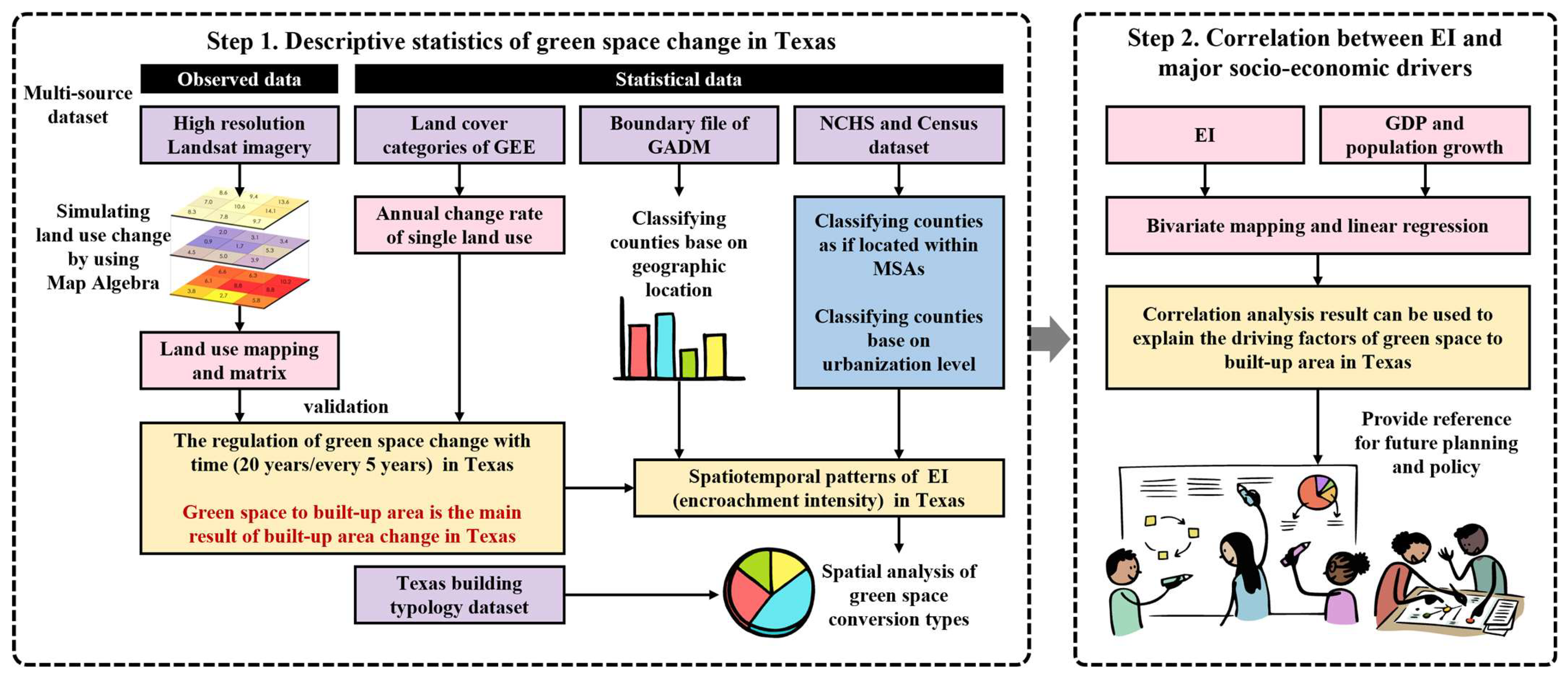
2.3.1. Methodology

This study systematically analyzed the spatiotemporal dynamics and driving factors of urban green spaces in Texas from 2001 to 2021. The process was as follows (Figure 2): first, multi-source data on land use, encroachment intensity, urban–rural classification, population, and GDP were collected; then, a land use transition matrix was built to quantify the transition relationships between different land use types, and a Sankey diagram was used to visually present the evolution patterns; next, the average annual change rates of different land use types were calculated to assess the impact of human activities; then, counties were classified from three dimensions: MSA list, level of urbanization, and geographic location characteristics, to test the spatial differences in the conversion of green spaces to built-up areas; subsequently, in the GIS, the green space change layer was filtered and overlaid with the building dataset to determine the main types of buildings converted from green spaces to built-up areas and to compare their scales and distribution patterns; finally, bivariate mapping and linear regression models were combined to investigate the impact of population and GDP growth on green space encroachment, and the spatial coupling relationships and quantitative relationships were visualized and analyzed to determine whether areas with rapid population and economic growth showed a more significant trend of green space conversion to built-up areas.

2.3.2. Land Use Transition Matrix

The land use transition matrix is a typical application of the Markov model in the quantitative study of land use change. It is used to represent the transition relationships between different land use types at different time periods within a study area. This matrix is widely applied in fields such as land resource management, urban–rural planning, and environmental protection. Typically, the rows of the land use transition matrix represent the land use types at the initial time period (T1), the columns represent the land use types at the subsequent time period (T2), and the matrix elements P_ij represent the total area of land type $i$ converted to type $j$ during the T1–T2 period.

In this study, we combined Landsat data with a resolution of 30 m × 30 m from 2001 to 2021. Using ArcMap software (version 10.8.2) developed by the Environmental Systems Research Institute (ESRI), we employed the raster calculator in the map algebra tool to extract land use type changes for the same pixels across different years (values ranging from 0 to 10, representing different types). From this, we constructed the land use transition matrix. Additionally, to visually present the transitions between land use types, a Sankey diagram was used, providing a more intuitive way to identify and understand the land use evolution patterns across different periods in Texas.

2.3.3. Annual Change Rate of Individual Land Use

To explore the evolution trends of various land use types from 2001 to 2021 (with each phase being 5 years), this study adopts the average annual change rate of a single land use type as a measure of this change. The calculation formula is as follows:

$$\mathrm{A}\mathrm{v}\mathrm{e}\mathrm{r}\mathrm{a}\mathrm{g}\mathrm{e}\mathrm{A}\mathrm{n}\mathrm{n}\mathrm{u}\mathrm{a}\mathrm{l}\mathrm{C}\mathrm{h}\mathrm{a}\mathrm{n}\mathrm{g}\mathrm{e}\mathrm{R}\mathrm{a}\mathrm{t}\mathrm{e}={\displaystyle \frac{\mathrm{C}\mathrm{h}\mathrm{a}\mathrm{n}\mathrm{g}\mathrm{e}\mathrm{i}\mathrm{n}\mathrm{A}\mathrm{r}\mathrm{e}\mathrm{a}\mathrm{o}\mathrm{f}\mathrm{a}\mathrm{S}\mathrm{i}\mathrm{n}\mathrm{g}\mathrm{l}\mathrm{e}\mathrm{T}\mathrm{y}\mathrm{p}\mathrm{e}}{\mathrm{S}\mathrm{t}\mathrm{a}\mathrm{r}\mathrm{t}\mathrm{i}\mathrm{n}\mathrm{g}\mathrm{A}\mathrm{r}\mathrm{e}\mathrm{a}\mathrm{o}\mathrm{f}\mathrm{t}\mathrm{h}\mathrm{e}\mathrm{T}\mathrm{y}\mathrm{p}\mathrm{e}\times \mathrm{Y}\mathrm{e}\mathrm{a}\mathrm{r}\mathrm{I}\mathrm{n}\mathrm{t}\mathrm{e}\mathrm{r}\mathrm{v}\mathrm{a}\mathrm{l}\mathrm{o}\mathrm{f}\mathrm{t}\mathrm{h}\mathrm{e}\mathrm{S}\mathrm{t}\mathrm{u}\mathrm{d}\mathrm{y}\mathrm{P}\mathrm{e}\mathrm{r}\mathrm{i}\mathrm{o}\mathrm{d}\mathrm{C}\mathrm{h}\mathrm{a}\mathrm{n}\mathrm{g}\mathrm{e}\mathrm{i}\mathrm{n}\mathrm{A}\mathrm{r}\mathrm{e}\mathrm{a}\mathrm{o}\mathrm{f}\mathrm{a}\mathrm{S}\mathrm{i}\mathrm{n}\mathrm{g}\mathrm{l}\mathrm{e}\mathrm{T}\mathrm{y}\mathrm{p}\mathrm{e}}}\times 100\mathrm{\%}$$

where Change in Area refers to the increase or decrease in the area of the land type between the current and previous time periods. Starting Area refers to the area of the land type in the previous time period.

This indicator can be used to assess the extent to which human activities have impacted and altered different land use types during various stages, particularly in the context of rapid urbanization, revealing the dynamic changes in land use across different time periods.

2.3.4. Spatial Statistics on Different Types of Urban Green Space Change

To examine the differences in land use change due to urbanization, this study classifies the 254 counties in Texas from three dimensions:

(1)

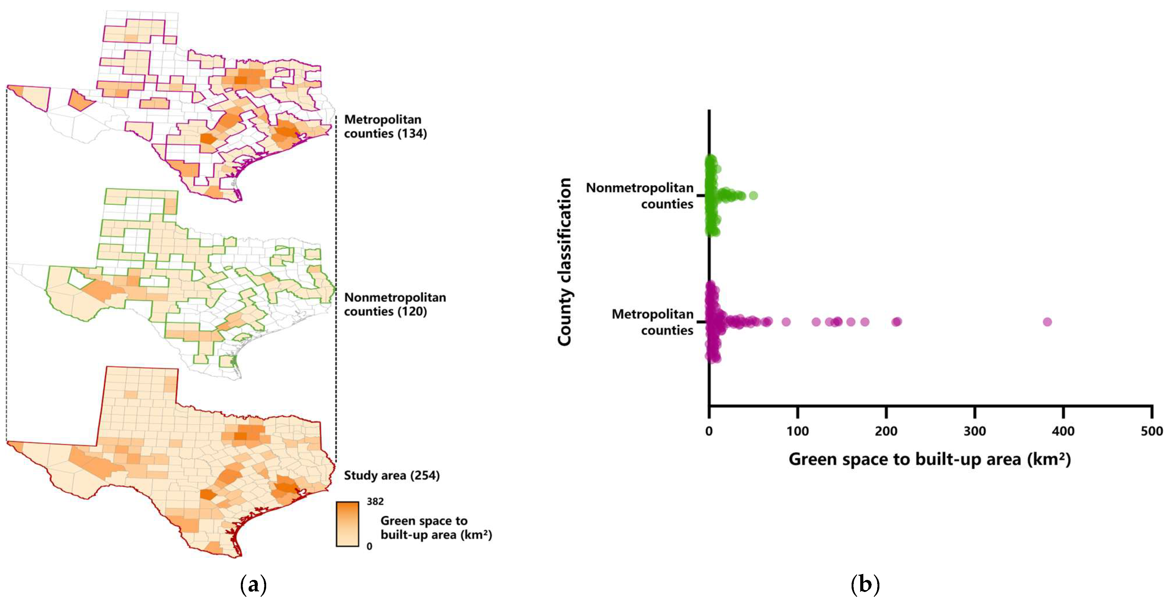
MSA vs. Non-MSA: According to the U.S. government’s definition of Metropolitan Statistical Areas (MSAs), counties within an MSA are categorized as one group, while the remaining counties are classified as another. Numerous studies have shown that MSA regions typically exhibit more prominent urbanization, higher population growth, and greater economic development, all of which have a more pronounced impact on land use change, especially green space conversion.

(2)

Different Urbanization Levels: This study adopts a county classification method currently used by the American Cancer Society (ACS). When conducting cancer screening and differential reporting across the United States, the American Cancer Society uses this classification and naming approach. Based on this, counties are classified into different levels of urbanization, such as large metropolitan counties, small-to-medium metropolitan counties, and nonmetropolitan counties [33].

(3)

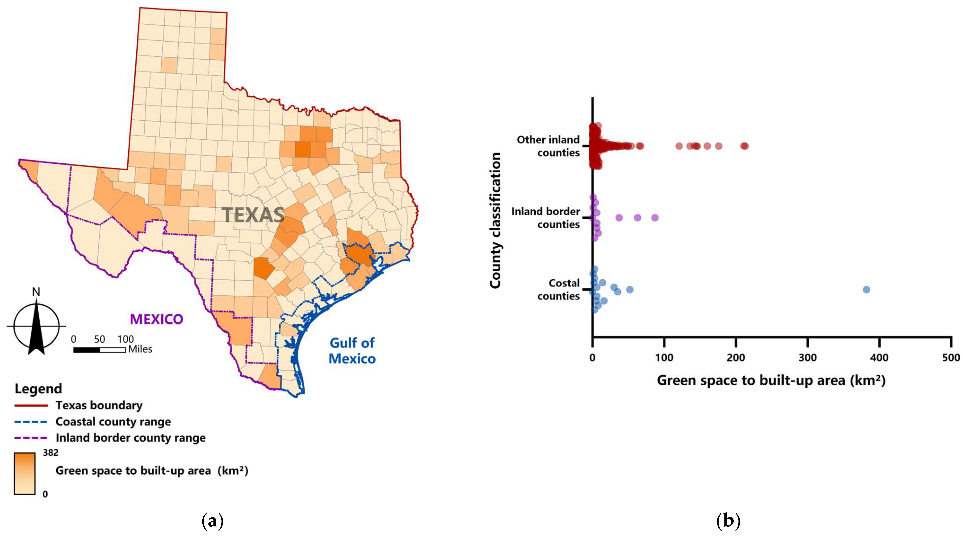
Geographic Location Characteristics: The 254 counties are divided into three categories based on geographic characteristics as follows: coastal counties (those bordering the Gulf of Mexico), inland border counties (those bordering the Mexican border), and other inland counties.

This classification is used to investigate the differences in green space conversion patterns under different geographical conditions. For both of these classification variables, the study tests whether there are significant spatial differences in the conversion of green spaces to built-up areas.

2.3.5. GIS-Based Spatial Analysis of Green Space Conversion Types

Using GIS analysis tools, the green space change layer was first filtered. This layer was then overlaid with the Texas building dataset to determine the main building types converted from green space to built-up areas using the “building centroid localization” method. The process involves the following steps:

(1)

Calculating the geometric centroid of each building using ArcGIS 10.8.

(2)

Applying the “Select by Location” tool with the spatial relationship set to “Center within features,” where features in the input layer are selected if their centers fall within a chosen feature (for polygons and multipoints: geometric centroid is used; for line inputs: midpoint of the geometry is used).

This method establishes the spatial relationship between building centroids and built-up areas. By avoiding traditional polygon intersections, it eliminates issues like duplicate classification and attribution ambiguity, ensuring each building is uniquely associated with one built-up area density attribute. This significantly enhances the accuracy of spatial analysis and classification results.

Based on this, the study further compares the scale and distribution patterns of green space conversion to “high, medium, and low-density” built-up areas (three density classes of built-up areas are extracted from NLCD based on impervious surface coverage; however, the specific parameters are not publicly available), quantifying the changes in land use structure in Texas under the backdrop of rapid urbanization.

2.3.6. Bivariate Mapping and Linear Regression

To further explore the impact of population and GDP growth on green space encroachment by built-up areas, this study combines bivariate mapping and linear regression models. The bivariate mapping tool in ArcGIS Pro was used to visualize the spatial coupling relationships between population growth, GDP growth, and green space encroachment intensity at the county-level scale. By overlaying color gradients, this method identifies spatial consistency between high-growth and high-encroachment areas. Population growth and GDP growth are continuous variables, while green space encroachment intensity is also a quantitative indicator, making them suitable for linear regression analysis based on variable type requirements. Additionally, when constructing linear regression models for population growth, GDP growth, and the intensity of green space encroachment, respectively, several observed outliers were excluded. These outliers might be due to potential data collection errors or the occurrence of extreme events. Eventually, the sample sizes were n = 253 and n = 251, respectively (the original sample size was n = 254). A linear regression model is applied for statistical testing to determine whether areas with rapid population and economic growth show a more significant conversion of green space to built-up areas and to investigate the underlying mechanisms.

3. Results

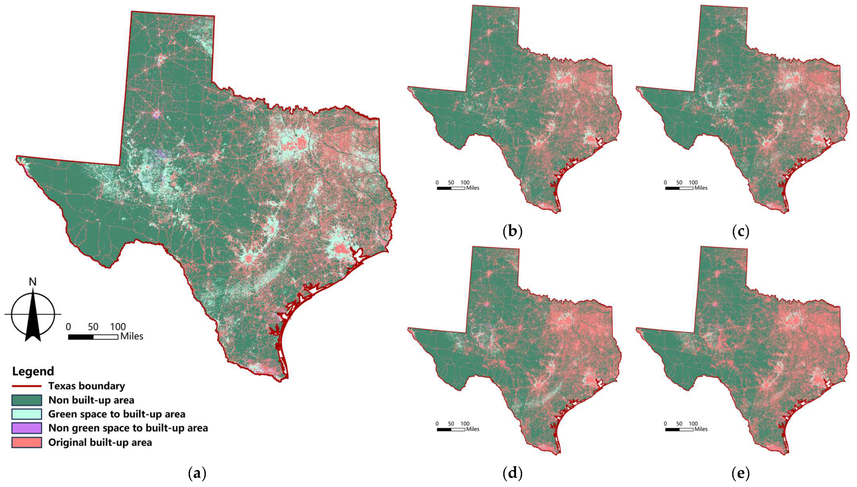
3.1. Transitions Between Green Space and Built-Up Areas

In 2021, of the approximately 24,957 km² of built-up land in Texas, about 18,618 km² was existing built-up area, while approximately 4085 km² came from the conversion of previous green spaces, becoming the main source of green space change (Figure 3). A comparison of remote sensing images from 2001, 2006, 2011, 2016, and 2021 reveals the significant expansion of built-up areas around major cities such as Dallas, Houston, and Austin. This expansion is accompanied by a noticeable reduction and fragmentation of green spaces, particularly around the urban core areas.

The results of the period-based statistical analysis are as follows:

(1)

2001–2006: Built-up areas increased slightly, with major expansion occurring around large cities.

(2)

2006–2011: The expansion rate accelerated, with surrounding green spaces and agricultural land being significantly occupied.

(3)

2011–2016: The urban boundary continued to expand, and the reduction of green spaces persisted.

(4)

2016–2021: The urbanization process intensified, and the newly added built-up areas continued to occupy green and agricultural land at a high intensity.

The flow chart (Figure 4) based on data from different time periods shows the conversion of green spaces and agricultural land into urban built-up areas, reflecting the profound impact of urbanization on land use patterns. Notably, the flow of green space into urban land is significantly wider than other conversion paths, indicating a larger scale of occupation. In certain areas, there is also some degree of mutual conversion between different types of green spaces (such as grasslands, shrublands, and forests); however, the overall scale is relatively small and not as prominent compared to the trend of green space reduction driven by urban expansion.

From the statistical results of changes in a single land use (2001–2021) shown in Figure 5, it can be observed that, after 2016, certain types of green space may show a slight increase in localized areas. However, overall, the decreasing trend remains. The change rate over five-year intervals also indicates that, in the later periods, fluctuations in the increase and decrease in green space became more pronounced in some regions.

3.2. The Encroachment of Green Space in Different County Classifications

3.2.1. Classification of Counties by MSA List

After classifying counties into metropolitan and nonmetropolitan categories based on the Metropolitan Statistical Area (MSA) list, it was found that green space encroachment was more pronounced in metropolitan areas, which appeared as darker fill colors in multi-layer overlay analysis maps (Figure 6). Additionally, built-up area increases in some counties were concentrated in former green spaces (

Table 1. Intensity of green space to built-up area in the classification of the MSA list of counties.

		Metropolitan Counties	Nonmetropolitan Counties
Descriptive statistics	Classification rules	Counties situated within MSAs	Counties outside of MSAs
	Number of counties	134	120
	Total land (km2)	341,039	345,174
	Total change (km2)	3385	706
	Intensity of changes	1.0%	0.2%
Differentiation analysis	Mann–Whitney test	p value < 0.001

).

3.2.2. Classification of Counties by Urbanization Level

After classifying counties into large metropolitan counties (populations over 1 million), small-to-medium metropolitan counties, and nonmetropolitan counties by urbanization level, it was found that green space encroachment was more pronounced in metropolitan areas, which appeared as darker fill colors in multi-layer overlay analysis maps (Figure 7). Additionally, it was observed that built-up area increases in some counties were concentrated in former green spaces (

Table 2. Intensity of green space to built-up area in the classification of the urbanization level of counties.

		Large Metropolitan Counties	Small-to-Medium Metropolitan Counties	Nonmetropolitan Counties
Descriptive statistics	Classification rules	Counties situated within MSAs with populations exceeding one million	Counties situated within MSAs with populations below one million	Counties outside of MSAs
	Number of counties	6	128	120
	Total land (km2)	17,452	323,587	345,174
	Total change (km2)	1209	2175	701
	Intensity of changes	6.9%	0.7%	0.2%
Differentiation analysis	Kruskal–Wallis test	p value < 0.001

).

3.2.3. Classification of Counties by Geographic Location

After classifying the 254 counties in the state into coastal counties, inland border counties, and other inland counties, the area of green space converted into built-up areas showed a certain degree of accumulation. Among the three types of counties, some counties had more than 10 km² of green space occupied by built-up areas; however, overall, no particularly significant differences were observed (Figure 8). Coastal counties exhibited a slightly more concentrated distribution for this indicator, and the other two types of counties also showed similar trends (

Table 3. Intensity of green space to built-up area in the classification of the location of counties.

		Coastal Counties	Inland Border Counties	Inland Counties
Descriptive statistics	Classification rules	Counties located along the coastline	Counties located inland and along the U.S.-Mexico border	Counties located inland but not along the U.S.–Mexico border
	Number of counties	16	12	226
	Total land (km2)	37,258	80,674	568,281
	Total change (km2)	564	221	3300
	Intensity of changes	1.5%	0.3%	0.6%
Differentiation analysis	Kruskal–Wallis test	p value = 0.2592

).

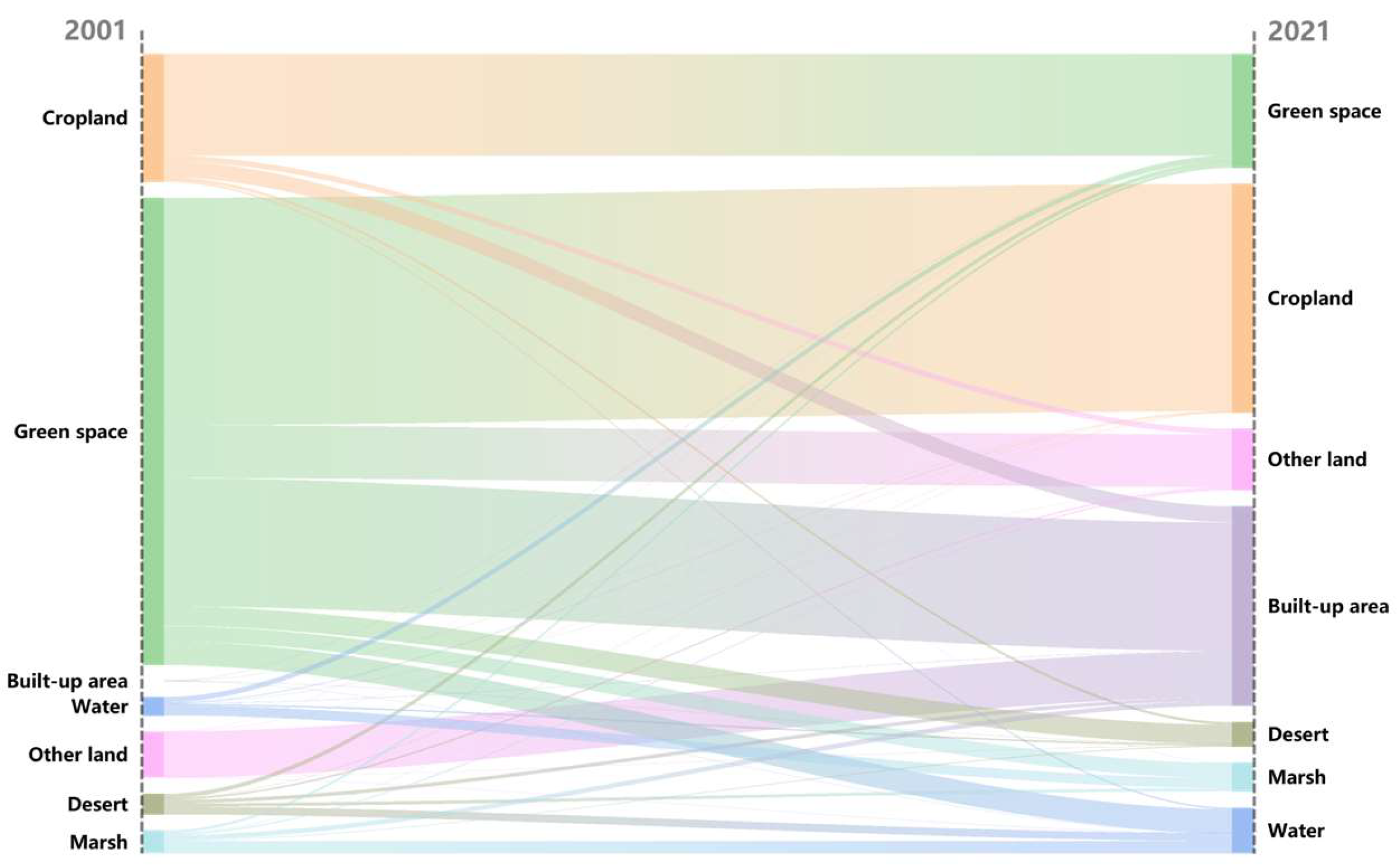
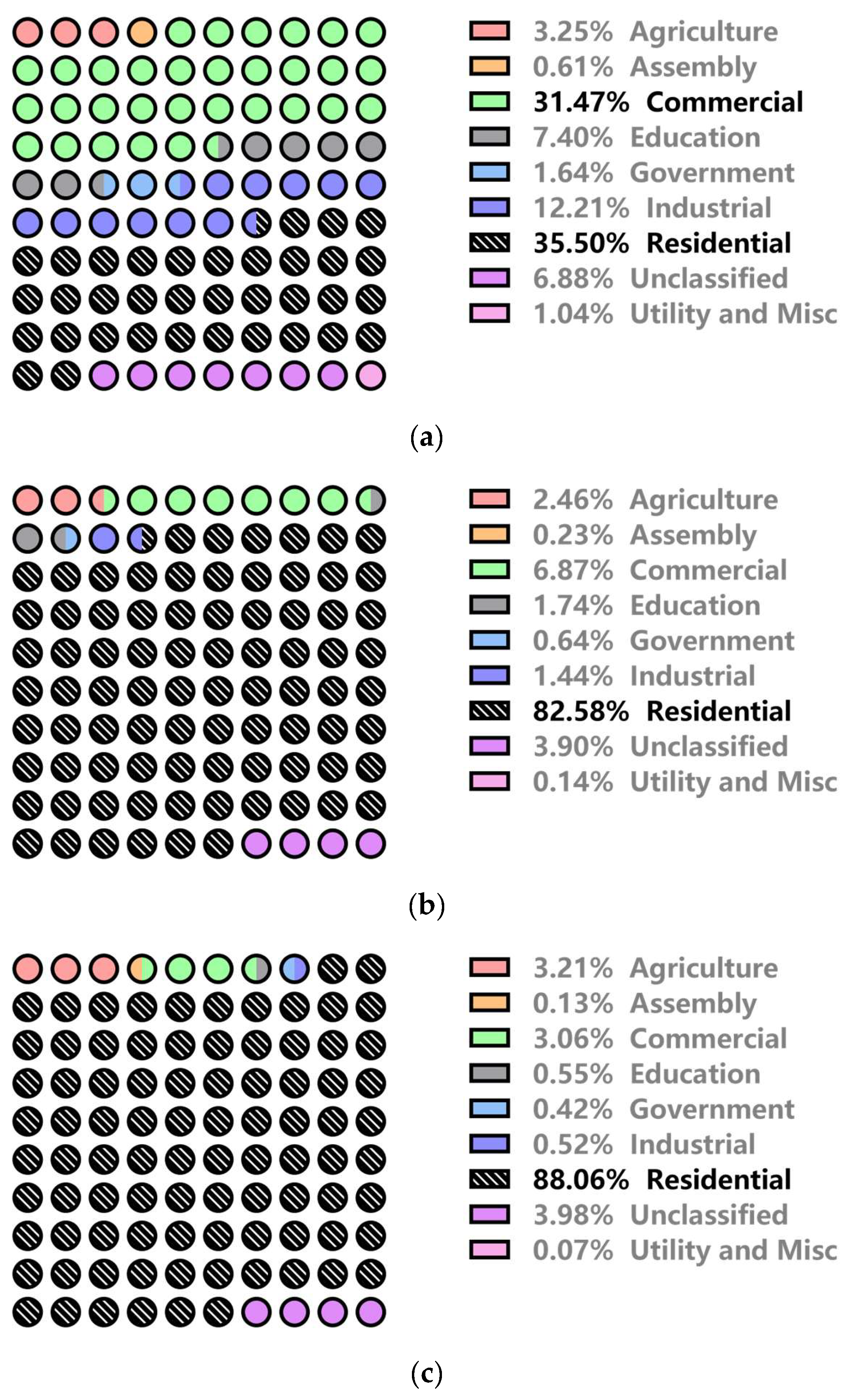
3.3. Types of Green Space Occupied by Urban Built-Up Areas

Statistics on land use conversion of green space over the past 20 years show that residential land has the highest proportion of occupation in medium and low-density built-up areas, making it the primary direction of green space occupation in urban expansion. In high-density built-up areas, both commercial and residential land contribute to the reduction of green spaces, indicating that the development of high-density areas often involves buildings with mixed functions (Figure 9).

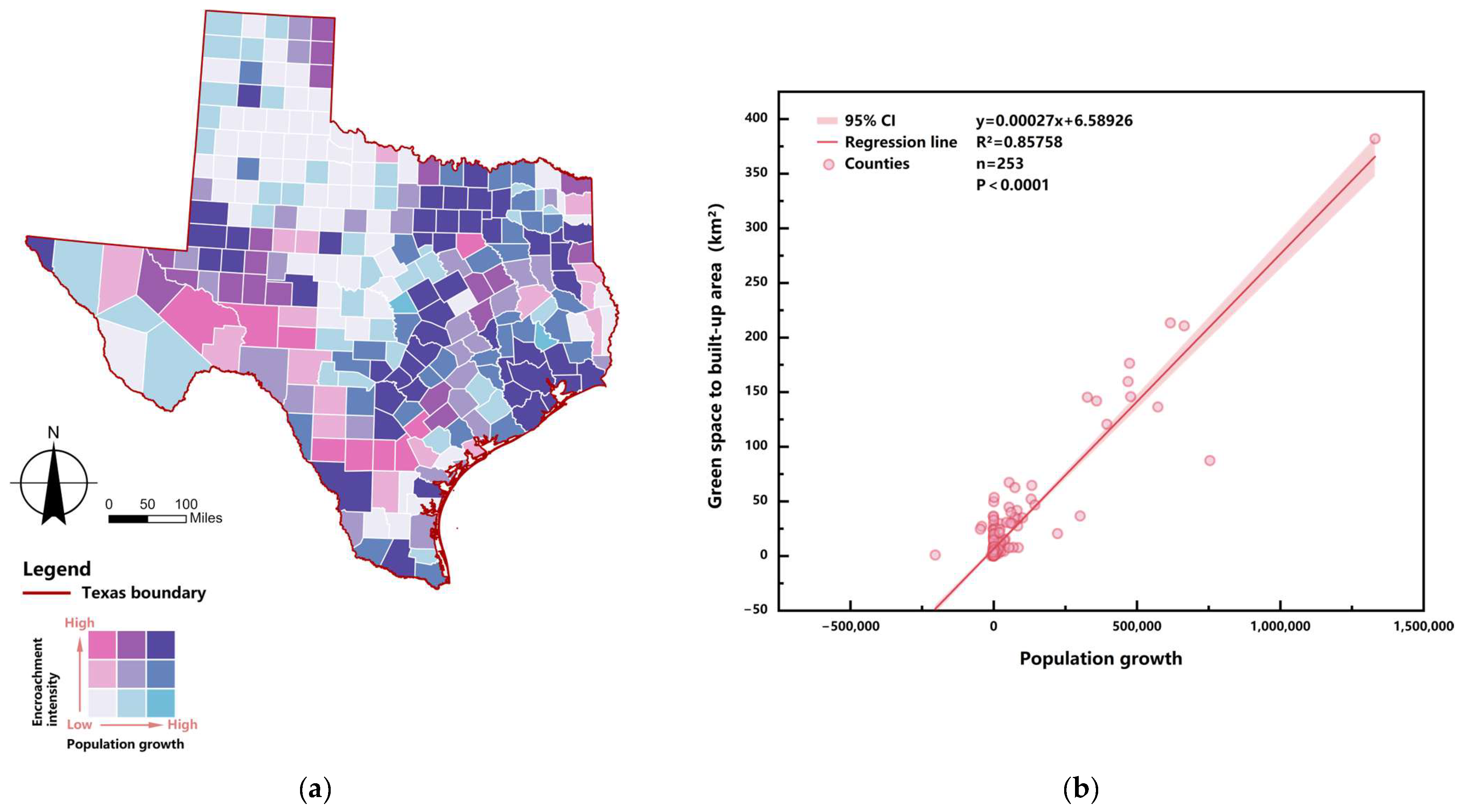
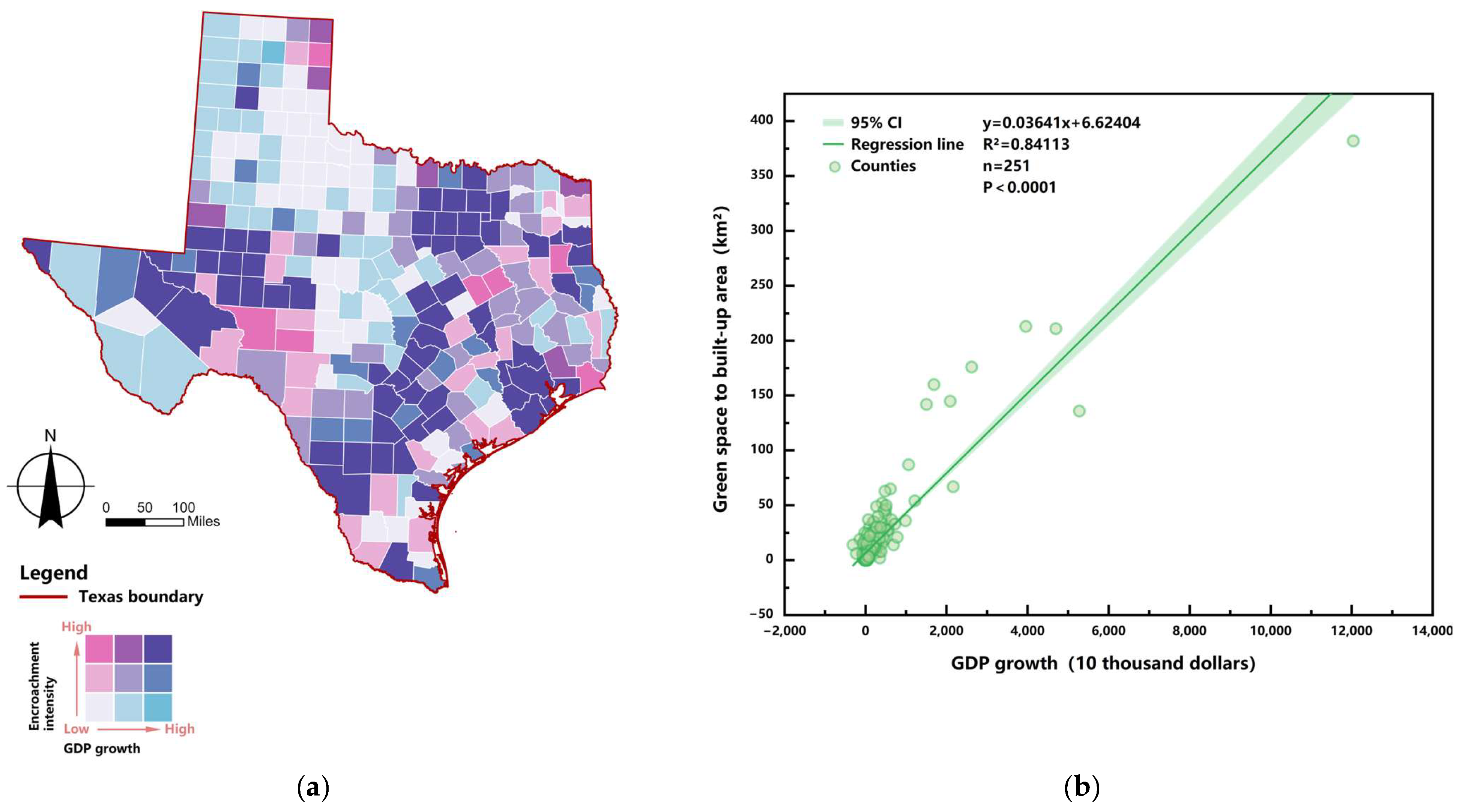
3.4. Bivariate Choropleth Map and Linear Regression

In the bivariate mapping, population/GDP changes in county-level regions show a positive correlation with green space reduction. Areas shown as high–high in the color overlay gradient classification are primarily concentrated in counties of metropolitan areas such as Dallas, Houston, and Austin. Linear regression analyses of population change vs. green space reduction (R² ≈ 0.86, p < 0.001) and GDP change vs. green space reduction (R² ≈ 0.84 p < 0.001) both demonstrated high goodness-of-fit, indicating that population/GDP growth in most counties can effectively explain the increased intensity of green space encroachment by built-up areas. There are a few outliers in the scatter distribution of counties, indicating that the situation in these counties deviates from the overall trend. The extent of green space conversion or the rates of population and economic growth in these regions do not align completely with other areas (Figure 10 and Figure 11).

Outliers:

(1)

Population Change vs. Green Space Change

Some counties exhibit “rapid population growth but insignificant green space reduction” or “population decrease but significant green space reduction”.

(2)

GDP Change vs. Green Space Change

Some counties show “GDP growth but insignificant green space reduction” or “GDP decline but significant green space reduction”.

4. Discussion

4.1. Spatiotemporal Patterns of Green Space Changes in Different Types of Cities

This study shows that urban expansion in Texas over the past two decades has been concentrated mainly around large cities and their surrounding areas, with a particularly significant occupation of green spaces. The conversion of green space to built-up areas is most commonly observed around major cities such as Dallas, Houston, and Austin. This phenomenon corresponds to previous studies focusing on green space changes in large cities or metropolitan areas:

For example, Ref. [15] explored urban green space changes in the cities of Kolkata and Howrah, West Bengal, India. Scholar Chen, B. conducted a quantitative analysis of green space changes in 98 large cities with populations over 1 million in 2007 [34]. Schinasi, L. H. estimated the correlation between green space and gentrification in 43 of the largest Metropolitan Statistical Areas (MSAs) in the U.S. [35]. Qing Wang completed a 25-year tracking study of green space changes in the Tokyo metropolitan area [26]. Kitch, J. C. analyzed the dynamics of green space growth in the top 20% of census tracts in U.S. cities from 2001 to 2019 [18]. Zhu, Z. pointed out the imbalanced urbanization levels in different regions of Guangzhou and their significant spatiotemporal differences in watershed land use and landscape patterns [21].

These studies all highlight that those large cities, due to the high concentration of industry and population, tend to have more green space encroachment. The results of this study similarly show that the scale of green space conversion to built-up areas is most prominent around Texas’s three major cities and the transportation corridors linking them. This confirms the common pattern of “urban expansion encroaching on green space” in rapid urbanization. The ongoing concentration of population and economic activities [36], as well as the increase in the non-agricultural population and industrial transformation [21], have further strengthened this trend.

4.2. Socioeconomic Drivers of Green Space Change

Through model analysis and geographic information visualization methods, this study examined the extent to which population, GDP, urban rank, and geographic location influence green space changes. The results show that the population variable has a more significant relationship with green space conversion than GDP. The influx and growth of population often directly trigger the expansion of housing and infrastructure, further encroaching on green space. This aligns with Ducey, M. J. [37] and others’ assertion that “population is more critical than other factors in predicting urban land use change models” and echoes [14], who found a significant positive correlation (R = 0.11, p < 0.001) between population variables and urban green space change in large cities.

GDP changes also promote the occupation of green space by urban built-up areas; however, the correlation is slightly lower than that of population. Regarding urban geographic location (coastal counties, inland border counties, etc.), the study shows that this factor does not produce a significant difference in green space change. This suggests that across Texas, whether coastal or near the border, green spaces are similarly under pressure from urban expansion. In contrast, urban rank and the extent of population change are more central drivers in determining the outcome of green space conversion.

Notably, other studies have also highlighted the role of various socioeconomic factors in the process of green space change. For instance, Seto et al. in their global analysis of urban expansion, found that the impact of economic growth on green space encroachment varies significantly across different city types [20]. Urban expansion in developing countries relies more on newly developed land, whereas cities in developed countries depend more on urban renewal and redevelopment. In their research on East Asian urban systems, they noted that variations in land finance policies have led to uneven implementation of urban green space protection measures. Cities heavily dependent on land-transfer revenues are more prone to sacrificing green spaces for real estate development. Additionally, Haaland and van den Bosch demonstrated that European cities typically adopt stricter green space preservation policies [27], emphasizing the optimization of ecosystem services to mitigate green space loss caused by urban expansion [21]. In contrast, the urban expansion pattern in Texas aligns more closely with the characteristics of rapidly growing metropolitan areas, characterized by significant green space conversion driven by rapid population growth and economic development within a short timeframe, coupled with relatively weaker policy controls.

In the regression analysis of population and GDP with green space change, several county data points significantly deviated from the overall trend, forming outliers, which may reflect the following certain special regions or policy factors:

(1)

Population Growth but Insignificant Green Space Reduction: This may occur in regions where, despite rapid urbanization, well-established green space protection or land use planning policies were implemented. Alternatively, changes in agricultural land or other land types may have interfered with the green space data, making it appear that green space has not been significantly occupied.

(2)

Population Decrease but Significant Green Space Reduction: This could be related to economic recession, weak government oversight, or outdated urban planning. Green space may have been destroyed due to lack of maintenance or illegal development. During industrial shifts, some regions may have been influenced by external investments or short-term development activities, leading to the one-time occupation of green space without a population return.

(3)

GDP Growth but Insignificant Green Space Reduction: Some regions may have simultaneously advanced economic development and ecological construction, such as implementing ecological compensation or vertical greening and public green space renovation in built-up areas, thus slowing actual encroachment on green space. If GDP growth in the area mainly relies on sectors with relatively small spatial demands, such as non-manufacturing or information industries, the actual expansion of land use may not be significant.

(4)

GDP Decline but Significant Green Space Reduction: This could be due to a lack of effective management during economic contraction, with green spaces facing random development or improper land reuse. In cases of fiscal stress and planning defects, green spaces are vulnerable to being sold off or repurposed for other uses, accelerating their degradation.

The presence of these outliers further illustrates that green space changes are not solely influenced by macro variables such as population or GDP. They are also affected by complex socioeconomic policies, planning management approaches, and industrial structures. Therefore, more in-depth analysis involving qualitative research and field surveys is needed to fully understand the underlying causes.

4.3. Green Space Occupation

In the green space conversion patterns over the past two decades, most green spaces have been occupied by residential land uses, with this trend being particularly strong in medium and low-density urban areas. Texas experienced an increase of approximately 9 million residents between 2000 and 2022, with a growth rate of nearly 43% [29]. Such a significant population increase has inevitably led to strong demand for urban land. During urban expansion, to meet the demands for housing, commerce, and public services, cities often prioritize converting green spaces with favorable locations or development potential [38]. High-density built-up areas show a characteristic of both residential and commercial land encroaching on green spaces, driven by the need for commercial facilities and comprehensive services in central urban areas, which further intensifies the occupation of green spaces.

This phenomenon is not limited to Texas; global studies also indicate that urban expansion encroaching on green spaces is a widespread trend. For instance, Seto et al. in their global study of urban expansion, noted that rapid urbanization often occurs at the expense of green spaces, particularly in densely populated and economically fast-growing regions [20]. Additionally, Zhu et al. in their research on urban expansion in Guangzhou, found that increased population influx and infrastructure development continually replaced green spaces with residential and commercial uses, especially in suburban areas [39]. Haaland and van den Bosch further emphasized that the reduction in green spaces during urbanization not only affects ecosystems but also potentially exacerbates social inequalities, as low-income groups often face difficulties accessing sufficient public green spaces [27].

Meanwhile, some cities have implemented stricter green space protection measures to mitigate the negative ecological impacts of urban expansion. For example, many European cities have effectively managed the rate of green space conversion through adopting a “compact city” development model and rigorous land use planning [40]. In contrast, cities in the United States typically experience more pronounced trends of green space encroachment due to less stringent land use regulations. Particularly in Texas, rapid urban expansion poses greater challenges to implementing effective green space protection policies [41].

4.4. Limitations of the Study

Despite the implementation and analysis in this study, there are still several limitations, as follows:

(1)

Satellite Data Accuracy and Recognition Limitations: The identification of low-density and medium-density built-up areas still mainly relies on the coverage percentage of impervious surfaces in satellite products. Different levels of urban built-up areas may suffer from ambiguous identification and errors in actual statistical results. Higher-resolution imagery or ground survey data are needed for further correction.

(2)

Limited Types of Driving Factors: This study primarily focuses on population, GDP, urban rank, and geographic location, exploring their correlations with green space changes without conducting an in-depth analysis of climatic and environmental factors. This decision was based on several considerations: first, urban expansion and the reduction of green spaces are predominantly driven directly by socioeconomic factors, while the impact of climate change tends to be relatively indirect [21]; second, numerous studies have already examined the effects of climatic factors on ecosystems, and the current study aims to complement this by focusing specifically on anthropogenic factors [27]; additionally, due to constraints in data availability and methodological approaches, this research is better suited to examining the role of socioeconomic variables in green space conversion rather than the effects of long-term climate trends [3]. Future research could further integrate climate change data to investigate the long-term impacts of extreme weather events on green space protection and urban planning.

(3)

Lack of Policy Factors: The success of green space protection in some exceptional areas is closely linked to the active intervention of local policies. Including policy dimensions in the research would help to better understand the role and influence mechanisms of local governments in regulating urban land expansion.

5. Conclusions

This study used 30-m resolution Landsat remote sensing data and land use transition matrices to quantitatively analyze the changes in green space across 254 counties in Texas from 2001 to 2021. By integrating the NCHS urban ranking classification and U.S. building datasets, the study explored the spatiotemporal evolution patterns of green spaces in different types of cities. Additionally, regression models incorporating socioeconomic factors such as population and GDP were used to identify their driving effects on green space changes. The results show that the rate of green space change slowed down over the five years after 2016; however, the overall trend remained one of contraction. Spatially, the reduction in green space was most significant in large cities and their surrounding areas, and the converted green spaces were mainly used to meet the demand for low, medium, and high-density housing. Regression analysis revealed that, compared to other factors, population change was the primary driver of green space change, with a correlation of 86%. Moreover, economically developed areas tended to have a higher concentration of green space occupation. It is important to note that this study did not incorporate detailed policy factors and community-level social attributes, which may have a greater impact in certain areas. Furthermore, higher-resolution remote sensing imagery and multi-level analytical methods could deepen the understanding of green space evolution mechanisms. This study provides an empirical case for green space dynamics in U.S. cities, offering valuable insights for policymakers in urban planning, green space management, and monitoring, supporting the development of more sustainable urban development strategies.

References

- Mitchell, R.; Popham, F. Effect of exposure to natural environment on health inequalities: An observational population study. Lancet 2008, 372, 1655–1660. [Google Scholar] [CrossRef] [PubMed]
- Zhao, J.; Chen, S.; Jiang, B.; Ren, Y.; Wang, H.; Vause, J.; Yu, H. Temporal trend of green space coverage in China and its relationship with urbanization over the last two decades. Sci. Total Environ. 2013, 442, 455–465. [Google Scholar] [PubMed]
- Smith, J.; Brown, K.; Thompson, R. The impact of extreme climate events on land use change in Texas. J. Clim. Adapt. 2022, 15, 221–234. [Google Scholar]
- Teeuwen, R.; Milias, V.; Bozzon, A.; Psyllidis, A. How well do NDVI and OpenStreetMap data capture people’s visual perceptions of urban greenspace? Landsc. Urban Plan. 2024, 245, 105009. [Google Scholar] [CrossRef]
- Dallimer, M.; Tang, Z.; Bibby, P.R.; Brindley, P.; Gaston, K.J.; Davies, Z.G. Temporal changes in greenspace in a highly urbanized region. Biol. Lett. 2011, 7, 763–766. [Google Scholar] [CrossRef]
- Liu, S.; Zhang, X.; Feng, Y.; Xie, H.; Jiang, L.; Lei, Z. Spatiotemporal dynamics of urban green space influenced by rapid urbanization and land use policies in Shanghai. Forests 2021, 12, 476. [Google Scholar] [CrossRef]
- Heo, S.; Bell, M.L. Investigation on urban greenspace in relation to sociodemographic factors and health inequity based on different greenspace metrics in 3 US urban communities. J. Expo. Sci. Environ. Epidemiol. 2023, 33, 218–228. [Google Scholar] [CrossRef]
- Dinda, S.; Das, P.; Dutta, D. Assessing the impact of urban land-use dynamics on the ecological vulnerability of Kolkata Municipal Corporation (KMC), India. In Urbanization and Regional Sustainability in South Asia: Socio-Economic Drivers and Environmental Concerns; Mandal, D., Dutta, D., Mukhopadhyay, A., Eds.; Springer: Cham, Switzerland, 2021; pp. 495–512. [Google Scholar] [CrossRef]
- Hunter, R.F.; Cleland, C.; Cleary, A.; Droomers, M.; Wheeler, B.W.; Sinnett, D.; Nieuwenhuijsen, M.; Braubach, M. Environmental, health, wellbeing, social and equity effects of urban green space interventions: A meta-narrative evidence synthesis. Environ. Int. 2019, 130, 104923. [Google Scholar] [CrossRef]
- Kabisch, N.; Korn, H.; Stadler, J.; Bonn, A. (Eds.) Nature-Based Solutions to Climate Change Adaptation in Urban Areas: Linkages Between Science, Policy and Practice; Springer: Cham, Switzerland, 2017. [Google Scholar] [CrossRef]
- Texas Land and Resource Management Act. Texas Land and Resource Management Act 2019; Texas State Legislature: Austin, TX, USA, 2019. [Google Scholar]
- Wulder, M.A.; White, J.C.; Loveland, T.R.; Woodcock, C.E.; Belward, A.S.; Cohen, W.B.; Fosnight, E.A.; Shaw, J.; Masek, J.G.; Roy, D.P. The global Landsat archive: Status, consolidation, and direction. Remote Sens. Environ. 2018, 185, 271–283. [Google Scholar] [CrossRef]
- Zhu, X.; Tuia, D.; Mou, L.; Xia, G.S.; Zhang, L.; Xu, F.; Fraundorfer, F. Deep learning in remote sensing: A comprehensive review and list of resources. IEEE Geosci. Remote Sens. Mag. 2017, 5, 8–36. [Google Scholar] [CrossRef]
- Chen, B.; Wu, S.; Song, Y.; Webster, C.; Xu, B.; Gong, P. Contrasting inequality in human exposure to greenspace between cities of Global North and Global South. Nat. Commun. 2022, 13, 4636. [Google Scholar] [CrossRef]
- Halder, B.; Bandyopadhyay, J.; Al-Hilali, A.A.; Ahmed, A.M.; Falah, M.W.; Abed, S.A.; Yaseen, Z.M. Assessment of urban green space dynamics influencing the surface urban heat stress using advanced geospatial techniques. Agronomy 2022, 12, 2129. [Google Scholar] [CrossRef]
- Ali, G.; Pumijumnong, N.; Cui, S. Valuation and validation of carbon sources and sinks through land cover/use change analysis: The case of Bangkok metropolitan area. Land Use Policy 2018, 70, 471–478. [Google Scholar] [CrossRef]
- Xing, Z.; Zhao, S.; Li, K. Evolution pattern and spatial mismatch of urban greenspace and its impact mechanism: Evidence from parkland of Hunan Province. Land 2023, 12, 2071. [Google Scholar] [CrossRef]
- Kitch, J.C.; Nguyen, T.T.; Nguyen, Q.C.; Hswen, Y. Changes in the relationship between Index of Concentration at the Extremes and US urban greenspace: A longitudinal analysis from 2001–2019. Humanit. Soc. Sci. Commun. 2023, 10, 862. [Google Scholar] [CrossRef]
- Prăvălie, R.; Borrelli, P.; Panagos, P.; Ballabio, C.; Lugato, E.; Chappell, A.; Birsan, M.V. A unifying modelling of multiple land degradation pathways in Europe. Nat. Commun. 2024, 15, 3862. [Google Scholar] [CrossRef]
- Seto, K.C.; Güneralp, B.; Hutyra, L.R. Global urban land expansion and its effects on biodiversity. Proc. Natl. Acad. Sci. USA 2011, 108, 7687–7692. [Google Scholar]
- Zhu, Z.; Liu, B.; Wang, H.; Hu, M. Analysis of the spatiotemporal changes in watershed landscape pattern and its influencing factors in rapidly urbanizing areas using satellite data. Remote Sens. 2021, 13, 1168. [Google Scholar] [CrossRef]
- Schinasi, L.H. Green space and gentrification in 43 US metropolitan areas. Environ. Res. 2021, 200, 111751. [Google Scholar]
- Ducey, M.J.; Johnson, K.M.; Belair, E.P.; Cook, B.D. The influence of human demography on land cover change in the Great Lakes States, USA. Environ. Manag. 2018, 62, 1089–1107. [Google Scholar] [CrossRef]
- Zhou, W.; Wang, J.; Qian, Y.; Pickett, S.T.; Li, W.; Han, L. The rapid but “invisible” changes in urban greenspace: A comparative study of nine Chinese cities. Sci. Total Environ. 2018, 627, 1572–1584. [Google Scholar] [PubMed]
- Song, Y.; Chen, B.; Kwan, M.P. How does urban expansion impact people’s exposure to green environments? A comparative study of 290 Chinese cities. J. Clean. Prod. 2020, 246, 119018. [Google Scholar]
- Wang, Q.; Takatori, C.; Chen, Z. Urban dynamics and their implication on greenness trends: A 25-year retrospective study of the changing face of Tokyo metropolitan area. Environ. Sustain. Indic. 2024, 23, 100427. [Google Scholar] [CrossRef]
- Haaland, C.; van den Bosch, C.K. Challenges and strategies for urban green-space planning in cities undergoing densification. Urban For. Urban Green. 2015, 14, 760–771. [Google Scholar]
- National Centers for Environmental Information (NCEI). Climate Data Summary for Texas; National Oceanic and Atmospheric Administration (NOAA): Silver Spring, MD, USA, 2023. [Google Scholar]
- US Census Bureau. Texas Population Passes the 30-Million Mark in 2022; U.S. Census Bureau: Washington, DC, USA, 2023. [Google Scholar]
- Zhang, L.; Li, M. Urban sprawl and green space loss in Texas: A case study. J. Urban Plan. 2021, 39, 112–130. [Google Scholar]
- Liu, X.; Wang, Y.; Chen, Z. The impact of population growth on land use and infrastructure development in Texas. Urban Dev. Rev. 2019, 27, 85–102. [Google Scholar]
- Johnson, R.; Smith, M. Economic growth and land use policies: Implications for urban green space in Texas. J. Environ. Manag. 2022, 58, 54–70. [Google Scholar]
- Islami, F.; Baeker Bispo, J.; Lee, H.; Wiese, D.; Yabroff, K.R.; Bandi, P.; Sloan, K.; Patel, A.V.; Daniels, E.C.; Kamal, A.H.; et al. American Cancer Society’s report on the status of cancer disparities in the United States, 2023. CA Cancer J. Clin. 2024, 74, 136–166. [Google Scholar]
- Chen, B.; Nie, Z.; Chen, Z.; Xu, B. Quantitative estimation of 21st-century urban greenspace changes in Chinese populous cities. Sci. Total Environ. 2017, 609, 956–965. [Google Scholar] [CrossRef]
- Schinasi, L.H.; Cole, H.V.; Hirsch, J.A.; Hamra, G.B.; Gullon, P.; Bayer, F.; Lovasi, G.S. Associations between greenspace and gentrification-related sociodemographic and housing cost changes in major metropolitan areas across the United States. Int. J. Environ. Res. Public Health 2021, 18, 3315. [Google Scholar] [CrossRef]
- Balland, P.A.; Jara-Figueroa, C.; Petralia, S.G.; Steijn, M.P.; Rigby, D.L.; Hidalgo, C.A. Complex economic activities concentrate in large cities. Nat. Hum. Behav. 2020, 4, 248–254. [Google Scholar] [CrossRef] [PubMed]
- Ducey, M.J. Modeling urban land use change. Landsc. Urban Plan. 2018, 177, 47–56. [Google Scholar]
- Wolch, J.R.; Wilson, J.P.; Fehrenbach, J. The role of green spaces in urban environments and the socio-economic implications of their development. Urban Stud. 2014, 41, 241–258. [Google Scholar]
- Zhu, Z.; Zhang, Y.; Chen, X. Urbanization and green space dynamics in China: Evidence from Guangzhou. J. Environ. Manag. 2021, 289, 112478. [Google Scholar]
- Jim, C.Y. Sustainable urban green spaces in high-density cities. Landsc. Urban Plan. 2013, 126, 104–112. [Google Scholar]
- Zhao, P.; Lü, B.; Woltjer, J. Urban expansion and green space loss in China: A global perspective. Habitat Int. 2020, 96, 102124. [Google Scholar]