Abstract
Political decision-making related to future challenges, for example in the fields of medical care, the housing market or education highly depend on valid estimates of the future population size and structure. However, such developments are usually heterogeneous throughout a country making subnational projections necessary. It is well-known that these regional differences are highly influenced by both internal and external migration processes. In this paper, we investigate the consequences of different migration assumptions on regional development in Germany using a spatial dynamic microsimulation. We find that migration assumptions have a strong direct influence on the future population and composition at the regional level and, therefore, require special attention. Depending on the scenario selected, very different socio-demographic trends may emerge in specific districts or even district types. We also demonstrate that migration assumptions affect non-demographic indicators such as the participation rate, albeit to a lesser extent. The findings are relevant to understanding the sensitivity of population projections to migration assumptions both on the national and regional level. This also paves the way to analyze how potential political interventions behave under those assumed future migration processes.
1. Introduction
Estimates of the future development of a population are critical for political and economic decision-making. Thus it is unsurprising, that population projections are commonly used for policy-making for pensions, labor market decisions and education policies (Ahn et al. 2013), future care needs (Burgard et al. 2020; Clark et al. 2017; Wittenberg et al. 2007), health and healthy aging projections (Marois and Aktas 2021), disease projections (Thomas and Clark 2011) or housing demands (Hansen et al. 2013). In addition, regional disparities, already regarding basic socio-demographic characteristics, make localized projections desirable or even necessary. One way of obtaining such projections is spatial microsimulation, which is concerned with creating and projecting individuals located in geographic zones (Lovelace and Dumont 2017). The approach thereby allows for implicit modeling of population heterogeneity by considering individual characteristics for the likelihood of demographic and non-demographic events.
As a key component of population change, migration does not only influence the shape and size of the population. For instance, the German population would be on a decline since 1972 due to a below replacement-level fertility if it were not for a surplus in international migration (DESTATIS 2019). It has been observed in the literature, that although many theories of migration exist, including micro and macro economic, sociological and geographical approaches (Bijak 2006, 2011), migration forecasting in practice is usually theory-free and lacks a clear methodology (Howe and Jackson 2004; O’Neill et al. 2001). This is partially because no convincing unified theory of migration exists but also, because most theories are more suited for post hoc explanation rather than prediction. While individual push-and-pull-factors (Lee 1966) can be a useful tool for modeling migration if data are available, (international) migration remains still largely unpredictable as it is a complex interaction of politics, economics and societal factors in both the country of origin and destination (Bijak and Czaika 2020). Regardless of these difficulties, assumptions on future migration totals and distributions are necessary for any projection approach. Often, constancy of present or averaged totals and distributions is assumed, regardless of projection approach. This is also the case in official German population projections.
It is recognized that migration is the most influential component of population change and at the same time the most difficult to forecast due to its high volatility (Wilson 2022; Wilson and Rees 2005). Nevertheless, migration can be seen as a rather neglected topic in the field of microsimulation. Some of the most common models either do not simulate migration processes at all, or only rudimentary implement them as net migration models to keep realistic population sizes. Taking a spatial approach necessitates the consideration of internal migration throughout the projection horizon. However, only a few approaches exist to take this into account (O’Donoghue et al. 2010). The methodological challenges faced in modeling migration for microsimulation, namely, obtaining household probabilities for the migration process, are hardly addressed. This study thus aims to describe one possible approach to modeling external and internal migration within a dynamic microsimulation model and to investigate the impact of different migration patterns on the future development of a population on a regional level. Both demographic and non-demographic effects are thereby explored to also demonstrate the utility of microsimulation approaches for population projections.
In Section 2, population projection via macro and micro approaches are introduced. The microsimulation model MikroSim (Münnich et al. 2020) applied in this study is presented in Section 3. Further, the migration module currently used within MikroSim is discussed. Additionally, selected scenarios and assumptions for the simulation study are outlined. Results of the study are shown and discussed in Section 4. Conclusions follow in Section 5.
2. Methods of Population Forecasting
Population projections are statements about the future conditional on specified assumptions. They indicate how the future would look if the assumed developments occur. While projections do not convey any information on the likeliness of the specified trajectory, the term is often used interchangeably with forecast in practice by researchers and users in practice. A forecast thereby denotes the projection deemed most probable by the analyst (Keyfitz 1972). Regardless of approach, the result of any forecast or projection rests on explicit or implicit assumptions. Several approaches can be distinguished.
While trend extrapolations can generate simple and often accurate predictions about single time series, more detailed projections by age and sex are generally of interest. These can either be obtained using macro approaches or microsimulation (Smith et al. 2013). The former encompasses the prominent cohort component method and structural models. Cohort component approaches deliver detailed projections by sex-age groups by considering the different age and sex-specific demographic change components. Structural models utilize additional (non-)demographic variables in the projection by modeling (causal) relationships between the variables. Finally, microsimulations extend the structural approach to the unit level. Hereby, units rather than population aggregates are projected based on their individual demographic and non-demographic characteristics. Hereby, additional individual characteristics can be projected and considered for the modeling. Both the cohort component method and microsimulations are described in more detail in the following sections. For a detailed discussion of various regional projection approaches, the reader is referred to Wilson et al. (2022).
2.1. Macro Approaches
The cohort component approach has been the gold standard for population projections in official statistics for decades. Application of the methodology is possible at any geographical level, however, some modifications may be necessary to adapt for reduced data availability and reliability (Smith et al. 2013). One example of regionalized projections with a macro model is the QuBe projection by Zika et al. (2023) which projects the future labour supply and includes a population projection at the district level in Germany based on the cohort-component method. The cohort-component method combines a multitude of desirable features including the ‘correctness’ of the model given perfect assumptions, fairly high amounts of details by outputting results for age-sex-groups, relative simplicity and understandability for non-experts, and the possibility to explore various scenarios via variation of the input assumptions (Burch 2018). Further, data requirements are generally lower than for the micro approach. Based on the demographic balancing equation, projections are obtained by combining the assumptions on future fertility, mortality and migration for each cohort in the population. The population is thus not directly projected but is rather the result of the combination of the projected demographic change components. Projections for the change components fertility, mortality and migration may be obtained via statistical models, expert opinion or a combination of both (Caswell and Gassen 2015). This combination is usually deterministic, however, probabilistic cohort component methods are increasingly applied by institutions and researchers. The basic projection algorithm is described in Preston et al. (2000) and Smith et al. (2013). Multistate cohort component models further allow the inclusion of additional sources of population heterogeneity in the modeling, however, this comes at the cost of computational challenges and higher data requirements (O’Neill et al. 2001). A translation of multistate models into microsimulations and vis versa is generally possible to some extent (Marois and KC 2021), however, it is recognized that microsimulations are perhaps more adequate if very complex projections are of interest (Van Imhoff and Post 1998).
While a more fundamental difference exists between stochastic and deterministic cohort components, variants of the approach are usually distinguished by how they handle the migration component (Smith et al. 2013). While gross migration models model the domestic and international in- and out-migration separately, a net migration model only considers the net gains or losses in each cohort through migration. The latter is less satisfying on a conceptual level, as net migration itself is no demographic process and no clear reference population for net migration exists. Further, net migration models usually suffer from poorer predictive performances (Wilson and Bell 2004). Consistency between different geographic levels is generally more difficult within these models but may be achieved by either aggregating bottom-up or by distributing the net migration top-down. Gross migration models on the other hand rely on regional models, which specify movements between the regions directly, or on pool models, which first collect the emigration from the regions and redistribute them afterwards. All of the aforementioned modeling approaches, and their criticisms, can generally be applied to micro models too.
2.2. Microsimulations
Microsimulations are not a particularly new method in the social sciences. In his highly-cited essay A New Type of Socio-Economic System, Orcutt (1957) criticized the existing methods for their inability to take into account individual behavior at the micro level. For instance, the distributional effects of political reforms on society as a whole could not be tested when modeling aggregates only. Taking the micro perspective, what-if scenarios can be implemented and analyzed on the level of impact: the individual. Following this criticism, Orcutt developed a research program that in contrast to macro simulations, projects individuals on the micro level rather than population aggregates. However, only following the surge of computational power since the 2000s, wider availability of comprehensive microdata and further methodological advancements, microsimulations gained more wide-spread attention for (social science) research (Hannappel and Troitzsch 2015)1. Nowadays, the method is even included in the Federal Statistics Act as a mandate of German official statistics (BstatG §3 (1) Nr. 6., Zwick and Emmenegger 2020).
Microsimulation is often used as a tool to assist practical policy-decision making due to the possibility to evaluate distributional effects and to implement what-if scenarios at both micro and macro level. If regional differences are of interest, spatial microsimulation which allocates individuals to geographic zones (Lovelace and Dumont 2017), can be applied. Observed regional disparities are hereby, in part, regarded as a result of regional differences in demographic and non-demographic variables. Relating the demographic change components to additional individual characteristics allows for heterogeneous future developments between the districts driven by already-existing differences in the population.
Two general streams in the micro approaches can be distinguished. Namely, the more data-driven microsimulation itself and the theory-driven agent-based approach, which has a stronger focus on interactions between the units instead of the most realistic modeling of relevant phenomenon. In the former, rule-based interactions between individual (agents) with each other and their environment are of interest. They are often motivated by a theory-driven construction of systems to create further understanding, while microsimulations aim to closely replicate real population processes by modeling probabilistic transitions between states. A more in-depth discussion and differentiation of the two approaches can be found in Spielauer (2009), Ballas et al. (2019), Bae et al. (2016), and Jahn et al. (2022). Within microsimulation, further distinctions can be made regarding the temporal component. While dynamic microsimulations explicitly consider the time dimension by aging the populationa nd simulating transitions between states for the individuals, static microsimulations reflect the population at one point in time (Spielauer 2011). Thus, static microsimulations are mostly suited to examine the immediate impact of (political) scenarios on the population as a form of nowcasting, while dynamic microsimulations are the natural choice for long-term projections. The aging process in dynamic models can be modeled in discrete or continuous time. Continuous time simulations model time-to-events using survival models rather than updating characteristics in discrete, often yearly, intervals such as in discrete-time models. The latter make use of transition probabilities between life events, such as the birth of a child or migration, usually obtained using multinomial logit models fitted on individual-level data. Another option, especially when individual data are lacking, is the usage of transition matrices or conditional distributions (Li 2014; Li and O’Donoghue 2013). Based on these transition probabilities, it is stochastically decided whether a change of state occurs in an individual using the inverse transformation method (Galler 1997; Van Imhoff and Post 1998).
Since events can only occur once in a fixed time interval for discrete-time microsimulations, an explicit ordering of possible demographic and non-demographic events is necessary, which must also be considered in the modeling process (Burgard et al. 2020; Van Imhoff and Post 1998). However, discrete-time models are less computationally expensive, easier to model, more data-friendly and easier to align with given macro benchmarks (Li and O’Donoghue 2013). Such benchmarking may be desirable, when the base population is rooted in the past and needs to be first updated to the current year. In this instance, known demographic values, such as deaths, births or migration flows, may be available from official statistics, such as registers or other administrative data sources, and could be used to create a more realistic population size and structure for the current year. In some instances, it could also be of interest to align the results of the microsimulation with a macro projection for consistency reasons. Finally, alignments to benchmarks could be useful, when what-if-scenarios are implemented on the macro level.
In microsimulations, additional sources of population heterogeneity are generally easier to consider than in macro approaches. For instance, birth probabilities may be modeled as dependent on education, labor market status, lifestyles, or household structure rather than age alone. Similarly, internal migration is not solely dependent on contextual but is also determined by individual factors. However, taking into account additional characteristics also implies an increasing reliance on estimated relations between variables introducing specification uncertainty and the necessitating the projection of many individual characteristics used in the modeling (Van Imhoff and Post 1998). In contrast to macro models, changes in distributions are modeled as a result of changes in individual characteristics. For example, future fertility rates are not forecasted with an endogenous model but are rather modeled as result of changing individual characteristics. Finally, microsimulations create full micro datasets for each projected year, thus allowing analysis for any specified subgroup, joint analysis of multiple characteristics and the study of distributional effects.
3. Simulation Study
As previously mentioned, micro approaches too require assumptions at least on the totals and distributions of international migration. This study aims to analyze the impacts of different migration scenarios on the future development of the German population. This article is particularly interested in the influences in a spatial perspective and possible interdependencies between different assumptions on future migration development with other socio-demographic mechanisms. For this, spatial dynamic microsimulation is the method of choice. The basic idea is to implement different, mostly data-driven, assumptions about future migration processes in the sense of what-if scenarios in MikroSim. The spatial perspective necessitates modeling internal migration movements between different regional areas in addition to external migration over the border of Germany. Moreover, it is known that migration processes not only differ regarding their influence on the net migration, but also in their distribution of socio-demographic variables such as age, sex or citizenship. Thus, at least these three parameters need to be looked into when designing the aforementioned what-if scenarios. The results of these simulations are then compared to one another with a special focus on basic demographic indicators on different spatial levels. But since these results highly depend not only on the used microsimulation model itself but also on the specific migration module, it is necessary to first take a closer look at the implications of several decisions that have been made in the modeling process. In addition, the reasoning behind the different migration scenarios implemented will also be explained.
3.1. The MikroSim Model
MikroSim (DFG FOR 2559) is a regionalized dynamic microsimulation model for the German population based on partially synthetic micro-level data. Regionalization is achieved by adjustment of the base population to published census totals on regional levels using calibration and heuristic optimization techniques (Münnich et al. 2020)2. As of now, the over 80 million individuals in the base population are currently modeled within the 401 German districts (NUTS-3)3. However, allocation to real addresses is planned for the future to allow projections at lower geographic levels. The districts thereby largely differ in size and encompass between around 35,000 (Zweibrücken) to over 3.5 million inhabitants (Berlin) with a median of around 150,000 inhabitants in 2020. The synthetic micro dataset includes basic variables from official statistics. Further characteristics are added and updated over time.
As a discrete-time model, individuals are projected in yearly time steps. This necessitates a sequential ordering of the modules for demographic and non-demographic events such as mortality, birth, regional mobility, or employment. The sequence of the modules is presented in Figure 1. Their order has been specifically chosen due to technical and statistical modeling reasons. An in-depth description and discussion of the modules can be found in (Münnich et al. 2020). Within the modules, the current individual characteristics are taken into account in modeling the transition probabilities to possible states. Estimation of these transition probabilities is based on the use of different statistical models, namely multinomial logistic regression models, build on reliable survey data such as the German Microcensus or the German Socio-Economic Panel. To harmonize transition probabilities with published official statistics at the district level, alignment methods are used. Based on logit scaling, the probabilities are iteratively adjusted until the benchmark value is reached. In the case of logit models, the procedure corresponds to an adjustment of the intercept and leads to a minimization of the relative entropy (Burgard et al. 2021; Stephensen 2016). After aligning the expectations to known values, the inverse transformation method is used to determine if an individual status change takes place. Thus, throughout the simulation, variables are added and updated and can be used as predictors in the modules after. For instance, the occurrence of a birth event affects the probability of marriage and working status. Similarly, the working status influences other events such as fertility in the next iteration, the likelihood of forming partnerships and the probability of separations. This way microsimulations can create their own explanatory variables (Van Imhoff and Post 1998).
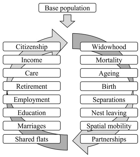
Figure 1.
Module sequence in the MikroSim model.
For this study, version 2.1.4 of the MikroSim codebase (Alsaloum et al. 2023) is used.
3.2. The Migration Module
The current migration module implemented in MikroSim can be described as an open gross migration module. In this specific approach, individuals and households immigrating (both domestic and from abroad) are created synthetically and those emigrating are deleted from the simulation. This is opposed to a closed migration approach, where domestic migration is done in a closed form, i.e., those emigrating domestically are the same units that are immigrating domestically into other districts. However, closed migration is substantially more complex and more computationally intensive. Furthermore, as opposed to the closed approach, the open one has no hard dependencies on other districts running in parallel, which makes this approach more appropriate for certain types of simulations and easier to scale for large simulation endeavors. For a more in-depth description of the implemented migration module and the selection procedure the reader is referred to Schmaus (2023).
In microsimulations, modeling migration is more challenging than in macro approaches such as the cohort component method. This is because it is essential to maintain the household structure throughout the iterations. For instance, children cannot move on their own, but only with their families. In practice, this means, that households rather than individuals need to be selected from the population to fulfill given benchmark distributions. However, obtaining household probabilities is usually not straightforward.
As a risk population for the international migration procedure, we consider all households in the population except for those living in nursing and community homes. In the first step, a pool of potentially immigrating households from abroad is constructed by duplicating existing households in the population. This cloning procedure is common in microsimulations, since creating foreign households anew is not easily done, as usually, only basic demographic information is available on international immigrants (O’Donoghue et al. 2010). This also has the advantage, that plausible combinations of individual characteristics and household structures are guaranteed. However, the cloning procedure implicitly assumes a similarity between immigrating units and already-existing units in the current population for each age-sex-citizenship-group. Heterogeneity of characteristics of the immigrating population is thus likely underestimated. For each of these newly synthesized households, the probability to immigrate is estimated via a binomial logit model. The household structure, namely the household size, presence of newborn or children aged 1 to 3 years, age of the oldest household member and marriage status, is considered in predicting the migration probability. Next, the probabilities are adjusted, such that the totals and distribution of the known benchmarks from the German migration statistics (DESTATIS 2022) are met in expectation. The distribution benchmarks indicate additional information of who is migrating, such as age, sex and citizenship (German, EU-citizen, other). A sub-function of the migration module named benchmark iterative randomized logit scaling (BIRLS) scales the households’ migration probability such that the distribution benchmarks are met as closely as possible (Schmaus 2023). Hereby, Iterative Proportional Updating (Ye et al. 2009) and Logit Scaling (Stephensen 2016) are combined to multiplicatively scale the moving probabilities for each characteristic. Iteratively, the household order is first randomized, then adjusted to match the marginal distributions, and finally rescaled until convergence is achieved. Finally, the migration process is conducted with the inverse transformation method. An equivalent procedure is repeated for the domestically immigrating population.
For the emigration procedure, we consider the entire population, including the newly immigrated households. This is because our used benchmarks list gross migration rather than net migration, i.e., households that migrated to some district and left in the same year are included in both benchmark values for immigration and emigration. The procedure is similar to immigration. However, rather than constructing a pool of potential emigrants by cloning, we consider the risk population directly. As described before, the emigration probabilities for each household are aligned towards benchmarks and scaled with the BIRLS procedure. Households which are later selected to emigrate via the inverse transformation method are simply deleted from the population entirely. Note that in a closed migration module, these households would constitute the households eligible for internal migration and would need to be allocated to other regions accordingly.
As of now, purposes of migration, such as housing, family-related issues, education, or employment (Sánchez and Andrews 2011), are not explicitly modeled but only implicitly captured by adjusting the predictions to match the specified age-sex-citizenship distributions. However, due to the calibration to the distributions, the omitted migration drivers only influence who is moving within the each age-sex-citizenship group but not the amount of people moving.
3.3. Simulation Scenarios and Assumptions
For this study, the German population was projected until the year 2050 to evaluate the impact of different migration scenarios. For this, three basic scenarios are proposed. The first one is derived as a status quo assumption and assumes a constancy of the latest observed migration numbers (Last Observed). The second scenario resembles a mean assumption on the past decade (Random). The third scenario restricts the mean assumption to years without external shocks (Restricted Random). All three scenarios are evaluated for two benchmark lengths (until 2017 and 2020). Additionally, a more sophisticated scenario is constructed, that attempts to model very recently observed migration movements for which no data is available yet (Constructed). Since only the sensitivity to migration assumptions is of interest, no further exogenous assumptions on the population development such as the life expectancy or fertility rates were implemented4. Thus, scenarios only differ regarding migration and not other demographic change components.
Since the base population is rooted in 2011, the populationwasis first projected to the current year guided by available benchmark data from official statistics on the observed levels regarding deaths, births, migration movements, marriages, education, care and employment, which are currently available on the district level up to 2020. The benchmarking procedure ensures, that the kick-off population is as close as possible to the current German population for a more realistic projection. Distributional benchmarks for migration are only available up to 2017 on the district level, however. One possibility would be to only benchmark the migration level till 2017 to not separate levels from distribution. However, this would leave out potentially influential developments for the years between 2018 to 2020, including the known migration shocks during the first year of the COVID-19 pandemic. This motivates the separate analysis for the first three scenarios for different benchmark lengths. They are once evaluated with a strict combination of migration distributions and totals (benchmark length 2017). This would imply neglecting available information on totals between 2018 and 2020. For the second set of scenarios benchmarked until 2020, distributions are artificially created according to the respective scenario (last observed value, simple mean, or restricted mean). For the latter, we opted for random samples of specified years instead of averaging, since age-sex-citizenship distributions are occasionally only available in broader classes at district level which are not comparable across the years. However, across multiple iterations, this is equal to an averaged distribution. This procedure also motivates the naming as Random and Restricted Random rather than average and restricted average.
The Last Observed and Random scenario are straightforward. Namely, they assume constant migration flows with the distribution of 2017 and the totals of 2017/2020 for the former, and the mean of the distributions from 2011–2017 and mean of the totals from 2011-2017/2011-2020 for the latter. While the Random scenario utilizes more information and is thus likely to give a more stable results than the Last Observed, it also has the notable shortcoming of including years that can be considered as special in terms of migration. This motivates the Restricted Random scenario, where such special years are left out in the averaging. Here, 2015, 2016 and 2020 cannot be sampled. The reason behind this decision is that it is known that these years are characterized by extreme migration events, namely the special migration between 2014 and 2016, which especially influenced the external migration numbers and distributions, and the COVID-19 pandemic, which has shown to be highly impactful on domestic migration. This procedure is meant to reproduce a migration pattern that can be referred to as a ’normal’ fluctuation without any special events such as economic-, health- or humanitarian crises.
Finally, the last scenario (Constructed), attempts to implement the latest migration movements, for which no data is yet available. Therefore, the already-specified Restricted Random scenario is extended by assumptions on the last two years, the current year, and short-term assumptions on the next few years. Specifically, we assume for 2021 that the migration patterns, that were also highly influenced by the ongoing COVID-19 pandemic, are very similar to 2020. Thus, the values of that year are simply repeated for 2021. For the two following years, the procedure is a bit more complex, since they are highly influenced by another transnational development, namely the Russian invasion in the Ukraine. As one can see in the years selected—2022 to 2024—the first (rather strong) assumption that has been made, is that at least the highly influential migration movements will return to ‘normal’ by the end of 2023. This is not only assumed for the immigration but also for the re-emigration mechanism. The second assumption is that concerning the totals of immigration and emigration, the migration patterns can be roughly compared to those in the years of the special migration induced by the immigration of Syrian civil-war refugees. Here we simply reuse the benchmark values of 2015 to 2017 for the years 2022 to 2024 respectively. This means that we assume very high immigration rates in the first year, followed by high emigration rates after that—either because the individuals seeking shelter in Germany move into other countries or back to their homeland. This seems true for both migration events. Additionally, first indicators hint, that both crises are very comparable regarding the total level of migration. The age, sex, and citizenship distributions, however, are known to be very different. During the years of high immigration rates of Syrian civil-war refugees, it was mainly young men from countries outside Europe who came to Germany. However, the first published figures on the recent special migration indicate that the refugee movements from Ukraine are more likely to be younger women (with children) from Europe.
To model a scenario that takes inspiration from this without the availability of reliable data on the district level, the decision to edit the distributions from 2015 to 2017 was made. For (non-German) European women the age distribution and total for 2022 to 2024 of non-European men from 2015 to 2017 were assumed. Conversely, the same period distribution and total for non-European women was assumed for European men for 2022–2024. For the non-European immigrants, the total and distributions of 2011–2013 were assumed for 2022–2024.
So as it can be seen the number of assumptions, as well as further not necessarily data-driven information that has been added, is rising in each of the scenarios, making them all more and more sophisticated and - most likely - accounting for more and more uncertainty. However, it is not necessarily the goal of this study to recommend a specific migration as the most probable one, but rather to analyze the implications of all these assumptions on a regional level and concerning several socio-demographic mechanisms.
All of the assumptions about migration totals (i.e., amount of emigration, immigration from abroad and domestically) and distribution are summarised in Table 1. The yearly migration flows (immigration, emigration and netmigration) relative to the 2020 population in the districts is shown in Figure 25. Apart from some districts in Eastern Germany, most districts are generally assumed to have a positive net migration in all scenarios due to high level of immigration to Germany. Rates for Southern and Western German districts are thereby generally higher in the sense that they have both larger flows of immigration and emigration.

Table 1.
The four migration scenarios.
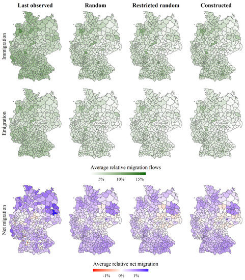
Figure 2.
Yearly migration flows relative to the 2020 population.
4. Results
For the purpose of this simulation, scenarios vary only regarding their level and age-sex-citizenship distribution. However, the microsimulation approach also allows to create migration scenarios on the unit level, for example, regarding educational level, household structures, income or other characteristics by modifying the individual characteristics of the immigrants. Additionally, various macro scenarios, such as changes in flows between rural and urban areas, could have also been implemented.
Since transitions between states are obtained by probabilistic simulation, Monte Carlo uncertainty is unavoidable. To reduce the impact of the Monte Carlo uncertainty, the arithmetic means across multiple runs per scenario are analyzed for each target variable. This is also necessary to achieve an averaging effect for the sampled years.
As previously mentioned, migration is one of the most influential factors for past and future population changes. Therefore it can be expected that changes in migration assumptions also have a rather substantial influence. Figure 3 confirms this expectation on a national level for Germany. Note, that the scenarios indiacted by the dotted (solid) lines meet the benchmarks of the population until 2017 (2020) perfectly. Population totals in 2050 vary from just over 70 Million (Last observed constant totals from 2020) to about 82 Million (Random beginning in 2017). Regardless of the chosen migration scenario, a long-term decline in the German population is projected. This long-term decline is thereby also in line with seven of the nine main variants of the official German population projection via the cohort-component method (DESTATIS 2023). However, the macro projection generally assumes a slower decline which may mainly be due to the assumed increase in life expectancy.
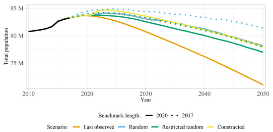
Figure 3.
Total population by migration scenario and benchmark length.
Unsurprisingly, both the beginning and the speed of the population decline differ between the assumed migration patterns in the microsimulation projection. The reasons for these differences are, however, rather obvious: Sampling out of the years from 2011 to 2017 without any restrictions implicitly assumes the possible occurrence of special migration events in the totals and distribution of 2014–2017. In contrast, freezing the rates at the level of 2020 reproduces the reduced migration movements observed during the first year of the COVID-19 pandemic for every simulated year. As expected, the random scenarios lead to the latest and slowest decline in population, while the last observed scenario with low immigration produces an immediate and fast decline.
Regarding more comparable scenarios, which means only looking at the differences between those with the same Benchmark-bases, reduces this range to 5 Million (benchmark length: 2017) or about 7.5 Million (benchmark length: 2017) respectively. Comparing the two benchmark lengths also leads to another conclusion: the scenarios in which only the years up until 2017 are considered for migration already show remarkable differences to the known population totals between 2018 and 2020. Therefore in the further analysis, only those scenarios, that start at the same point in time (2020) and take into account all available benchmarks are looked into in more detail. However, one needs to keep in mind, that while the scenarios assume the same totals of migration until 2020, they differ in the assumed distribution which is available only until 2017 regardless. Thus, for 2018 to 2020, the different scenarios are only identical regarding how many move, but not regarding who is moving.
Nevertheless, the difference of over 7.5 Million people between the two most extreme 2020 scenarios indicates, that migration scenarios and their implications shouldn’t be treated lightly already on the national level. However, so far, only external migration has been considered. Further, migration impacts are not distributed evenly across the regions. This implies, that the impacts of different migration assumptions may have severely different impacts on the sub-national level with some districts on ’the winning end’ of migration while others may face a stark decline in population.
Huge differences in the regional development of population totals for the 401 German districts between 2020 and 2050 are immediately identifiable. While some districts are facing a decline in population, other districts remain largely unchanged or experience further growth in population. On average, we project a population decline in the districts between 10.2% (Random) and 14.8% (Last Observed). Notably, some smaller districts, for example Frankfurt (Oder) with less than 60,000 inhabitants in 2020, are projected to see a very large decline in population in the Last Observed scenario but not in others. The largest projected growth is for the district Cloppenburg with a projected growth of around 30%, again in the Last Observed scenario. Such extreme developments are due to the reliance on a single year migration total for the Last Observed scenario and are not visible in the other scenarios. For instance, the district Stadtkreis Heidelberg is projected to see a decline in population of over 70% in the Last Observed scenario but is projected a growing population of 3 to 8% in the other scenarios. Similarly, Cloppenburg is only projected to grow by 13 to 16% in the other scenarios. The projected changes are shown in Figure 4. Note, however, that the percentage changes have been truncated to ease interpretation. Generally, it can be observed that under the specified scenarios, more rural areas such as most eastern German districts and districts in middle Germany, Rhineland-Palatinate or Saarland are expected to see a decline in population size till 2050. In contrast, urbanized districts, such as the city districts of Berlin, Hamburg or Munich, as well as southern Germany tend to see an increase in population size.
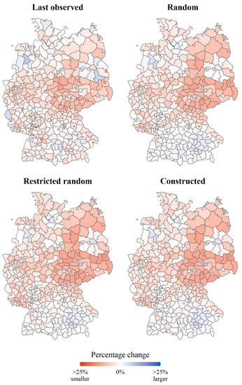
Figure 4.
Relative change in population 2020 to 2050.
Comparing the results between the scenarios, one can observe visible differences of Last Observed to the other migration scenarios. Some districts that are projected to see an increase in population in the Last Observed scenario are projected to see a decline in population in the three other scenarios. While especially big cities such as the aforementioned Berlin, Hamburg or Munich are shrinking only in this scenario, other rural areas, most of them around these big cities, seem to profit from this development. So assuming the trend that seems to have started during the COVID-19 pandemic—regardless if it was triggered by housing prices, changes in employment structures or other socio-demographic mechanisms—would in our model not change the development in Germany in general, but would lead to a lower concentration of people in the biggest city, since they seem to move to the suburban areas. The effect of 2020 as a special year for internal migration can also be seen in the Random scenario compared to the other two scenarios where the migration rates of 2020 are of no further importance in the future. Here it also seems that the German population is at least a bit more distributed between urban and rural areas. Unsurprisingly, the Constructed scenario barely differs from the Restricted Random scenario in the long run. While the increased immigration for 2022 due to recent events was considered, this has barely an effect in 2050, since an increased emigration was assumed for the after-years. After 2024, this scenario is also equivalent to the Restricted Random scenario both in total and distributions such that no stark differences were expected.
The distribution of percentage changes in population of 2050 compared to 2020 is shown in Figure 5. It becomes visible, that the Last Observed scenario produces both the most extreme growths and declines of all scenarios. Additionally, it generally produces the greatest decline in population for all the districts.
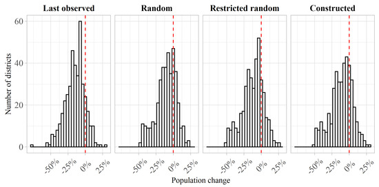
Figure 5.
Distribution of relative changes in population 2020 to 2050.
Apart from the size of the population, the structure is usually of interest for policy planning. One important indicator is the Old Age Dependency Ratio (OADR), which relates the number of elder persons to the number of people of working age. Here, following the calculation of the indicator by the German Statistical Office, we defined the potential working population as people aged 15 to 64, and the people above working age as 65 or older accordingly. This indicator is of particular interest since the demographic change is assumed to have a huge impact on German society. The OADR can be seen as a proxy indicator for several social and economic challenges that Germany has to face in the future, namely for example questions about employment, pensions, care or medical care structures. The results are presented in Figure 6. For the further analysis the specified scenarios are compared to the Random scenario which we considered a good baseline scenario, as mean assumptions on migration are relatively common in practice.
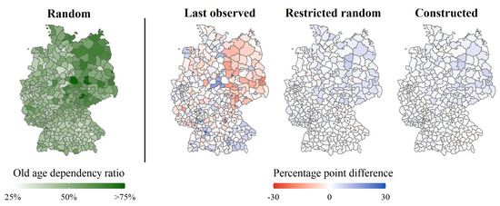
Figure 6.
Difference to the ’random’ scenario in the 2050 old age dependency ratio.
The OADR is generally increasing in our simulations, by more than ten percentage points until 2050. This development is expected due to the known demographic change in Germany. The development is primarily a result of the underlying demographic structure of the population and is unlikely to be reversed even by a continuous and high level of immigration by young people. However, the development of the OADR is not of primary interest but rather the differences in development between the migration scenarios. Even repeating special migration scenarios such as the one between 2014 and 2017, which are assumed in the Random scenario, are not able to lead to a remarkably different demographic structure in Germany. Nevertheless, regional differences in the level of old age dependency are visible in Figure 6 for the Random scenario. Especially districts in eastern Germany are hit by these developments and in 2050 have the highest OADRs—which itself is again a rather common assumption on the future development of age distributions in Germany. However, a different development can be seen in the other migration scenarios: Compared to the Random scenario both, the Restricted random and the Constructed scenario, show a stronger increase in old age dependency across most of the districts in Germany. Assuming a more regular immigration without sudden and strong inflows of young people would lead to an even stronger increase in the OADR. Moreover, the implications of the Constructed scenario don’t seem to have a visible difference to the Restricted random one, although here another special migration event has been implemented. However, this one-time special migration event doesn’t seem to have a sustaining impact on the demographic structure. This is also due to the fact, that higher emigration rates were assumed for the years 2023 and 2024, assuming. Regarding the regional differences, the two aforementioned scenarios don’t show any systematic differences from one another or the comparison scenario. The former is again unsurprising since the same migration structure was assumed after 2024 for both scenarios.
This is different for the Last observed scenario. Here it can be seen again, that leaving the year 2020 with its impact on internal migration in Germany constant, leads to kind of a redistribution between densely populated urban areas and the thinly populated districts around them. While urban areas, in general, have rather low OADRs compared to rural ones, their numbers are rising by about 30 percentage points, whereas these numbers are reversed in rural districts, especially in eastern Germany. So under the assumption that the migration patterns that could be observed during 2020 are the indicator for a change in trend—perhaps due to changes in working conditions or constantly rising housing prices- rather than a special migration event, equalization in the OADRs in Germany can be expected.
Microsimulation also allows the exploration of additional demographic and non-demographic by-effects of implemented what-if scenarios. One of the by-effects of structural changes in the employment market, which is modeled in dependency of individual socio-demographic characteristics, education and household structure in MikroSim. For the further analysis, the participation rate on the district level is considered. It relates the number of people aged 15 to 64 in work to the total number of people aged 15 to 64. This relative number is especially interesting because the effects of migration are showing beyond the sheer quantity of migration (which also affects the absolute number of working people) and is influenced by many factors such as sex distribution or even citizenship itself. The level of the participation rate and the percentage point difference of the scenarios to the Random scenario is shown in Figure 7. It can be seen, that the projected participation rates for 2050 differ strongly within Germany with a range of 25 percentage points between the districts. Especially in southern Germany, participation rates are higher than in the north and east. However, the pattern is less clear than for the OADRs. Although rural areas all over Germany seem to have fewer people between 15 and 65 years of age working, districts in the south of Germany, some of which are thinly populated, have some of the highest participation rates. In addition, some urban areas such as Berlin also show rather low participation rates.
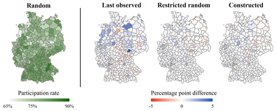
Figure 7.
Difference to the ’random’ scenario in the 2050 participation rate.
While there is hardly any variability between the scenarios on a national level, differences of up to 5 percentage points between the scenarios become visible at the district level. One possible explanation are again differences in the age, sex and citizenship distributions. It is known and can be seen in almost all available empirical data, that men are more likely to be employed, mostly because women are more likely to do unpaid work such as childcare or caring for relatives. However, the differences between the scenarios are relatively small apart from the Last Observed which would result in a slightly higher participation rate. For the vast majority of district, this difference is well below one percentage point. Further, a clear regional pattern in the differences is not directly observable. Unlike for the OADR, a clear overall tendency is also not visible for the Restricted random and Constructed scenarios. For both scenarios, the OADR was higher in most districts than in the Random scenario. Looking at the specific participation rates, however, some districts benefit from (slightly) higher participation rates while others face a reduced share of people in work.
Figure 8 shows a categorization of the districts in Germany into four settlement structure types following the classification of the BBSR (Bundesinstitut für Bau-, Stadt, und Raumforschung 2020). This classifies the German districts into four types: large cities, urban districts, rural districts, and thinly populated rural districts. This frame opens up another possible level for analyzing the simulated data. The development of the participation rate and OADR by district type throughout the simulated time is shown in Figure 9. This classification thereby emphasizes the findings discussed above: Especially large cities are highly influenced by a Last observed scenario regarding the OADR, mainly because here the effects of the COVID-19 pandemic are assumed to remain constant in the future. In addition, this perspective leads to another interesting conclusion, namely that the rise of the OADRs becomes steeper with a shrinking population density - almost regardless of the implemented migration scenario. However, analyzing the development of the participation rates for the different settlement structure types, no remarkable difference for the scenarios is observable. This also underlines the precious conclusion that there are no visible patterns in the distribution of changes in participation rates between migration scenarios. Nevertheless, this points to the conclusion that more research on explanatory factors for the in part, strongly diverging effects of the different assumptions on future migration movements in some districts is needed.
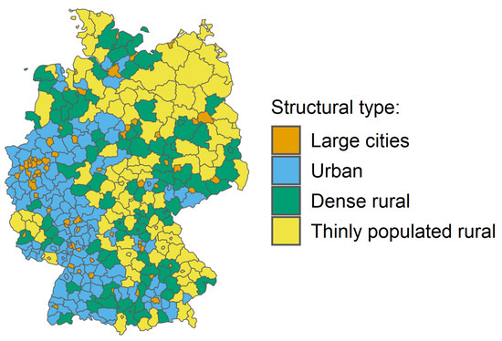
Figure 8.
German districts by settlement structural type.
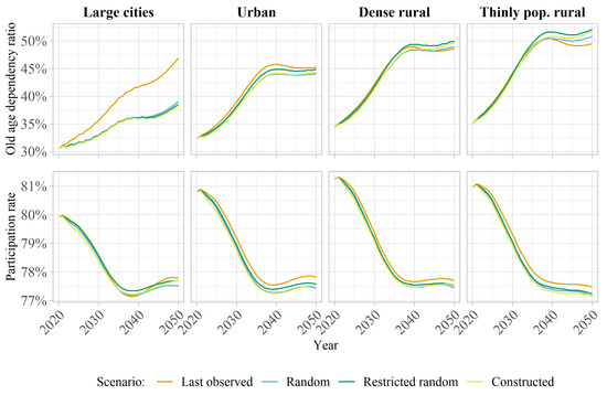
Figure 9.
Development of the participation rate and old age dependency ratio by structural type.
5. Discussion and Conclusions
Assumptions on future migration are of crucial importance for any population projection, especially, when regionalized projections are of interest. One strength of the microsimulation approach is the joint projection of many interacting individual characteristics in the population. However, since the variables are strongly interacting with each other, this also means, that indicators could potentially react very strongly to changes in seemingly not or only hardly related characteristics. In this paper, the sensitivity of total population, the old age dependency ratio, and participation rate to different assumptions on migration totals and distributions were analyzed in a microsimulation context. While other non-demographic events such as the generation of income, care, education trajectories or partnership formation are also modeled in MikroSim, an extensive analysis of all indicators was not possible in this study. The microsimulation approach would also allow for the construction of scenarios on the micro level such as changes in individual traits of the immigrants. However, for the sake of this study, only totals and distributions were altered between the scenarios.
We find that the specification of future migration totals and distributions influenced all analyzed indicators, however, to a very different degree. While projected population changes reacted very strongly to differences in assumptions, participation rates were influenced way less strongly. The differences between the scenarios thereby increase with time. Analyzing the impact on a regional level also highlights the heterogeneity of the effects of migration assumptions. Here, different scenarios can lead to extreme changes in districts. Some trends projected in one scenario where thereby even reversed in other scenarios. Interestingly, not only very small districts but also larger cities are affected by this.
Finding a reasonable future migration scenario is no straightforward task since future flows of immigration and emigration are the result of a complex interaction between political and economical factors. Ultimately, only the future can tell how well a scenario has been specified. However, at least in terms of plausibility and stability, some conclusions may still be drawn from this study. For example, the relatively naive status quo assumption, meaning that the year 2020 would repeat every following year, seems highly improbable. Moreover, this has a high risk to ignore known and relatively stable migration trends in individual districts, since one-time events solely decide about future development. Regarding the other scenarios, the results in the simulation are at least somewhat comparable. Only on the district level and taking age and sex distributions into account some influences can be seen. Conversely, a scenario such as the Constructed scenario with a high number of assumptions about the near future of migration patterns that aren’t necessarily grounded in actual empirical data, can perform quite well at least in terms of stability and plausibility. So, without any other evidence, it seems to always be good advice to implement additional information—either validated empirically or by experts in this field—into assumptions about future migration patterns.
However, several shortcomings of this study should be mentioned. A central driver of internal migration that should be further analyzed is the housing market. Especially in large city districts, capacities for the creation of additional living space are already very limited. The continuation of growth from the past is highly unlikely for already densely populated districts. Conversely, thinly populated districts may become more attractive in the future due to lower rent prices and lacking living opportunities in densely populated districts. Future migration allocation will be strongly connected to the affordability of housing. As of now, the housing market is not implemented yet in MikroSim, however, this is planned for the future. Economic factors such as labour market opportunities or regional wage differentials are also crucial in understanding future migration development (Bijak 2006; Brunow et al. 2015) but have been neglected in this simulation. Further future research potential lies in the exploration of migration scenarios in a closed migration setting. This would allow for the implementation of more realistic emigration modeling, namely, having the outmigration depend on the current population size. In open migration, this is not straightforward for consistency reasons. Here, we would expect less extreme developments. On one side, larger districts would experience a stronger emigration with increasing population size, while shrinking districts would see a decreasing outmigration with a reduction of the risk population. Finally, this approach also allows to fully utilize migration trajectories as predictors. This may also prove very useful in modeling who is moving, since past migration tends to be a strong predictor for future migration.
Author Contributions
Conceptualization, J.E., S.D., S.S., J.W., A.A. and R.M.; methodology, J.E., S.D., S.S., J.W. and A.A.; software, J.E., S.D., S.S., J.W. and A.A.; validation, J.E., S.D., J.W., A.A.; formal analysis, J.E., S.D., J.W. and A.A.; investigation, J.E., S.D., S.S., J.W. and A.A.; resources, R.M.; data curation, J.E., S.D., S.S., J.W. and A.A.; writing—original draft preparation, J.E., S.D., S.S., J.W. and A.A.; writing—review and editing, J.E., S.S., R.M.; visualization, J.E.; supervision, R.M.; project administration, R.M.; funding acquisition, R.M. All authors have read and agreed to the published version of the manuscript.
Funding
This research was funded by the German Research Foundation (DFG) grant number FOR 2559.
Institutional Review Board Statement
Not applicable.
Informed Consent Statement
Not applicable.
Data Availability Statement
As of now, the data are subject to disclosure control. However, the data are expected to be submitted to a research data lab within the MikroSim project.
Acknowledgments
The research was conducted as part of the Research Unit FOR 2559 MikroSim.
Conflicts of Interest
The authors declare no conflict of interest.
Notes
| 1 | In fact, this methodological agenda almost entirely lost its significance for the social sciences after a peak in Germany in the 1990s in the context of the research efforts of the well-known special research unit 3 (Hauser et al. 1994), where some of the most sophisticated microsimulation models up to that point have been developed. |
| 2 | While the calibration of the models to known regional totals allows a regionalization of the models, structural differences that are not introduced by individual differences may still be underestimated. Ideally, models would be estimated for each region separately, however, this is not feasible in practice due to limitations in sample size for each district. |
| 3 | Note that before 2015, Germany was separated into 402 districts. |
| 4 | Note, however, that the status quo assumption is only on the coefficients of the mortality and fertility models. Thus, changes in observed rates for fertility and life expectancy are only due to changes in the individual characteristics. For instance, increasing education levels in the population or reduction of partnerships and marriages will decrease the overall birth probabilities. |
| 5 | In the simulation itself, migration flows are not modeled relative to population size but as totals. However, for the purpose of visualization, interpretation of flows becomes more straightforward when related to the population sizes, since the larger districts naturally have higher total in immi- and emigration. |
References
- Ahn, Namkee, Juha M Ahlo, Herbert Brücker, Harri Cruijsen, Seppo Laakso, Jukka Lassila, and Tarmo Valkonen. 2013. The Use of Demographic Trends and Long-Term Population Projections in Public Policy Planning at EU, National, Regional and Local Level: Summary, Conclusions and Recommendations. Brussels: European Union: Lot 1 Study Group. [Google Scholar]
- Alsaloum, Ahmed, Hanna Dieckmann, Sebastian Dräger, Jana Emmenegger, Julian Ernst, Florian Ertz, Philip Höcker, Hariolf Merkle, Jannek Mülhan, Kristina Neufang, and et al. 2023. MikroSim Codebase. Version 2.1.4 (Internal Release). Trier, Wiesbaden, Duisburg and Berlin: MikroSim. [Google Scholar]
- Bae, Jang Won, Euihyun Paik, Kiho Kim, Karandeep Singh, and Mazhar Sajjad. 2016. Combining microsimulation and agent-based model for micro-level population dynamics. Procedia Computer Science 80: 507–17. [Google Scholar] [CrossRef]
- Ballas, Dimitris, Tom Broomhead, and Phil Mike Jones. 2019. Spatial Microsimulation and Agent-Based Modelling. Cham: Springer International Publishing, pp. 69–84. [Google Scholar] [CrossRef]
- Bijak, Jakub. 2006. Forecasting International Migration: Selected Theories, Models, and Methods. Warsaw: Central European Forum for Migration Research. [Google Scholar]
- Bijak, Jakub. 2011. Explaining Migration: Brief Overview of Selected Theories. Dordrecht: Springer, pp. 37–51. [Google Scholar]
- Bijak, Jakub, and Mathias Czaika. 2020. Black swans and grey rhinos: Migration policy under uncertainty. Migration Policy Practice X 4: 14–20. [Google Scholar]
- Brunow, Stephan, Peter Nijkamp, and Jacques Poot. 2015. The impact of international migration on economic growth in the global economy. In Handbook of the Economics of International Migration. Amsterdam: Elsevier, vol. 1, pp. 1027–75. [Google Scholar]
- Bundesinstitut für Bau-, Stadt, und Raumforschung. 2020. Archiv Raumbegrenzungen. Available online: https://www.bbsr.bund.de/BBSR/DE/forschung/raumbeobachtung/downloads/archiv/download-referenzen.html (accessed on 19 February 2023).
- Burch, Thomas K. 2018. Model-Based Demography: Essays on Integrating Data, Technique and Theory. Berlin and Heidelberg: Springer Nature. [Google Scholar]
- Burgard, Jan Pablo, Hanna Dieckmann, Joscha Krause, Hariolf Merkle, R. Münnich, Kristina M Neufang, and Simon Schmaus. 2020. A generic business process model for conducting microsimulation studies. Statistics in Transition New Series 21: 191–211. [Google Scholar] [CrossRef]
- Burgard, Jan Pablo, Joscha Krause, Hariolf Merkle, Ralf Münnich, and Simon Schmaus. 2020. Dynamische Mikrosimulationen zur Analyse und Planung regionaler Versorgungsstrukturen in der Pflege. In Mikrosimulationen. Wiesbaden: Springer, pp. 283–313. [Google Scholar]
- Burgard, Jan Pablo, Joscha Krause, and Simon Schmaus. 2021. Estimation of regional transition probabilities for spatial dynamic microsimulations from survey data lacking in regional detail. Computational Statistics & Data Analysis 154: 107048. [Google Scholar]
- Caswell, Hal, and Nora Sánchez Gassen. 2015. The sensitivity analysis of population projections. Demographic Research 33: 801–40. [Google Scholar] [CrossRef]
- Clark, Stephen, Mark Birkin, Alison Heppenstall, and Philip Rees. 2017. Using 2011 census data to estimate future elderly health care demand. In The Routledge Handbook of Census Resources, Methods and Applications. Abingdon: Routledge, pp. 305–19. [Google Scholar]
- DESTATIS. 2019. Bevölkerung im Wandel. Annahmen und Ergebnisse der 14. koordinierten Bevölkerungsvorausberechnung. Technical Report. Available online: https://www.destatis.de/DE/Presse/Pressekonferenzen/2019/Bevoelkerung/bevoelkerung-uebersicht.html (accessed on 15 December 2022).
- DESTATIS. 2022. Bevölkerung und Erwerbstätigkeit: Wanderungen. Fachserie 1 Reihe 1.2. Available online: https://www.destatis.de/DE/Themen/Gesellschaft-Umwelt/Bevoelkerung/Wanderungen/Publikationen/Downloads-Wanderungen/wanderungen-2010120217004.pdf (accessed on 15 January 2022).
- DESTATIS. 2023. 15. koordinierte Bevölkerungsvorausberechnung. Available online: https://www.destatis.de/DE/Themen/Gesellschaft-Umwelt/Bevoelkerung/Bevoelkerungsvorausberechnung/begleitheft.html (accessed on 27 February 2023).
- Galler, Heinz P. 1997. Discrete-Time and Continous-Time Approaches to Dynamic Microsimulation Reconsidered. Canberra: National Centre for Social and Economic Modelling. [Google Scholar]
- Hannappel, Marc, and Klaus G. Troitzsch. 2015. Mikrosimulationsmodelle. In Handbuch Modellbildung und Simulation in den Sozialwissenschaften. Edited by Norman Braun and Nicole J. Saam. Wiesbaden: Springer Science and Business Media, pp. 455–90. [Google Scholar]
- Hansen, Jonas Zangenberg, Peter Stephensen, and Joachim Borg Kristensen. 2013. Modeling household formation and housing demand in denmark. In DREAM, Danish Rational Economic Agents Model. Copenhagen: Statistics Denmark, pp. 115–22. [Google Scholar]
- Hauser, Richard, Notburga Ott, and Gerd Wagner. 1994. Mikroanalytische Grundlagen der Gesellschaftspolitik. Band 2: Erhebungsverfahren, Analysemethoden und Mikrosimulation. Ergebnisse aus dem gleichnamigen Sonderforschungsbereich an den Universitäten Frankfurt und Mannheim. Berlin: Wiley-VCH Verlag GmbH. [Google Scholar]
- Howe, Neil, and Richard Jackson. 2004. Projecting Immigration: A Survey of the Current State of Practice and Theory. Technical Report. Available online: https://www.csis.org/analysis/projecting-immigration (accessed on 15 December 2022).
- Jahn, Beate, Sarah Friedrich, Joachim Behnke, Joachim Engel, Ursula Garczarek, Ralf Münnich, Markus Pauly, Adalbert Wilhelm, Olaf Wolkenhauer, Markus Zwick, and et al. 2022. On the role of data, statistics and decisions in a pandemic. AStA Advances in Statistical Analysis 106: 349–82. [Google Scholar] [CrossRef]
- Keyfitz, Nathan. 1972. On future population. Journal of the American Statistical Association 67: 347–63. [Google Scholar] [CrossRef] [PubMed]
- Lee, Everett S. 1966. A theory of migration. Demography 3: 47–57. [Google Scholar] [CrossRef]
- Li, Jinjing. 2014. Dynamic models. In Handbook of Microsimulation Modelling. Edited by Cathal O’Donoghue. Bingley: Emerald Publishing Limited, pp. 305–43. [Google Scholar]
- Li, Jinjing, and Cathal O’Donoghue. 2013. A survey of dynamic microsimulation models: Uses, model structure and methodology. International Journal of Microsimulation 6: 3–55. [Google Scholar] [CrossRef]
- Lovelace, Robin, and Morgane Dumont. 2017. Spatial Microsimulation with R. Boca Raton: Chapman and Hall/CRC. [Google Scholar]
- Marois, Guillaume, and Arda Aktas. 2021. Projecting health-ageing trajectories in europe using a dynamic microsimulation model. Scientific Reports 11: 1785. [Google Scholar] [CrossRef]
- Marois, Guillaume, and Samir KC. 2021. Microsimulation Population Projections with SAS: A Reference Guide. Cham: Springer Nature. [Google Scholar]
- Münnich, Ralf, Rainer Schnell, Johannes Kopp, Petra Stein, Markus Zwick, Sebastian Dräger, Hariolf Merkle, Monika Obersneider, Nico Richter, and Simon Schmaus. 2020. Zur Entwicklung eines kleinräumigen und sektorenübergreifenden Mikrosimulationsmodells für Deutschland. Wiesbaden: Springer Fachmedien Wiesbaden, pp. 109–38. [Google Scholar] [CrossRef]
- O’Donoghue, Cathal, Howard Redway, and John Lennon. 2010. Simulating migration in the pensim2 dynamic microsimulation model. International Journal of Microsimulation 3: 65–79. [Google Scholar] [CrossRef]
- O’Neill, Brian C, Deborah Balk, Melanie Brickman, and Markos Ezra. 2001. A guide to global population projections. Demographic Research 4: 203–88. [Google Scholar] [CrossRef]
- Orcutt, Guy H. 1957. A new type of socio-economic system. The Review of Economics and Statistics 39: 116–23. [Google Scholar] [CrossRef]
- Preston, Samuel, Patrick Heuveline, and Michael Guillot. 2000. Demography: Measuring and Modeling Population Processes. Malden, MA: Blackwell Publishers. [Google Scholar]
- Sánchez, Aida Caldera, and Dan Andrews. 2011. To Move or Not to Move: What Drives Residential Mobility Rates in the OECD? Available online: https://doi.org/10.1787/5kghtc7kzx21-en (accessed on 15 January 2023).
- Schmaus, Simon. 2023. Methoden dynamischer regionalisierter Mikrosimulationen. Ph.D. thesis, Universität Trier, Trier, Germany. [Google Scholar]
- Smith, Stanley K., Jeff Tayman, and David A. Swanson. 2013. A Practitioner’s Guide to State and Local Population Projections. Dordrecht: Springer. [Google Scholar]
- Spielauer, Martin. 2009. Microsimulation Approaches. Statistics Canada Working Paper. Available online: https://www.statcan.gc.ca/en/microsimulation/modgen/new/chap2/chap2 (accessed on 15 December 2022).
- Spielauer, Martin. 2011. What is social science microsimulation? Social Science Computer Review 29: 9–20. [Google Scholar] [CrossRef]
- Stephensen, Peter. 2016. Logit scaling: A general method for alignment in microsimulation models. International Journal of Microsimulation 9: 89–102. [Google Scholar] [CrossRef]
- Thomas, Jason R., and Samuel J. Clark. 2011. More on the cohort-component model of population projection in the context of hiv/aids: A leslie matrix representation and new estimates. Demographic Research 25: 39. [Google Scholar] [CrossRef]
- Van Imhoff, Evert, and Wendy Post. 1998. Microsimulation methods for population projection. Population: An English Selection 10: 97–138. [Google Scholar]
- Wilson, Tom. 2022. Preparing local area population forecasts using a bi-regional cohort-component model without the need for local migration data. Demographic Research 46: 919–56. [Google Scholar] [CrossRef]
- Wilson, Tom, and Martin Bell. 2004. Comparative empirical evaluations of internal migration models in subnational population projections. Journal of Population Research 21: 127–60. [Google Scholar] [CrossRef]
- Wilson, Tom, Irina Grossman, Monica Alexander, Phil Rees, and Jeromey Temple. 2022. Methods for small area population forecasts: State-of-the-art and research needs. Population Research and Policy Review 41: 865–98. [Google Scholar] [CrossRef]
- Wilson, Tom, and Phil Rees. 2005. Recent developments in population projection methodology: A review. Population, Space and Place 11: 337–60. [Google Scholar] [CrossRef]
- Wittenberg, Raphael, Ruth Hancock, Adelina Comas-Herrera, Derek King, Juliette Malley, Linda Pickard, Ariadna Juarez-Garcia, and Robin Darton. 2007. Model 11: PSSRU long-term care finance model and CARESIM: Two linked UK models of long-term care for older people. In Modelling Our Future: Population Ageing, Health and Aged Care. Bingleyl: Emerald Group Publishing Limited. [Google Scholar]
- Ye, Xin, Karthik Konduri, Ram M. Pendyala, Bhargava Sana, and Paul Waddell. 2009. A methodology to match distributions of both household and person attributes in the generation of synthetic populations. Paper presented at the 88th Annual Meeting of the Transportation Research Board, Washington, DC, USA, January 11–15. [Google Scholar]
- Zika, Gerd, Markus Hummel, Marc Ingo Wolter, and Tobias Maier. 2023. Das QuBe-Projekt: Modelle, Module, Methoden. Bielefeld: DE wbv Media. [Google Scholar]
- Zwick, Markus, and Jana Emmenegger. 2020. Mikrosimulation und Gesellschaftspolitik-ein kurzer historischer Abriss. In Mikrosimulationen. Edited by Marc Hannappel and Johannes Kopp. Wiesbaden: Springer VS, pp. 17–34. [Google Scholar]


Disclaimer/Publisher’s Note: The statements, opinions and data contained in all publications are solely those of the individual author(s) and contributor(s) and not of MDPI and/or the editor(s). MDPI and/or the editor(s) disclaim responsibility for any injury to people or property resulting from any ideas, methods, instructions or products referred to in the content. |
© 2023 by the authors. Licensee MDPI, Basel, Switzerland. This article is an open access article distributed under the terms and conditions of the Creative Commons Attribution (CC BY) license (https://creativecommons.org/licenses/by/4.0/).