Article

A Non-Linear Continuous-Time Generalized Predictive Control for a Planar Cable-Driven Parallel Robot

1
Department of Mechanical Engineering, Automatic Laboratory, University of Skikda, 21000 Skikda, Algeria
2
DIMEG, Univesity of Calabria, Via Bucci Cubo 45C, 87036 Rende, Italy
*
Authors to whom correspondence should be addressed.
Actuators 2021, 10(5), 97; https://doi.org/10.3390/act10050097
Submission received: 13 February 2021 / Revised: 29 April 2021 / Accepted: 30 April 2021 / Published: 4 May 2021
(This article belongs to the Special Issue Advanced Robots: Design, Control and Application)

Abstract

:
This paper addresses a novel nonlinear algorithm for the trajectory tracking of a planar cable-driven parallel robot. In particular, we outline a nonlinear continuous-time generalized predictive control (NCGPC). The proposed controller design is based on the finite horizon continuous-time minimization of a quadratic predicted cost function. The tracking error in the receding horizon is approximated using a Taylor-series expansion. The main advantage of the proposed NCGPC is based on using an analytic solution, which can be truncated to a desired degree of order of the Taylor-series. This allows us to achieve a prediction horizon of NCGPC tracking performance. The description of the proposed NCGPC method is followed by a comparison between NCGPC and a conventional computed torque control (CTC) method. Robustness tests are performed by considering payload and parameter uncertainties for both controllers. Simulation results of NCGPC compared to the commonly used CTC prove the effectiveness and advantages of the proposed approach.

1. Introduction

Cable-driven parallel robots (CDPRs) are a class of parallel robots where the end-effector is supported by a system of cables, which are extended or retracted by using motors and pulleys. Recently, CDPRs are widely used for several applications, such as lifting heavy loads and rehabilitation applications, as reported, for example, by Albus et al. [1], Tang [2], Pinto et al. [3], and Morizono et al. [4]. The challenges arising in the control of CDPRs have been the subject of many research works. Particularly significant in this field are, for example, the work on orientability by Vikranth Reddy [5]; the work [6] where the control takes into account the viscoelastic effect of cables; the work on the pseudo-drag effect at high speed that is reported, for example, in [7]; or the work on high-frequency and oscillation reduction that is reported, for example, in [8].
The accuracy of a cable-driven parallel robot can be strongly affected by the implemented control strategy. In this paper, we propose a robust control strategy for the real-time control of a cable-driven robot. In recent decades, predictive control has become one of the most important research topics in nonlinear control systems, such as that reported by Koreyam et al. for ICaSbot CDPR in [9], or by considerations on the feasibility for enhanced control strategies, as reported in [10]. Model predictive control (MPC), also known as receding horizon control, is generally based on a priori knowledge of the process via a prediction model ensuring the estimation of the future outputs. This can be achieved by means of frequency analyses, as proposed, for example, in [11], or by establishing proper dynamic models with cable elasticity, as reported, for example, in [12]. Once this model has been determined, the MPC algorithm can be formulated as an online optimization problem on a finite moving horizon. At each sampling step, the controller tries to minimize the cost functions subject to specific constraints. Constraints can be set on the feedback linearization, as proposed, for example, in [13]; they can be based on adaptative control strategies, as proposed, for example, in [14]; or they can be defined on elastic models of the actuators, as proposed, for example, in [15]. When the control sequence is found, only the first component is applied to the process. At the next sampling time, the prediction horizon moves one step forward, and the optimization problem is repeated iteratively. However, the above-mentioned problem becomes more difficult, or even impossible to solve, when it is implemented for nonlinear systems with fast dynamics, especially in the case where several constraints are considered, such as that proposed by Inel et al. in [16] or by Carbone et al. in [17]. This is because the on-line nonlinear optimization algorithm imposes a heavy computational burden which requires a large computation time, as reported, for example, by Tang and Shao in [18], by Li et al. in [19], or by Poignet and Gautier in [20]. Therefore, in most cases, linear models are used to predict the future behavior of the nonlinear system over a finite horizon. The advantage of using linearized prediction models lies in the fact that in the absence of constraints, the optimal solution can be written explicitly. Nevertheless, the robustness of the control law depends directly on considering the nonlinear nature of the system. Nonlinear model predictive control (NMPC) is, therefore, a powerful strategy. The best way to address these difficulties arising in the design and implantation of NMPC is to adopt an analytic approach, where the control problem is formulated in a closed form to avoid online optimization with the approach proposed, for example, in [21] or the application proposed by Hedjar et al. in [22].
Non-linear continuous-time generalized predictive control (NCGPC) was first proposed in [23] for linear plants. It has similar properties to those of the discrete time generalized predictive control (GPC), and it is a promising alternative for dealing with fast dynamic nonlinear systems, as mentioned, for example, in [24]. In general, the predictive control problem has specific advantages for solving—in real time—a finite horizon closed-loop optimal control subject to the system dynamic constraints involving states and controls. The main advantage of MPC is the fact that it allows the current timeslot to be optimized while taking future timeslots into account. This is achieved by optimizing a finite time horizon while only implementing the current timeslot and then optimizing again for the next timeslot.
The NCGPC prediction model is based on Taylor series expansion. However, obtaining an analytic solution imposes a constraint on the order of the Taylor-series expansion to the corresponding output relative degree [25,26]. Most work in generalized predictive control is based on a discrete-time approach, but one can use a transfer function approach to achieve a continuous-time approach. Note that this control strategy requires the stability of all zero dynamics, and the closed-loop system stability is guaranteed for a relative degree less than or equal to four.
The aim of this work is the application and implementation of an NCGPC control algorithm for the motion control of a planar four-cable-driven parallel robot. The proposed control strategy is based on a generalized predictive control with a discrete-time approach, including dynamic constraints. The predictive error is obtained in advance by expanding the output and reference signals in an ri-th order Taylor series, where ri is the relative degree of the i-th output (relative degree ri ≤ 4, where ri is the number of motors). Accordingly, the Taylor series is set to be lower than the number of active motors, as proposed, for example, in [27]. This proposed approach is implemented for a specific case study and compared with a conventional control approach. The obtained results demonstrate the engineering feasibility, robustness, and enhanced performance of the proposed approach. Note that four active motors are defined in the case of the study that is addressed in this paper. However, the proposed approach can be generalized to any CDPR.
The paper is organized into six sections. Section 2 is dedicated to the proposed robot modeling required for the control strategy design. Section 3 presents the control problem formulation and the corresponding solution. Then, the stability analysis is discussed in the following section. In Section 5, simulation results are presented. Finally, conclusions are given.

2. Robot Structure and Modeling

This paper focuses at a two-degree of freedom (DOF) planar cable-driven parallel robot, whose kinematic scheme and main geometric parameters are reported in Figure 1. This specific design was introduced in [28]. It is suitable for multiple applications, from conventional pick and place tasks to rehabilitation exercises of human upper limbs. This case study was selected since its dynamics are well known. However, the proposed control approach can be generalized, and it can be conveniently applied, for example, to spatial cable-driven robots.
The main geometric parameters of the robot are described in Table 1 by referring to the schemes in Figure 1.
The dynamics of the platform are given by the following equation:
  M e q ( X ) X ¨ + N ( X , X ˙ ) = F V
where the bold type indicates a matrix or vector; X ¨ is the inertial matrix; N ( X , X ˙ ) is the matrix of Coriolis that can be written as
M e q ( X ) = r m + S ( X )   J   β x ;   N ( X , X ˙ ) = S ( X ) ( J   d dt ( β x ) + C   β x ) X ˙
where r is the matrix of the pulley radiuses ri = r and
m = [ m 0 0 m ] ;   J = [ J 1 0 0 J 4 ] ;   C = [ c 1 0 0 c 4 ] ;   X = [ x m y m ] T
where the T apex represents the transpose operator.
The virtual Cartesian force input F V is defined as
F V = S ( X )   τ
The pulley angle vector can be written as a function of driven cable lengths as
β = [ β 1 ( X ) β 4 ( X ) ] = 1 r [ L 01 ( x m A 1 x ) 2 + ( y m A 1 y ) 2 L 04 ( x m A 4 x ) 2 + ( y m A 4 y ) 2 ]
The Jacobian matrix S ( X ) is given by
S ( X ) = [ cos θ 1 cos θ 4 sin θ 1 sin θ 4 ]
where
θ i = atan 1 ( x m A ix y m A iy )
where i = 1, …, 4.
Choosing x = [ x 1 x 2 ] T = [ X T X ˙ T ] T as state vector and U = F V   as the control input, the proposed robot dynamic model given by Equation (1) can be rewritten in the form of
{ X ˙ 1 = x 2   x ˙ 2 = f ( x ) + g ( x ) U   y = h ( x ) = x 1  
where
f ( x ) = N ( x ) ;   g ( x ) = M e q 1 ( x )

3. The Proposed NCGCP Controller Design

One can consider the following multiple input–multiple output (MIMO) nonlinear system, whose nomenclature of parameters variables is shown in Table 2.
{ x ˙ = F ( x ) + i = 1 m g i ( x ) u i = F ( x ) + G ( x )   U     y = h ( x ) = [ h 1 ( x ) , h 2 ( x ) , , h m ( x ) ] T
where x ∈ Rn, U ∈ Rm and y ∈ Rm are, respectively, the state vector, the control vector and the output vector. F(x) and h(x) are smooth vector fields.
As in the nonlinear case, the predictive control is based in taking the derivatives of the output. These output derivatives are obtained from the system of Equation (10). The proposed NCGPC control strategy allows us to minimize the error between the desired trajectory and the predicted positions while taking into account constraints on cable tensions. The NCGPC controller is designed so that the future output vector y (t + T) follows the future reference signal yr (t + T) by minimizing the quadratic performance index given by
J = 0 T e ( t + τ ) T   e ( t + τ )   d τ
where e (t + T) is the future tracking error vector, and T > 0 is the prediction horizon.
To solve the nonlinear optimization problem in Equation (11), the predicted term e(t + T) is expanded into a (ρ + 1)th order Taylor series expansion using the Lie derivative hm(x) along a field of vectors F(x). The outputs of the system and the reference signals predictions are approximated by their Taylor-series expansions up to corresponding relative degree ρi in the form
e i ( t + T ) k = 0 ρ i T k k ! ( y r i ( k ) ( t ) y i ( k ) ( t ) )
e i ( t + T ) [ 1 T T 2 ! T ρ i ρ i ! ] [ y r i ( t ) y i ( t )   r i ( t )   i ( t ) y ¨ r i ( t ) y ¨ i ( t ) y r i ( ρ i ) ( t ) y i ( ρ i ) ( t ) ]
  e i ( t + T ) = Γ i ( T ) Υ i ( t )
One can define the augmented vector   Υ ( t ) as
Υ ( t ) = [ Υ 1 T ( t ) Υ m T ( t ) ] T
Therefore, one can write
e ( t + T ) = Γ ( T )   Υ ( t )
where Γ ( T ) is the mx(ρ + m) ( ρ = i = 1 m ρ i )   matrix defined as follows
Γ ( T ) = Diag ( Γ i ( T ) )
Substituting Equations (16) into (11) leads to the following criterion function
J 0 T Υ T ( t )   Γ T ( τ )   Γ ( τ )   Υ ( t ) d τ = Υ T ( t ) ( 0 T Γ T ( τ )   Γ ( τ ) d τ ) Υ ( t )
J Υ T ( t )   ( T )   Υ ( t )
where
( T ) = 0 T Γ T ( τ )   Γ ( τ ) d τ = Diag ( 1 ( T ) ,   2 ( T ) , , m ( T ) )
The output yi time derivatives required in the approximated performance index are expressed as given below using Lie derivatives [28]. Numbered lists can be added as follows
{ y ˙ 1 = L F   h 1 ( x ) y ¨ 1 = L F   2 h 1 ( x ) y 1 ( ρ 1 ) = L F ( ρ 1 )   h 1 ( x ) + L g 1 L F ( ρ 1 1 )   h 1 ( x )   u 1 + + L g m L F ( ρ 1 1 )   h 1 ( x )   u m y ˙ 2 = L F   h 2 ( x ) y 1 ( ρ m ) = L F ( ρ m )   h m ( x ) + L g 1 L F ( ρ m 1 )   h m ( x )   u 1 + + L g m L F ( ρ m 1 )   h m ( x )   u m
Introducing Equation (21) into the approximated performance index (19) yields
J ( A ( x ) B ( x ,   U ) ) T ( T ) ( A ( x ) B ( x ,   U ) )
where
A ( x ) = [ y r 1 h 1 ( x ) y ˙ r 1 L F h 1 ( x ) y r 1 ( ρ 1 ) L F ( ρ 1 ) h 1 ( x ) y r 2 h 2 ( x ) y r m ( ρ m ) L F ( ρ m ) h m ( x ) ]  
B ( x , u ) = [ 0 ρ 1 × 1 L g 1 L F ( ρ 1 1 )   h 1 ( x )   u 1 + + L g m L F ( ρ 1 1 )   h 1 ( x )   u m 0 ρ 2 × 1 L g 1 L F ( ρ 2 1 )   h 2 ( x )   u 1 + + L g m L F ( ρ 2 1 )   h 2 ( x )   u m 0 ρ m × 1 L g 1 L F ( ρ m 1 )   h m ( x )   u 1 + + L g m L F ( ρ m 1 )   h m ( x )   u m ]
Finally, the control law that minimizes the approximated performance index is obtained by solving the system as proposed in [29] in the form
d J d U = ( d ( A ( x ) B ( x ,   U ) ) d U ) T ( T ) ( A ( x ) B ( x ,   U ) ) = 0 ( ρ + m ) × 1
Consequently, the control law is given by
U = D 1 ( x )   Diag ( ( i ss ) 1 i s )   A ( x ) ) = D 1 ( x )   Diag ( K i )   A ( x )
where D(x) is the ( m × m ) decoupling matrix, i s is the last row of the matrix i ,   i ss is the last element of i s and K i is the ( ρ i × 1 ) gain vector that can be written as
D ( x ) = [ L g 1 L F ( ρ 1 1 )   h 1 ( x ) L g 2 L F ( ρ 1 1 )   h 1 ( x ) L g m L F ( ρ 1 1 )   h 1 ( x ) L g 1 L F ( ρ 2 1 )   h 2 ( x ) L g 1 L F ( ρ 2 1 )   h 2 ( x ) L g m L F ( ρ 2 1 )   h 2 ( x ) L g 1 L F ( ρ m 1 )   h m ( x ) L g 2 L F ( ρ m 1 )   h m ( x ) L g m L F ( ρ m 1 )   h m ( x ) ]
K i = [ ρ i ! T ρ i 2 ρ i + 1 ( ρ i + 1 ) ρ i ! T ρ i j 2 ρ i + 1 j ! ( ρ i + j + 1 ) 1 ]

4. Stability Analysis

Under the assumption that all of the system’s zero dynamics are asymptotically stable, proving the stability of the closed-loop system leads to proving that the output tracking errors converge to zero. Replacing the control law given by Equation (26) into (21) yields the following dynamic tracking errors:
e i ( ρ i ) ( t ) + K i ( ρ i 1 ) e i ( ρ i 1 ) ( t ) +   K i 1 e ˙ i ( t ) + K i 0 e ( t ) = 0
As given in [15], for relative degrees with ρ_i ≤ 4, closed-loop system stability is guaranteed. However, instability occurs when the relative degree is greater than four. For the proposed robot, we have
{ ρ 1 = ρ 1 = 2 D ( x ) = M e q ( x ) h ( x ) = X = [ x m y m ] T L f h ( x ) = [ L f   h 1 ( x ) L f   h 2 ( x ) ] T = X ˙ L f 2   h ( x ) = [ L f 2   h 1 ( x ) L f 2   h 2 ( x ) ] T = N ( x ) K 1 = K 2 = [ 10 3 T 2 10 4 T 1 ]
Therefore, the control that minimizes the performance index (11) is given by
U = M e q ( x ) [ i = 0 ρ 1 = 2 K 1 i ( y r 1 ( i ) ( t ) L f i   h 1 ( x ) ) i = 0 ρ 2 = 2 K 2 i ( y r 2 ( i ) ( t ) L f i   h 2 ( x ) ) ]
This leads to the closed-loop tracking error dynamics given by
{ e ¨ 1 ( t ) + K 11 e ˙ 1 ( t ) + K 10 e 1 ( t ) = 0 e ¨ 2 ( t ) + K 21 e ˙ 2 ( t ) + K 20 e 2 ( t ) = 0
Error dynamics correspond to the following closed-loop eigenvalues
{ λ 1.2 = 1.25 T ± j 1.33 T λ 3.4 = 1.25 T ± j 1.33 T
Therefore, stability is proven for the proposed CDPR model, and the position error between the actual position and the desired position is real-time feed forward.
The proposed formulation uses the reported inverse kinematics equations. Given the Cartesian position XR = {xR yR}T, we calculated the cable lengths Li at a given time. Given the specific kinematic formulation, the proposed formulation can be easily obtained from the inverse kinematics without requiring a close-form solution of the direct kinematics. Figure 2 shows a flowchart of the entire control scheme. After the desired control target is provided, the robot must initialize its end-effector position by solving the inverse position kinematics problem; that is, it is given the Cartesian position XR = {xR yR}T, where XR is the input of the reference trajectory. Then, one can obtain the corresponding cable lengths Li. The solution is based on calculating the Euclidean norm between the moving point XR = {xR, yR}T and each fixed ground link vertex Ai where the cables originate. The dynamics model and the control technique calculate the cable tensions with a limit to the feasible cable tensions (they must always be positive), as also mentioned in [30,31,32,33,34,35]. Then, the system is driven to generate the trajectory.
The proposed control architecture includes a feedforward term, and a virtual Cartesian force input to real actuator torque calculation. The PD controller gains are determined via trial-and-error using a Matlab Simulink simulation to achieve reasonable performance. The matrix gains KP and KD are 2 × 2 diagonal matrices, which means that the PD control is accomplished independently for the x and y motions, even though the dynamics model is coupled. The feedforward term M e q ( X )   is composed of the overall position-dependent Cartesian mass matrix and the reference Cartesian acceleration components. One should note that the virtual-to-real calculation has the task of inverting the matrix S(X) that is nonsquare with the constraint of only positive cable tensions.

5. Simulation Results

In this section, simulation results obtained with NCGPC are presented and compared to those obtained using computed torque control (CTC), which is widely used for robotic systems. Both simulations were carried out within Matlab environment.
The CTC controller is defined as follows
U = M e q ( X ) [ X ¨ r + K D e ˙ + K P e ] + N ( X , X ˙ )
where
e = X r X
K P and K D are 2 × 2 diagonal matrices containing the linear gains. Applying this control to the robot model (1) yields the tracking errors dynamics as
e ¨ + K D e ˙ + K P e = 0
Based on the above-mentioned formulations, both NCGPC and CTC control schemes were implemented based on the control scheme in Figure 3.
The parameters for the dynamic equations of motion (34) for the 4-cable CDDRs are: mass m = 0.01–0.015 kg; rotational shaft/pulley inertias Ji (i = 1, …, 4) = 0.0008 kg m2. Shaft rotational viscous damping coefficients Ci (i = 1, …, 4) were set as equal to 0.01 Nms and ri = r = 1 cm (for all i = 1, …, 4) by considering the properties of standard off-the-shelf components. We considered the reference of our system in the center of the workspace (0,0). Accordingly, we wrote the nonlinear dynamics terms N ( X , X ˙ ) in Equation (34). Then, we set the reference Cartesian acceleration X ¨ r   in a feed forward term, and we implemented a Cartesian PD controller to reduce the tracking error e = XR − X. The reference Cartesian position is given by XR = {xR yR}T.
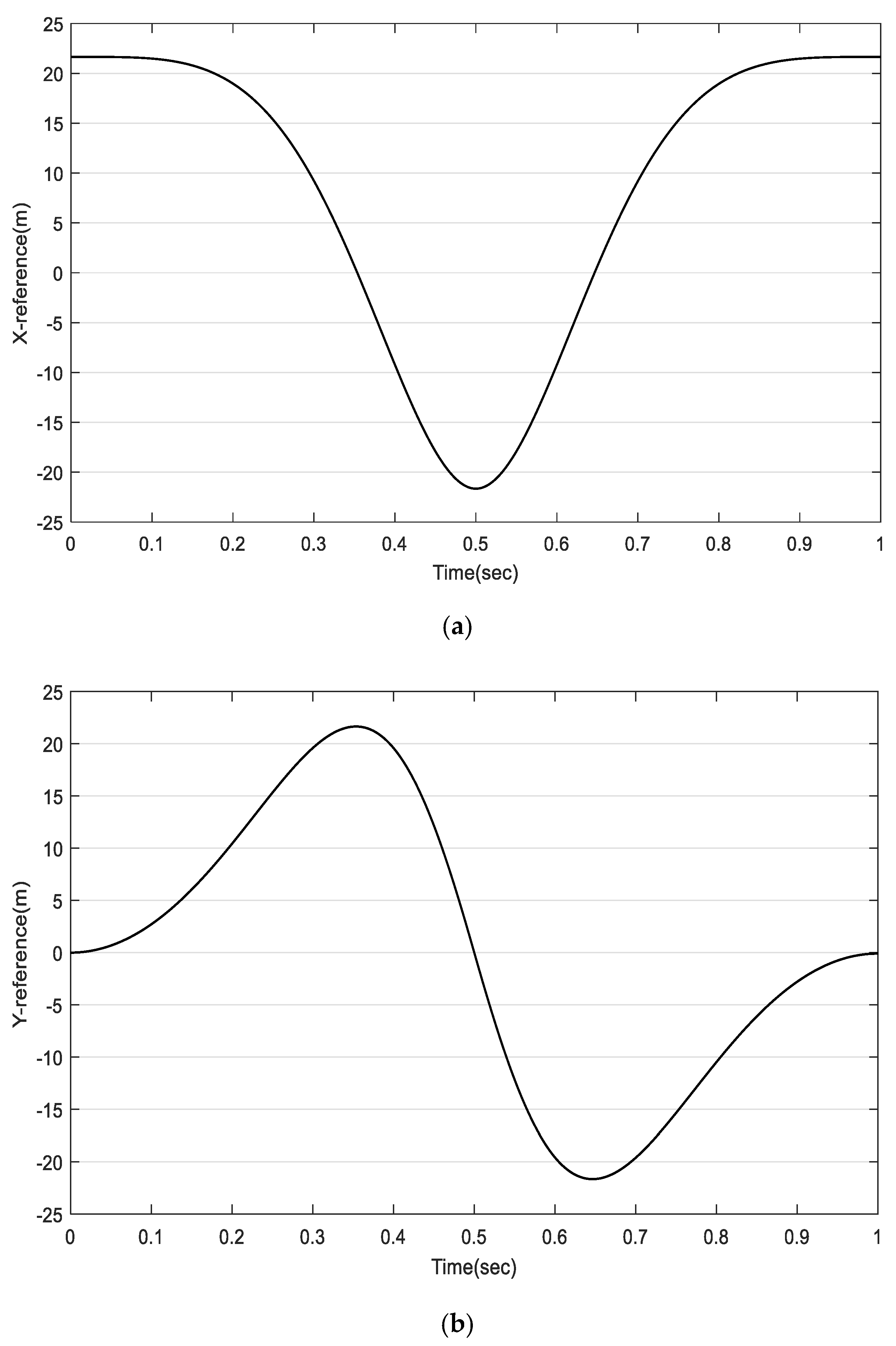
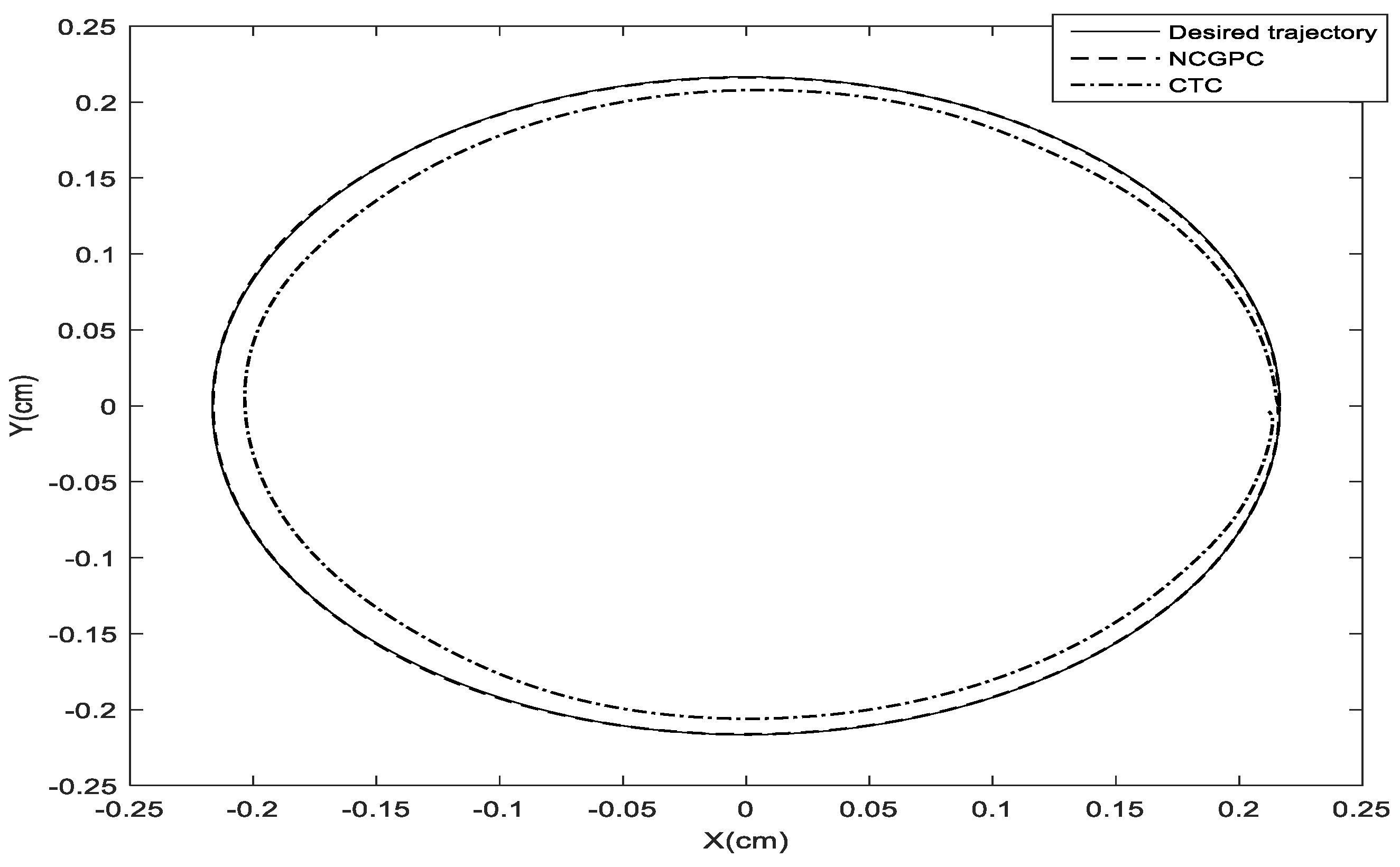
S ( X ) is the pseudo-inverse of   S ( X ) . The reference trajectory is chosen as a circular path given by
{ x m r e f = 0.2165 s i n ( α ( t ) ) y m r e f = 0.2165 c o s ( α ( t ) )
where α ¨ ( t ) = 8 π ,   α ( 0 ) = α ˙ ( 0 ) = 0 .
Referring to Table 1, the parameters for the dynamic Equation (34) for both the 4-cable CDDRs are assumed as mass m = 0.01 kg and rotational shaft/pulley inertias Ji (i = 1, …, 4) = 0.0008 kg m2. Shaft rotational viscous damping coefficients Ci (i = 1, …, 4) = 0.01 Nm s and ri = r = 1 cm (for all i = 1, …, 4), and the base square side is Lb = 0.658 m, as also summarized in Table 3. We defined the reference frame of our CDPR system in the center of the workspace with coordinates (0,0).
Figure 4 shows the plots of the reference trajectory for X- and Y-coordinates. The proposed simulation study was carried out with three phases:
  • Phase 1: Influence of the prediction horizon on NCGPC tracking performances.
  • Phase 2: Comparison between NCGPC and CTC based on tracking errors.
  • Phase 3: Robustness test of payload and parameter uncertainties for both NCGPC and CTC.

5.1. Influence of the Prediction Horizon on NCGPC Tracking Performances

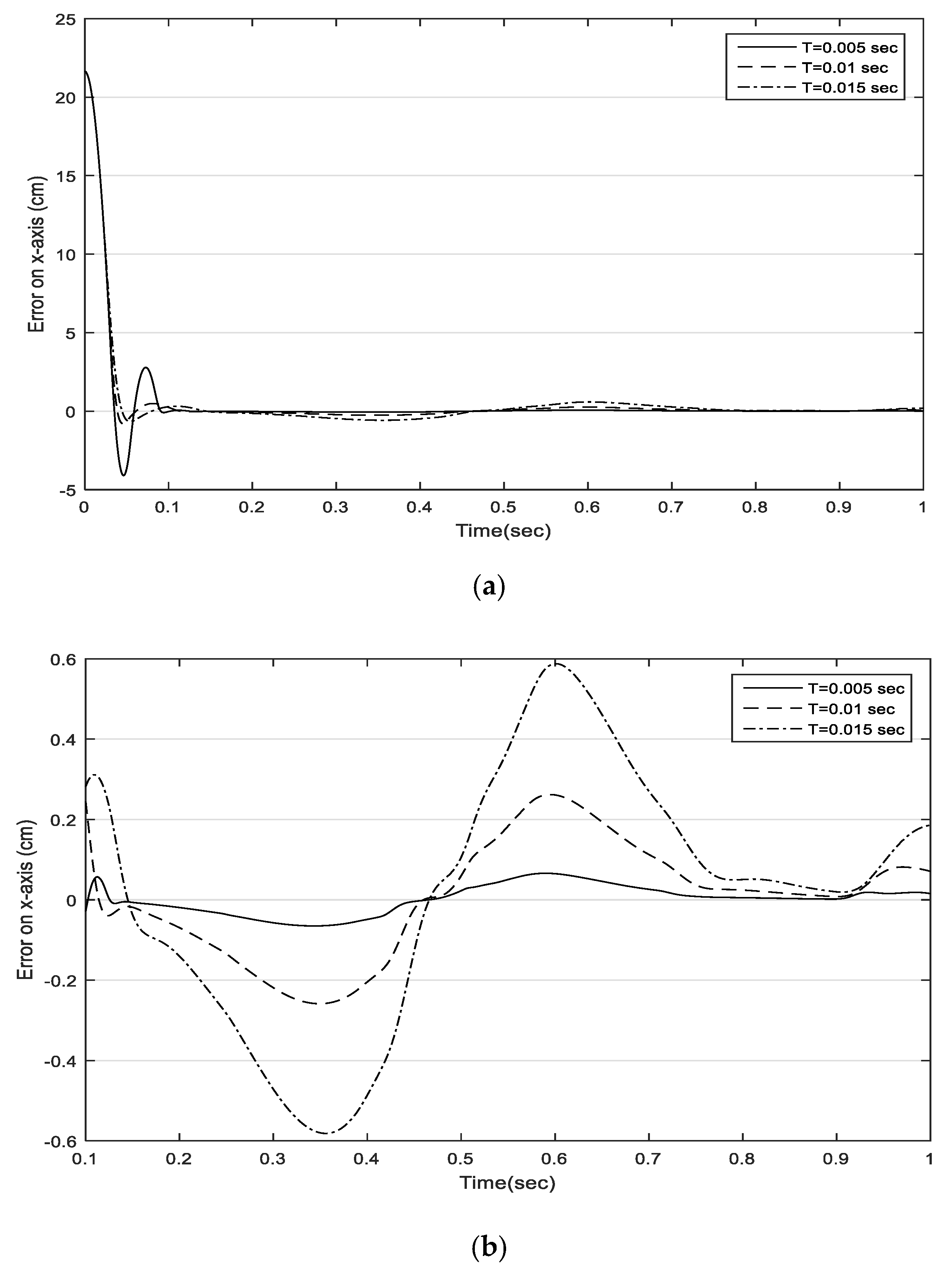
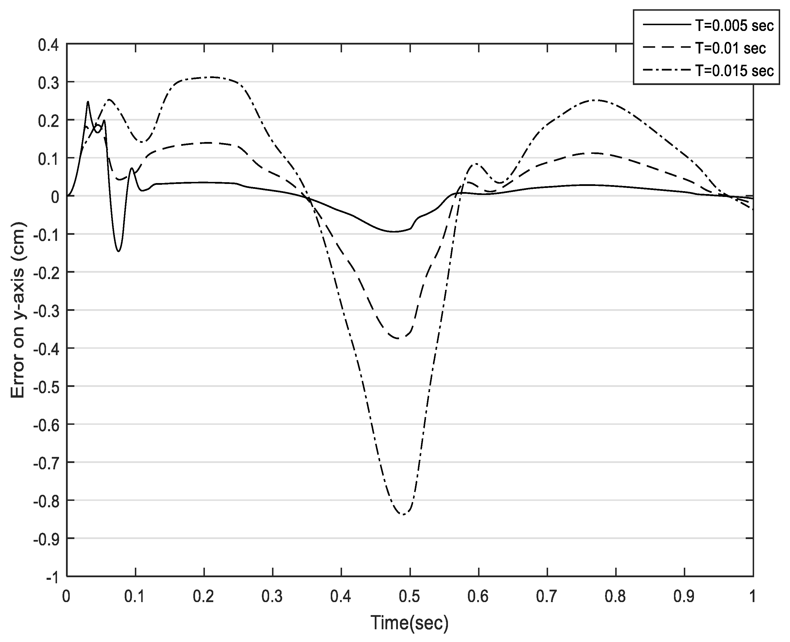
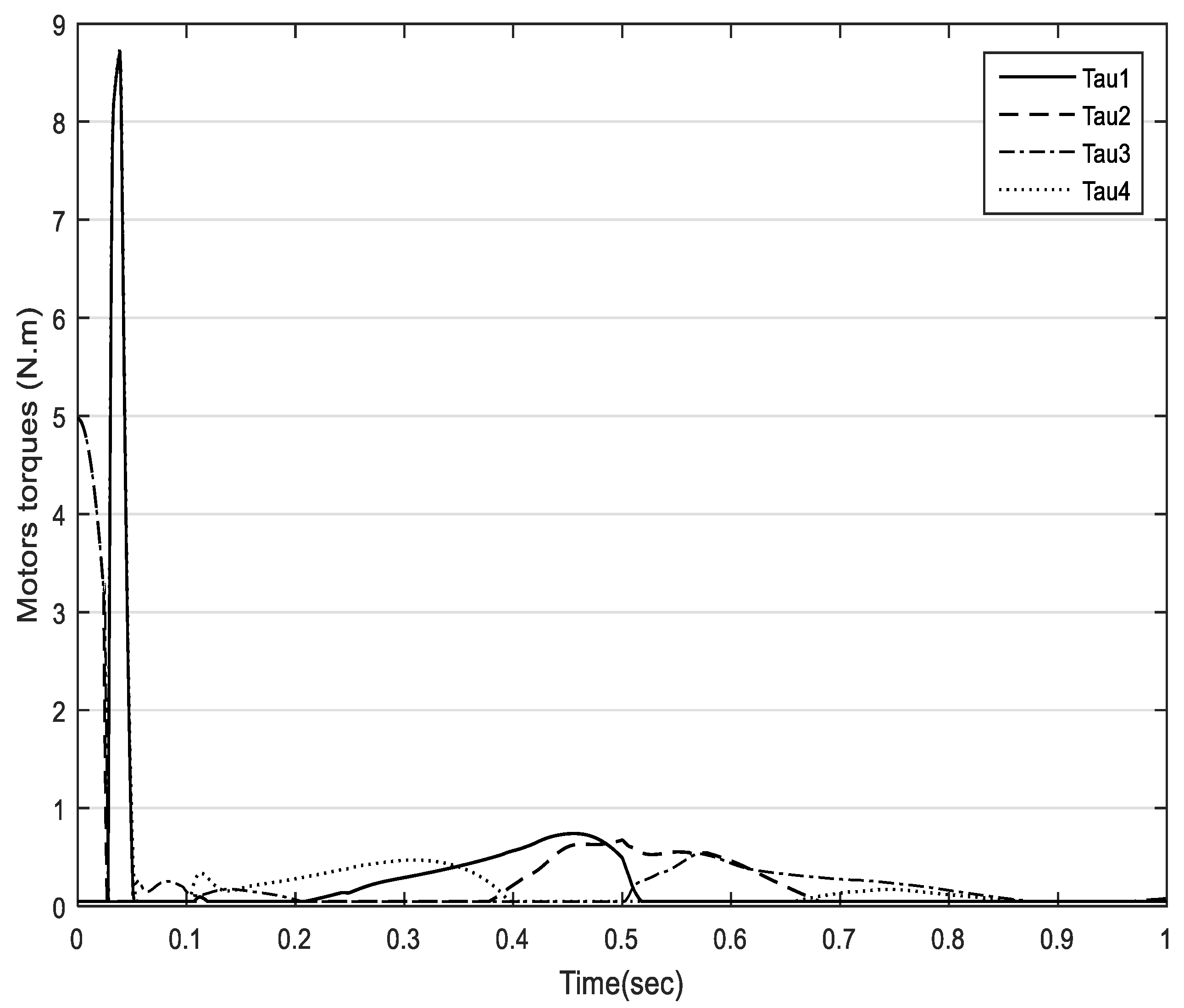
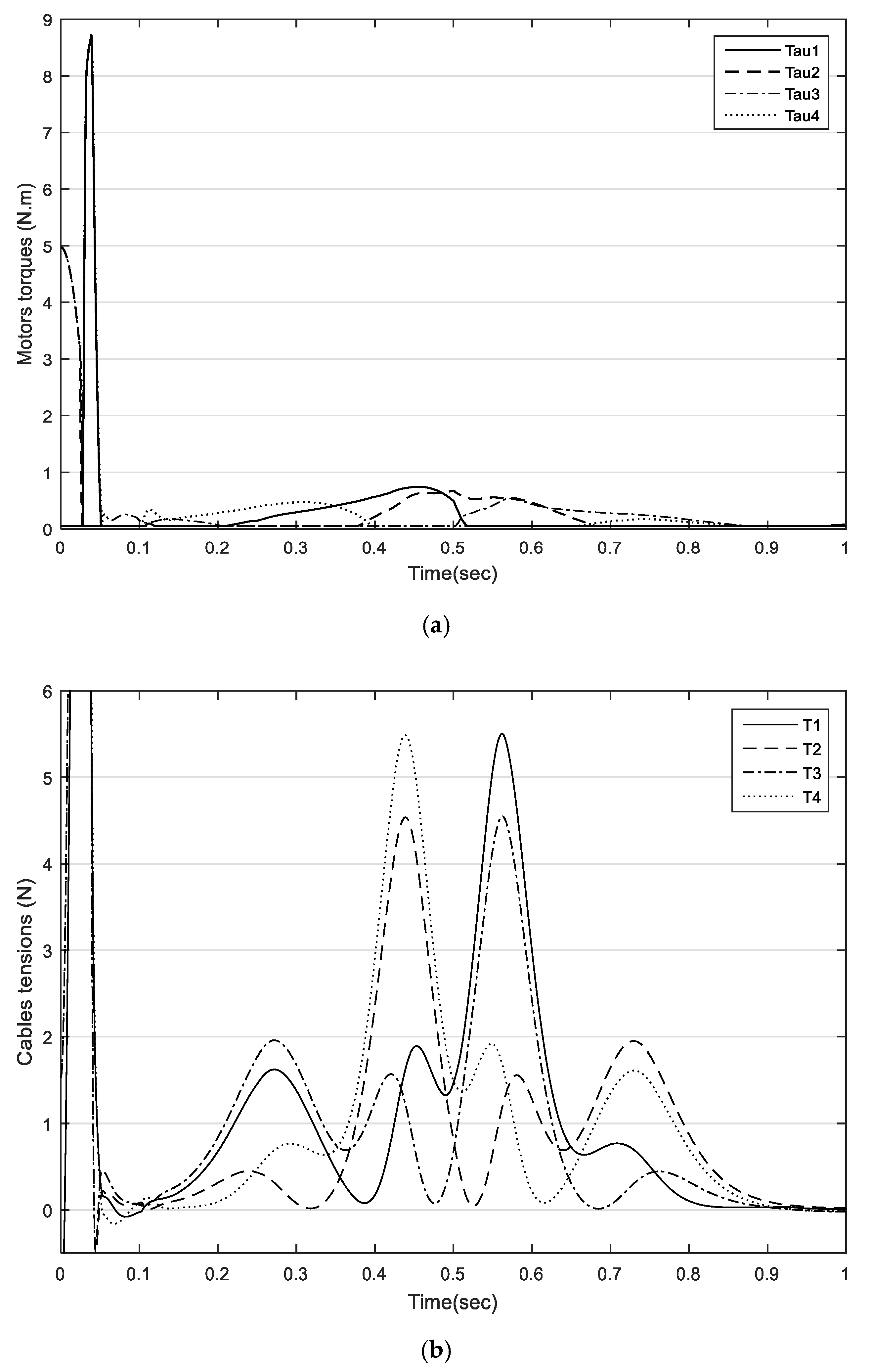
Figure 5 shows tracking errors on the X-axis for different prediction horizons and a zoom on X-axis tracking errors (b). Figure 5 and Figure 6 show the tracking performances that can be achieved by the proposed NCGPC control with a maximum error lower than 0.6 cm on the X-axis and 0.9 cm on the Y-axis in the worst case at t = 0.015 s. The prediction horizon exerts a direct influence on the transient response because it acts directly on the pole placement of the closed loop. In addition, the steady state error is affected by the prediction horizon, which is due to the precision decrease in the prediction model when the prediction horizon becomes longer. In Figure 7, motor torques are shown. The lower and upper bounds are limited (between 0.01–10 Nm) to avoid negative and high tensions, which can lead to a cable loosening or tearing. Figure 8 shows resulting tensions in robot cables. Cable tensions are positive, except in the transient response, where they are slightly negative.

5.2. Comparison between NCGPC and CTC Based on Tracking Errors

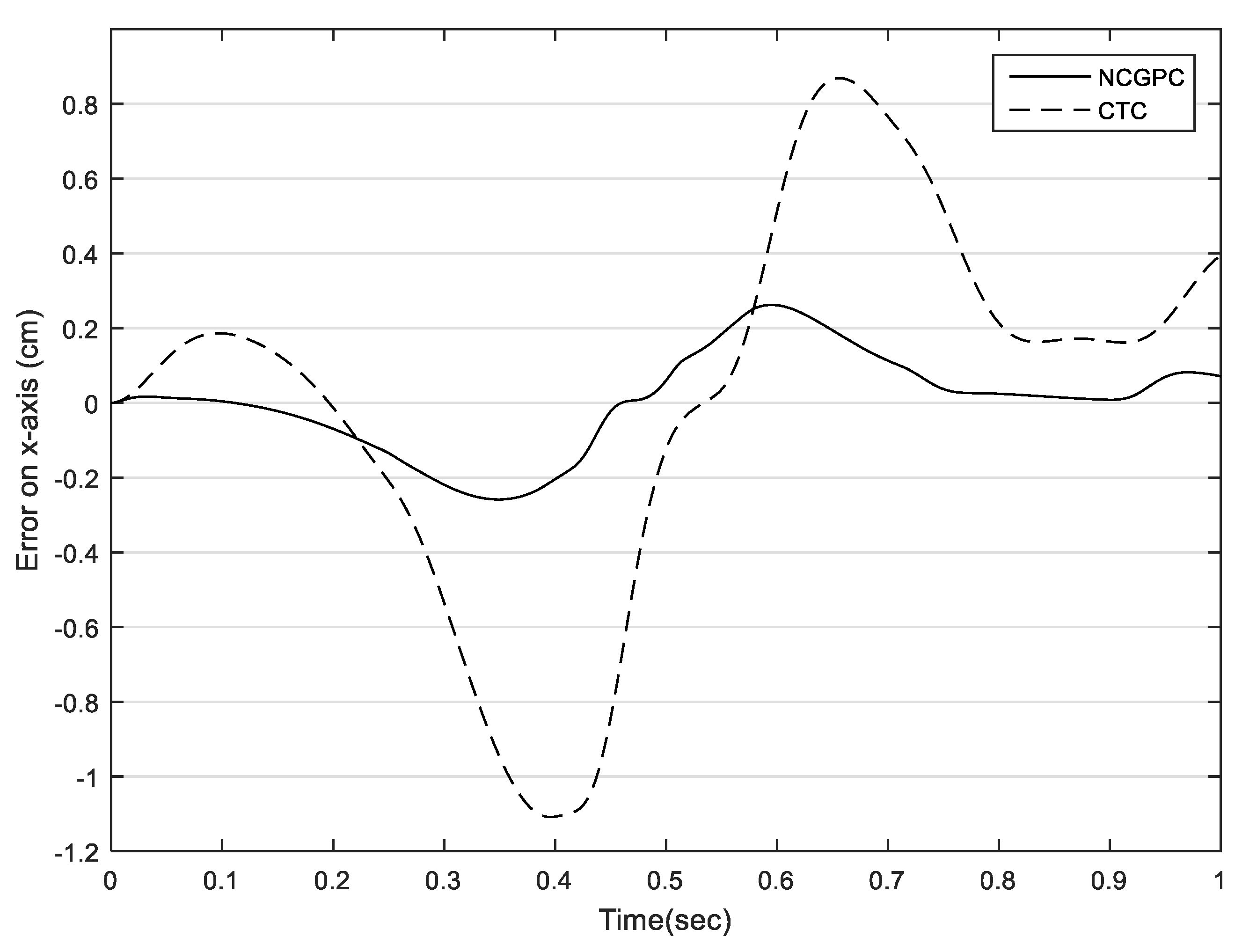
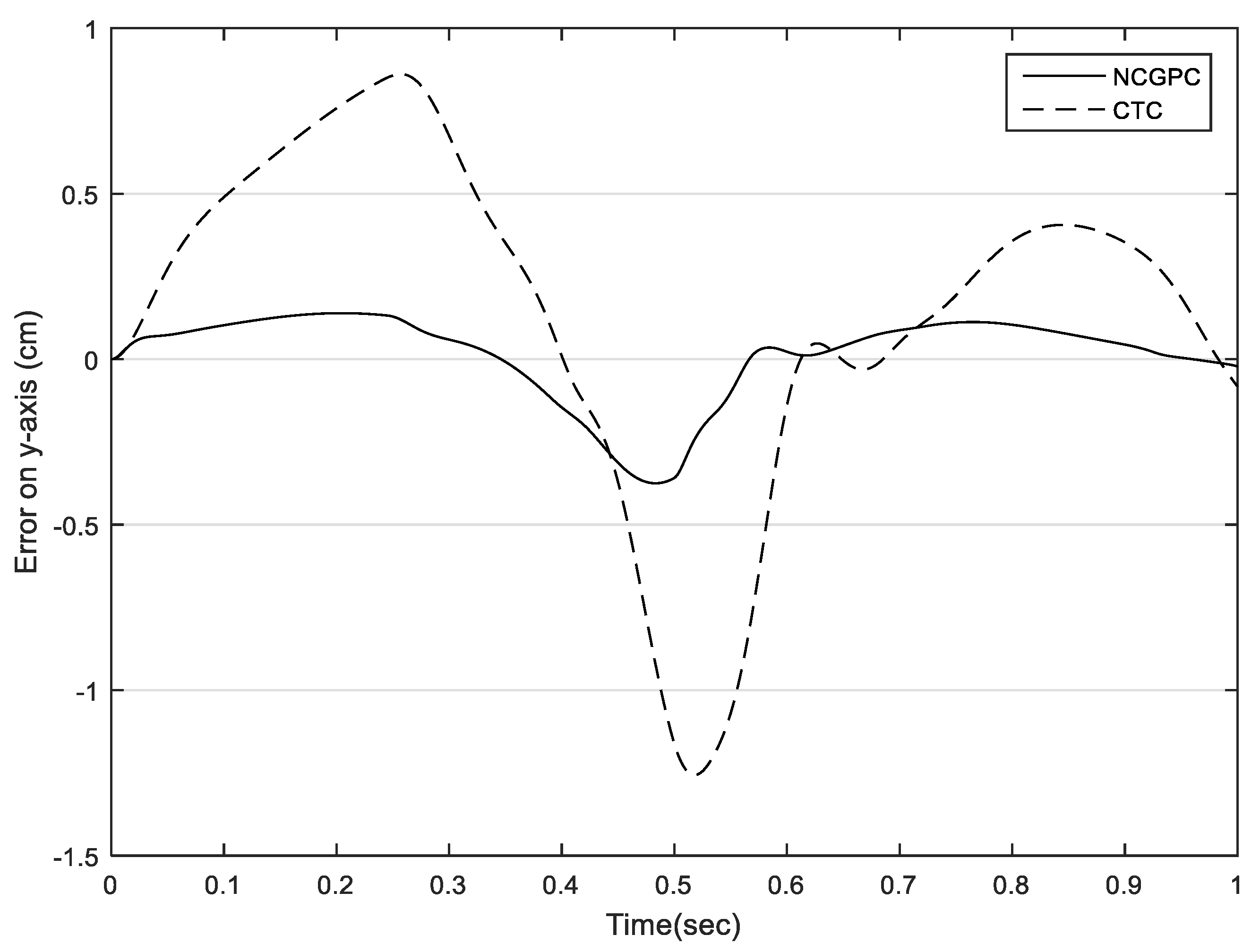
Figure 9 and Figure 10 show the tracking errors along X- and Y-directions of the end-effector under different control strategies. In order to illustrate the superiority of the NCGPC scheme, we compared it with CTC. In particular, one can identify a positioning error ranging from +0.2 to +0.4 cm for the NCGPC control method, while one can identify a positioning error ranging from −1.3 to +0.8 cm for the CTC control. One can also compute the least square average positioning error along the X-axis as 0.04 cm with NCGPC and 0.2 cm with CTC when referring to the interval from 0.0 to 0.3 s. The least square average positioning error along the X-axis is 0.2 cm with NCGPC and 0.8 cm with CTC when referring to the interval from 0.5 to 0.8 s. Similarly, the least square average positioning error along the X-axis is 0.2 cm with NCGPC and 0.8 cm with CTC when referring to the interval from 0.0 to 0.3 s. The least square average positioning error along the X-axis is 0.1 cm with NCGPC and 0.4 cm with CTC when referring to the interval from 0.5 to 0.8 s.
As seen for these values, we can conclude that the NCGPC has a higher position tracking accuracy compared with other control methods with different prediction horizons. One should note that NCGPCs are extended from affine nonlinear systems to general nonlinear systems and strategies applied to a permanent magnet motor for speed trajectory tracking and disturbance rejection. Furthermore, they are revised in order to enhance the robustness of the closed-loop system. Computed torque control (CTC) is instead an effective and high-performance motion control strategy for a robotic system. Based on the simulation error results, we can conclude that the proposed control method is effective and robust and can outperform CTC.

5.3. Robustness Test of Payload and Parameter Uncertainties

Measurement uncertainty is a nonnegative parameter characterizing the dispersion of the quantity values attributed to a measure and based on the information used. The guide to the expression of uncertainty in measurement (GUM) is the internationally accepted reference for evaluating uncertainty, and it requires the use of a first-order Taylor series expansion for propagating uncertainties. The specific assumed uncertainty values are reported in Table 4.
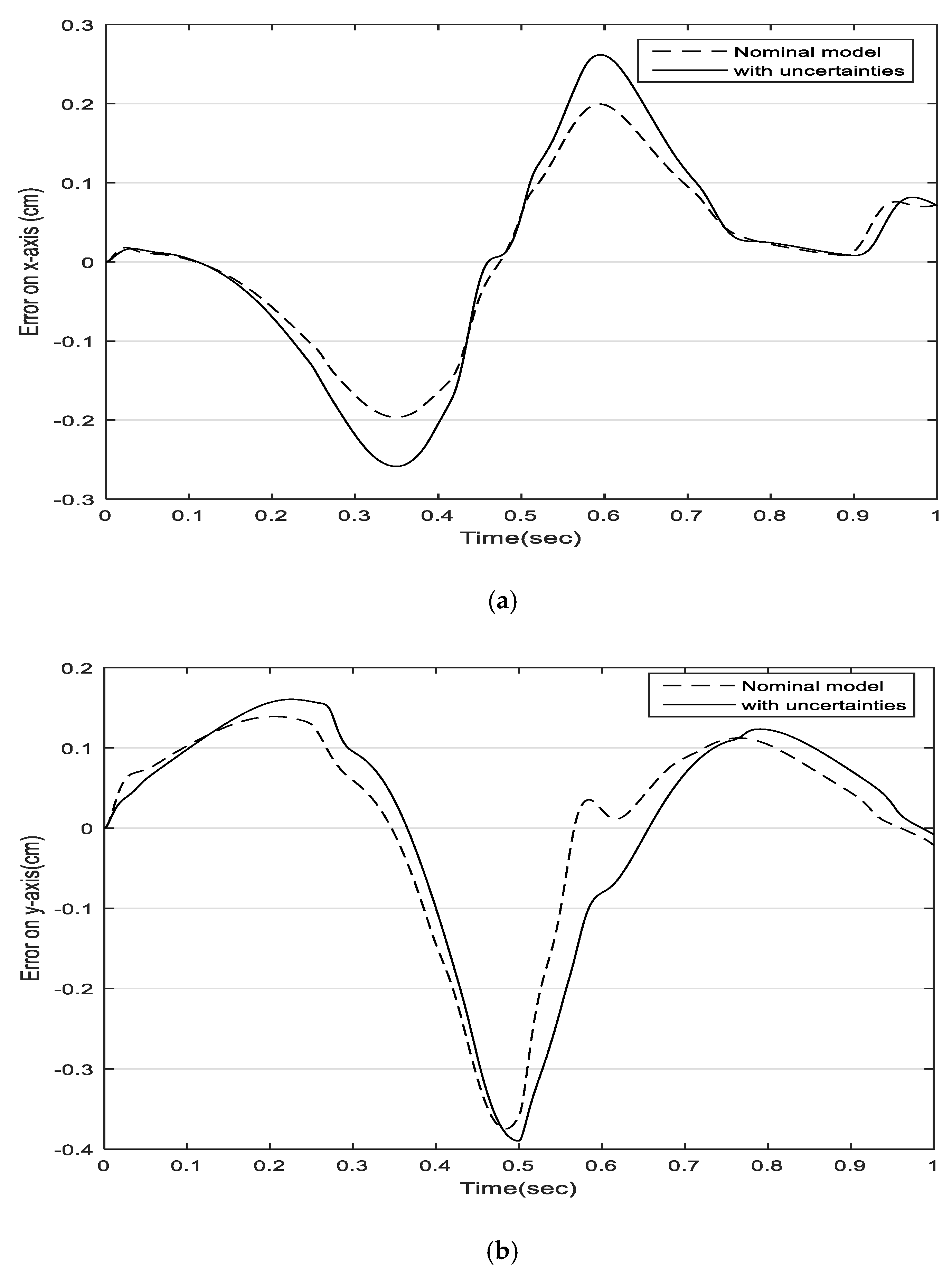
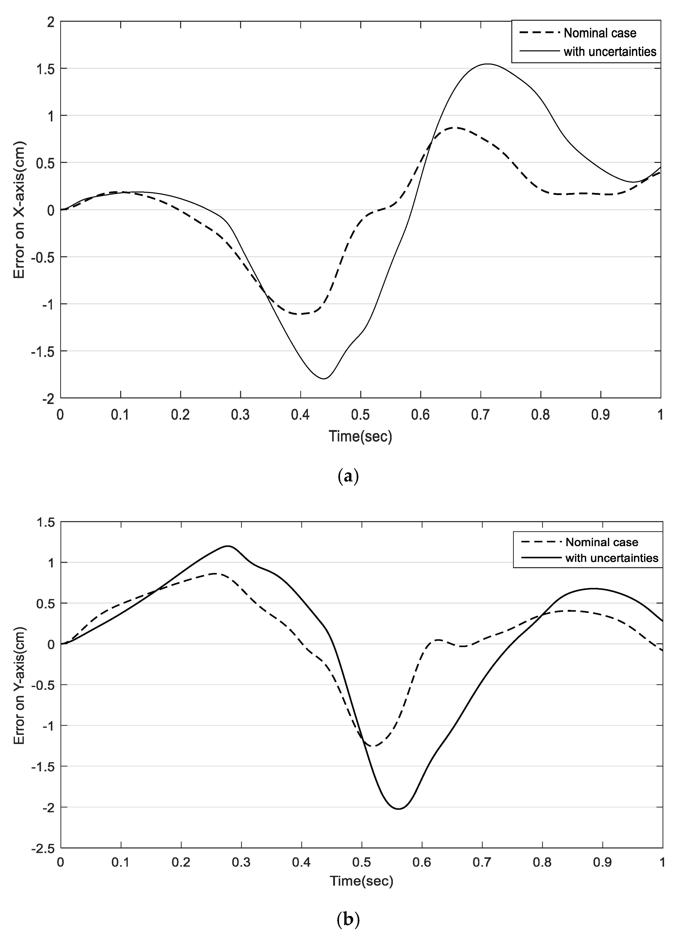
The introduced uncertainties, which were implemented in numerical modeling with Matlab Simulink software, are given in Table 4. Using the proposed robust control toolbox, one can analyze the effect of model uncertainty on the closed-loop stability and performance of the control system. In particular, one can determine whether our controller will perform adequately over the entire considered operating range, and which source of uncertainty is most likely to jeopardize the performance. The considered uncertainties are mostly related to the cable lengths. Cables can only pull, so there are only feasible positive cable tensions. The elasticity of cables makes them elongate proportionally to cable tensions. Accordingly, only positive increases in the cable lengths can be feasible under positive cable tensions as compared with nominal values. Although a sensitivity analysis is out of the scope of this work, the proposed formulation allows for tolerances in the setup parameters commonly above 1% of full scale, as reported in the plots in Figure 11, Figure 12, Figure 13 and Figure 14.
We noticed that the position versus time curves obtained with the NCGPC method with the uncertainties follow (superpose to) the curve of the nominal model in the interval from 0.0 to 0.2 s very well. Similarly, in the interval from 0.22 to 0.4 s, we observe that the model with uncertainties follows the curve of the nominal NCGPC control model very well, with a similar tracking error ranging between 0.03 to 0.05 cm. In the interval from 0.5 to 1 s, the curve of NCGPC with uncertainties follows the curve of the nominal model with a maximum tracking error of 0.04 cm along both the X- and Y- directions. On the other hand, the position versus time curves obtained with the CTC method when considering the same uncertainties demonstrate a significantly different behavior; that is, the interval from 0.0 to 2.0 s shows a similar tracking performance but starting from the interval from 0.02 to 0.1, the curve with uncertainties demonstrates a significantly worst tracking error performance with a large tracking error between 0.03 and 1 cm along both the X- and Y-directions. When compared to Figure 9 and Figure 10, the position tracking errors along the X-direction with the NCGPC method show a tracking error performance that is 98% better than the CTC in the interval from 0 to 2 s, where the tracking error results are negligible for NCGPC, while it is 0.2 cm with the CTC method. Similarly, the NCGPC control method shows a performance improvement as compared with the CTC method of about 90% in several specific time intervals. Considering absolute values, for example, NCGPC shows a tracking error of −0.23 cm, while CTC shows a tracking error of 1.16 cm at the time 4 s. Similarly, along the Y-direction at time 0.25 s, NCGPC shows a tracking error of 0.13 cm, while CTC shows a tracking error of 0.94 cm, again with NCGPC outperforming CTC by about 90%. Accordingly, one can outline that, when introducing model uncertainties and payload mass, NCGPC demonstrates a significant improvement in tracking error performance as compared with a standard CTC, also in the presence of significant amounts of uncertainties.
In this paper, the existing results for the analytic NCGPC are extended from affine nonlinear systems to general nonlinear systems (the proposed CDPR robot). This controller overcomes the difficulties imposed by the on-line nonlinear optimization involved in NNCGPC, such as attaining local-minimum and long-sampling-time requirements. The NCGPC developed in this paper is suboptimal for the original NCGPC problem. Since there is no restriction on the order for Taylor-series expansion, theoretically, the analytic solution developed by approximation can approach the solution of the original NCGPC at any specified accuracy.
This study is mostly focused on a specific planar CDPR. In future work, we plan to extend this formulation to a 3D CDPR, such as LAWEX and CUBE, with 3 to 6 active degrees of freedom; to reconfigurable cable-driven devices; and/or to devices with new application tasks, such as those reported in [36,37,38,39,40,41]. Additionally, multiobjective optimization strategies could be implemented at design and control stages, as proposed, for example, in [42,43].

6. Conclusions

This paper describes a novel continuous time predictive controller design method for a planar cable-driven parallel robot. The proposed method is based on the minimization of a quadratic cost function of the predicted tracking error as calculated using Taylor expansion. The main advantages of this proposed control scheme consist of avoiding on-line optimizations and the capability to deal with fast dynamics on nonlinear systems. Simulation results showed that the proposed NCGPC technique has a significantly improved tracking performance with respect to a standard computed torque control (CTC). Furthermore, the proposed control method demonstrates a suitable robustness in terms of the rejection of model uncertainties and payload variations, as also demonstrated in comparison with a CTC controller.

Author Contributions

Conceptualization, F.I. and G.C.; software, F.I. and A.M.; writing—original draft preparation, F.I. and A.M.; writing—review and editing, G.C., supervision, G.C.; All authors have read and agreed to the published version of the manuscript.

Funding

This research received no external funding

Institutional Review Board Statement

Not applicable.

Informed Consent Statement

Not applicable.

Data Availability Statement

Not applicable.

Conflicts of Interest

The authors declare no conflict of interest.

References

  1. Albus, J.; Bostelman, R.; Dagalakis, N. The NIST RoBoCrane. J. Res. Natl. Inst. Stand. Technol. 1992, 94, 373–384. [Google Scholar] [CrossRef] [PubMed]
  2. Tang, X. An Overview of the Development for Cable-Driven Parallel Manipulator. Adv. Mech. Eng. 2014, 6, 823028. [Google Scholar]
  3. Pinto, A.M.; Moreira, E.; Lima, J.; Sousa, J.P.; Costa, P. A cable-driven robot for architectural constructions: A visual-guided approach for motion control and path-planning. Auton. Robots 2017, 41, 1487–1499. [Google Scholar] [CrossRef]
  4. Morizono, T.; Kurahashi, K.; Kawamura, S. Realization of a Virtual Sports Training System with Parallel Wire Mechanism. In Proceedings of the International Conference on Robotics and Automation, Albuquerque, NM, USA, 21–27 April 1997; Volume 4, pp. 3025–3030. [Google Scholar]
  5. Reddy, M.V.; Praneet, N.C.; Ananthasuresh, G.K. Planar Cable-Driven Robots with Enhanced Orientability. In Cable-Driven Parallel Robots Mechanisms and Machine Science 74; Springer Nature: Cham, Switzerland, 2019; pp. 3–12. [Google Scholar]
  6. Korayem, M.; Yousefzadeh, M.; Tourajizadeh, H. Optimal Control of a Wheeled Mobile Cable-Driven Parallel Robot ICaSbot with Viscoelastic Cables. Robotica 2020, 38, 1513–1537. [Google Scholar] [CrossRef]
  7. Wei, H.; Qiu, Y.; Sheng, Y. On the Cable Pseudo-Drag Problem of Cable-Driven Parallel Camera Robots at High Speeds. Robotica 2019, 37, 1695–1709. [Google Scholar]
  8. Hwang, S.; Bak, J.; Yoon, J.; Park, J. Oscillation Reduction and Frequency Analysis of Under-Constrained Cable-Driven Parallel Robot with Three Cables. Robotica 2020, 38, 375–395. [Google Scholar] [CrossRef]
  9. Laroche, E.; Chellal, R.; Cuvillon, L.; Gangloff, J. A preliminary study for H∞ control of parallel cable-driven manipulators. Cable Driven Parallel Robot. Mech. Mach. Sci. 2013, 12, 353–369. [Google Scholar]
  10. Khosravi, M.A.; Taghirad, H.D. Dynamic analysis and control of cable driven robots with elastic cables. Trans. Can. Soc. Mech. Eng. 2011, 35, 543–558. [Google Scholar] [CrossRef] [Green Version]
  11. Korayem, M.H.; Tourajizadeh, H.; Taherifar, M.; Korayem, A.H. Optimal feedback linearization control of a flexible cable robot. Lat. Am. Appl. Res. 2014, 44, 259–265. [Google Scholar]
  12. Li, B.; Yan, L.; Gerada, C. The Novel Singular-Perturbation-Based Adaptive Control with σ-Modification for Cable Driven System. Actuators 2021, 10, 45. [Google Scholar] [CrossRef]
  13. Fernández, J.D.; Yu, B.; Bargsten, V.; Zipper, M.; Sprengel, H. Design, Modelling and Control of Novel Series-Elastic Actuators for Industrial Robots. Actuators 2020, 9, 6. [Google Scholar]
  14. Deng, E.; Tadesse, Y. A Soft 3D-Printed Robotic Hand Actuated by Coiled SMA. Actuators 2021, 10, 6. [Google Scholar] [CrossRef]
  15. Laribi, A.; Carbone, G.; Zeghloul, S. On the Optimal Design of Cable Driven Parallel Robot with a Prescribed Workspace for Upper Limb Rehabilitation Tasks. J. Bionic Eng. 2019, 16, 503–513. [Google Scholar] [CrossRef]
  16. Inel, F.; Menssouri, Z.; Carbone, G.; Ceccarelli, M. Dynamic Modeling and Simulation of Sliding Mode Control for a Cable Driven Parallel Robot. In New Advances in Mechanism and Machine Science; Springer: Cham, Switzerland, 2018; Volume 57, pp. 413–426. [Google Scholar]
  17. Carbone, G.; Gherman, B.; Ulinici, I.; Vaida, C.; Pisla, D. Design issues for an inherently safe robotic rehabilitation device. In New Advances in Mechanism and Machine Science; Springer: Cham, Switzerland, 2018; Volume 49, pp. 1025–1032. [Google Scholar]
  18. Tang, X.Q.; Shao, Z.F. Trajectory generation and tracking control of a multi-level hybrid support manipulator in FAST. Mechatronics 2013, 23, 1113–1122. [Google Scholar] [CrossRef]
  19. Li, M.; Wu, H.; Wang, Y.; Handroos, H.; Carbone, G. Modified Levenberg-Marquardt algorithm for backpropagation neural network training in dynamic model identification of mechanical systems. J. Dyn. Syst. Meas. Control Trans. ASME 2017, 139. [Google Scholar] [CrossRef]
  20. Poignet, P.; Gautier, M. Nonlinear model predictive control of a robot manipulator. In Proceedings of the 6th International Workshop on Advanced Motion Control. Proceedings (Cat. No.00TH8494), Nagoya, Japan, 30 March–1 April 2000; pp. 401–406. [Google Scholar] [CrossRef]
  21. Chen, W.H. Predictive Control of General Non-linear Systems Using Approximation. IEEE Proc. Control Theory Appl. 2004, 151, 137–144. [Google Scholar] [CrossRef] [Green Version]
  22. Hedjar, R.; Toumi, R.; Boucher, P.; Dumur, D. Finite Horizon Non-linear Predictive Control by the Taylor Approximation Application to Robot Tracking Trajectory. Int. J. Appl. Math. Comput. Sci. 2005, 15, 527–540. [Google Scholar]
  23. Zhao, L.; Li, Q.; Liu, B.; Cheng, H. Trajectory tracking control of a one degree of freedom manipulator based on a switched sliding mode controller with a novel extended state observer framework. IEEE Trans. Syst. Man Cybernet. Syst. 2019, 49, 1110–1118. [Google Scholar] [CrossRef]
  24. Dabo, M.; Chafouk, H.; Langlois, N. Unconstrained NCGPC with a Guaranteed Closed-Loop Stability: Case of Non-linear SISO Systems with the Relative Degree Greater than Four. In Proceedings of the 48th IEEE Conference on Decision and Control, Shanghai, China, 15–18 December 2009; pp. 1980–1985. [Google Scholar]
  25. Siller-Alcalá, I.I.; Liceaga-Castro, J.U. Continuous Time Generalized Predictive Control from a Classical Control Perspective. WSEAS Trans. Syst. Control 2018, 13, 447–452. [Google Scholar]
  26. Carbone, G.; Aróstegui Cavero, C.; Ceccarelli, M.; Altuzarra, O. A study of feasibility for a limb exercising device. In New Advances in Mechanism and Machine Science; Springer: Cham, Switzerland, 2018; Volume 47, pp. 11–21. [Google Scholar]
  27. Errouissi, R.; Ouhrouche, M.; Chen, W.-H. Robust Non-linear Generalized Predictive Control of a Permanent Magnet Synchronous Motor with an Anti-Windup Compensator. In Proceedings of the IEEE International Symposium on Industrial Electronics (ISIE), Bari, Italy, 4–7 July 2010; pp. 3184–3189. [Google Scholar]
  28. Krid, M.; Benamar, F.; Lenain, R. A New Explicit Dynamic Path Tracking Controller Using Generalized Predictive Control. Int. J. Control Automat. Syst. 2017, 15, 303–314. [Google Scholar]
  29. Siller-Alcalá, I.I.; Liceaga-Castro, J.U.; Alcántara-Ramírez, R.; Jaimes-Ponce, J. Non-linear Control of a Single-Link Flexible Joint Manipulator via Predictive Control. WSEAS Trans. Syst. Control 2016, 11, 371–375. [Google Scholar]
  30. Wang, H.; Li, S.; Lan, Q.; Zhao, Z.; Zhou, X. Continuous terminal sliding mode control with extended state observer for PMSM speed regulation system. Trans. Inst. Meas. Control 2017, 39, 1195–1204. [Google Scholar] [CrossRef]
  31. Piao, J.; Kim, E.; Choi, H.; Moon, C.; Choi, E.; Park, J.; Kim, C.-S. Indirect Force Control of a Cable-Driven Parallel Robot Tension Estimation using Artificial Neural Network trained by Force Sensor Measurements. Sensors 2019, 19, 2520. [Google Scholar] [CrossRef] [Green Version]
  32. Jin, X.; Jung, J.; Ko, S.Y.; Choi, E.; Park, J.-O.; Kim, C.-S. Geometric Parameter Calibration for a Cable-Driven Parallel Robot Based on a Single One-Dimensional Laser Distance Sensor Measurement and Experimental Modeling. Sensors 2018, 18, 2392. [Google Scholar]
  33. Piao, J.; Jin, X.; Jung, J.; Choi, E.; Park, J.-O.; Kim, C.-S. Open-loop position control of a polymer cable–driven parallel robot via a viscoelastic cable model for high payload workspaces. Adv. Mech. Eng. 2017, 9, 1–12. [Google Scholar] [CrossRef] [Green Version]
  34. Cafolla, D.; Russo, M.; Carbone, G. CUBE, a Cable-driven Device for Limb Rehabilitation. J. Bionic Eng. 2019, 16, 493–494. [Google Scholar] [CrossRef]
  35. Kumar, R.; Mukherjee, S. Enhanced Dynamic Capability of Cable-Driven Parallel Manipulators by Reconfiguration. Robotica 2021, 1–9. [Google Scholar] [CrossRef]
  36. Mu, Z.; Liu, T.; Xu, W.; Lou, Y.; Liang, B. Dynamic feedforward control of spatial cable-driven hyper-redundant manipulators for on-orbit servicing. Robotica 2019, 37, 18–38. [Google Scholar] [CrossRef]
  37. Yao, S.; Ceccarelli, M.; Carbone, G.; Dong, Z. Grasp configuration planning for a low-cost and easy-operation under actuated three-fingered robot hand. Mech. Mach. Theory 2018, 129, 51–69. [Google Scholar] [CrossRef]
  38. Gherman, B.; Birlescu, I.; Plitea, N.; Carbone, G.; Tarnita, D.; Pisla, D. On the singularity-free workspace of a parallel robot for lower-limb rehabilitation. Proc. Roman. Acad. Series A Math. Phys. Techn. Sci. Inform. Sci. 2019, 20, 383–391. [Google Scholar]
  39. Boschetti, G.; Carbone, G.; Passarini, C. Cable failure operation strategy for a rehabilitation cable-driven robot. Robotics 2019, 8, 17. [Google Scholar] [CrossRef] [Green Version]
  40. Hernández-Martínez, E.E.; Ceccarelli, M.; Carbone, G.; López-Cajún, C.S.; Jáuregui-Correa, J.C. Characterization of a cable-based parallel mechanism for measurement purposes. Mech. Based Design Struct. Mach. 2010, 38, 25–49. [Google Scholar] [CrossRef]
  41. Tucan, P.; Vaida, C.; Ulinici, I.; Banica, A.; Burz, A.; Pop, N.; Birlescu, I.; Gherman, B.; Plitea, N.; Antal, T.; et al. Optimization of the ASPIRE Spherical Parallel Rehabilitation Robot Based on Its Clinical Evaluation. Int. J. Environ. Res. Public Health 2021, 18, 3281. [Google Scholar] [CrossRef]
  42. Vaida, C.; Birlescu, I.; Pisla, A.; Ulinici, I.; Tarnita, D.; Carbone, G.; Pisla, D. Systematic design of a parallel robotic system for lower limb rehabilitation. IEEE Access 2020, 8, 34522–34537. [Google Scholar] [CrossRef]
  43. Ceccarelli, M.; Carbone, G.; Ottaviano, E. Multi criteria optimum design of manipulators. Bull. Polish Acad. Sci. Techn. Sci. 2019, 53, 9–18. [Google Scholar]
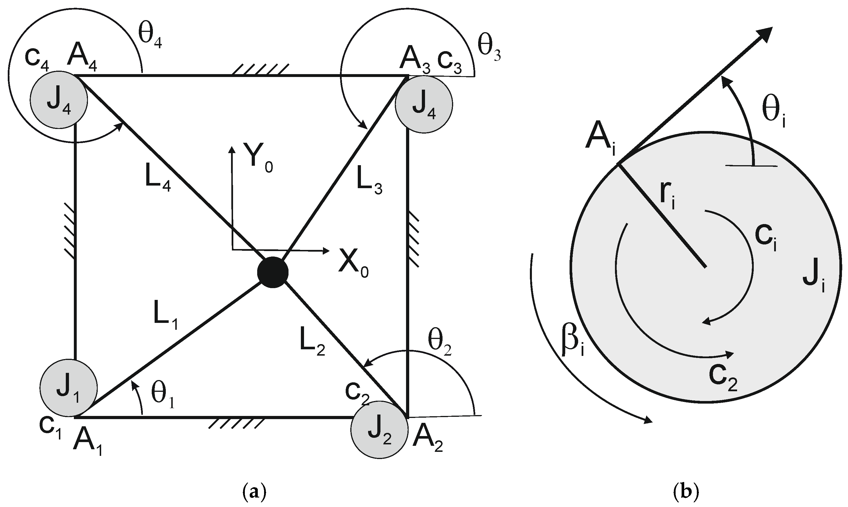
Figure 1. (a) Planar four-cable-driven parallel robot structure. (b) The structure diagram of the pulley/shaft system.
Actuators 10 00097 g001
Figure 2. A flow-chart of tension control (NCGPC: nonlinear continuous time generalized predictive control; PDP robots: planar-driven parallel robots).
Actuators 10 00097 g002
Figure 3. Proposed control schemes for the proposed planar 4-cable CDPR.
Actuators 10 00097 g003
Figure 4. A plot of the reference trajectory: (a) X-coordinate; (b) Y-coordinate.
Actuators 10 00097 g004
Figure 5. (a) NGPC tracking errors on X-axis for different prediction horizons. (b) Zoom on X-axis tracking errors.
Actuators 10 00097 g005
Figure 6. NGPC tracking errors on Y-axis for different prediction horizons.
Actuators 10 00097 g006
Figure 7. Motors torques produced by NGPC for T = 0.01 s.
Actuators 10 00097 g007
Figure 8. (a) Cables tensions. (b) Zoom on cable tensions.
Actuators 10 00097 g008
Figure 9. Position tracking errors along X-direction.
Actuators 10 00097 g009
Figure 10. Position tracking errors along Y-direction.
Actuators 10 00097 g010
Figure 11. Effect of model uncertainties on NCGPC tracking errors: (a) X-axis; (b) Y-axis.
Actuators 10 00097 g011
Figure 12. Desired and actual trajectories in task space.
Actuators 10 00097 g012
Figure 13. Effect of model uncertainties on CTC tracking errors: (a) X-axis; (b) Y-axis.
Actuators 10 00097 g013
Figure 14. Effect of model uncertainties on both CTC and NCGPC tracking performance.
Actuators 10 00097 g014
Table 1. Nomenclature of the robot geometric parameters.
ParametersNomenclature
A i = ( A ix , A iy ) Attachment points of the driving cables to the motorized pulleys.
L i Driven   cables   lengths
θ i Cables angles with respect to the x-axis.
L B The lengths of the workspace side.
X m End-effector’s x-coordinate.
Y m End-effector’s y-coordinate.
M End-effector’s mass.
Τ i Motors torques.
J i Rotational inertia of shaft-pulley system.
C i Motors shafts viscous damping coefficients.
β i Pulleys’ rotation angles.
r i Pulleys radius.
Table 2. Nomenclature of the multiple input–multiple output (MIMO) system parameters variables.
ParametersNomenclature
xthe states vector
Ucontrol vector
youtput vector
F(x) and h(x)smooth vector fields
y (t + T)future reference
e (t + T)future tracking error vector
yr (t + T)quadratic performance
i s the last row of the matrix
i ss is the last element of i s
K i is the ( ρ i × 1 ) gain vector
ρirelative degree
Table 3. Main values of parameters for the proposed case study.
ParametersValueParametersValue
( A 1 x , A 1 y ) (−32.5;0) cm L B 65 cm
( A 1 x , A 1 y ) (32.5;0) cm M 0.01 kg
( A 1 x , A 1 y ) (32.5;32.5) cm J i 0.0008 kg m2
( A 1 x , A 1 y ) (−32.5;32.5) cm C i 0.01 Nms
Table 4. List of the considered parameter uncertainties.
ParametersUncertainties
Δ r +5%
Δ J 10 %
Δ L b 5%
Δ c +10%
Payload:   Δ m +20%
Publisher’s Note: MDPI stays neutral with regard to jurisdictional claims in published maps and institutional affiliations.