Observer-Based Nonlinear Proportional–Integral–Integral Speed Control for Servo Drive Applications via Order Reduction Technique

Abstract

This study designs an advanced single-loop output feedback system for speed servo drive applications, in which a simple proportional–integral–integral (PII) controller equipped with nonlinear feedback and feed-forward gains is formed. The resultant feedback system shows the desired critically damped performance for wide-operating regions by actively handling the system parameter and load uncertainties. There are three contributions: first, the third-order observer estimates, independent from the system model, where the speed and acceleration are obtained using the position measurement with the order reduction property; second, the observer-based PII controller is compensated by active damping with a nonlinearly structured feedback and feed-forward gains; and, third, a guarantee is achieved on the desired critically damped performance through a closed-loop analysis. A hardware testbed that adopts a 500 W brushless DC motor is used to experimentally demonstrate performance improvements over certain constant torque regions under various scenarios.

1. Introduction

Industrial mechatronics applications, such as mobile robots, electric vehicles, and manufacturing processes, require high-performance servo drives to meet desired specifications. However, it is not obvious how to guarantee an ideal transfer function for servoing tasks due to limited measurements and imperfect model and load information. Software engineering enables this challenge to be handled by carefully designing control and signal processing processes [1,2,3,4,5,6,7,8].

The trajectory tracking applications for unmanned vehicles necessitate an ideal speed servo performance (e.g., transfer function: 1) to guarantee closed-loop stability and performance. The idealization of servo drives is impossible in practice due to severe and uncertain operating conditions. There have been numerous attempts to reduce the difference between the actual transfer function and its ideal version to be as small as possible under feedback system design approaches that are formed of conventional output feedback and novel multi-variable structures [9,10]. The conventional output feedback strategy requires the current, speed, and position measurements for each loop (e.g., the inner, middle, and outer loops for the current, speed, and position errors, respectively). Then, each loop that adopts a proportional-integral (PI) regulator results in a transfer function from the reference to the output, which shows the multi-loop output feedback system structure. Tuning the PI gains leads to bandwidth changes for each loop transfer function; therefore, its process is conducted through Bode and Nyquist design approaches. The resultant transfer function with the desired bandwidth is only valid for a given operating mode due to the servo motor parameter variations and load uncertainties. The gain switching technique could be considered a solution to this practical problem as it requires an extra computational burden to the controller [11]. The feedback-linearization (FL) controller that involves specially structured system parameter-dependent PI gain and feed-forward compensation terms resulted in a desired first-order transfer function via the pole-zero cancellation (PZC) for all operating conditions (provided that the exact system model is available online [12]), thereby leading to the removal of the necessity of gain switching logic but still requiring the online system identifiers (as in [13,14,15,16]).

Recent multi-variable approaches have been used to estimate the uncertain system parameters used for main control action, which can guarantee stability and desired performance. This requires additional multiple dynamics for recursive parameter estimators [17,18]. In particular, the adaptive integral back-stepping controller includes variable feedback gain according to the controlled error, and this is similar to the online parameter estimator. The offline optimization process yields its steady-state gain under bi-linear matrix inequality constraints [17]. However, there is a practical concern about the high value of steady-state feedback gains. Robust control includes an extended state observer (ESO) to filter the measurements and estimate the disturbances for both the feedback and feed-forward loops, whose performance could be limited in the presence of system parameter and load uncertainties [19]. The other ESO-based approaches forming the output feedback structure reduce the dependence level of system model information with the optimization process for ESO gains [20,21,22]. The disturbance observer (DOB)-based PI controller removes true system parameter dependency by only requiring nominal parameter values, and it has also been used to secure an improved robustness by suppressing the disturbances that occur when the model plant mismatches when using DOB (which is an improved version of the FL controller with a PZC property and stability guarantee [23]). The conventional sliding-mode controller (SMC) adopts a discontinuous sign function for both the feedback and feed-forward loops to ensure the desired performance and closed-loop stability despite the model plant mismatches, which leads to a conservative voltage command that suffers from the steady-state chattering phenomenon. An improved version of SMC involves the DOB to lower the steady-state chattering level by updating the feed-forward terms continuously [24]. Finite control set model predictive controllers search the finite voltage command set to determine the optimal control signal with a reduced dependency on the pulse-wide modulation (PWM) operation [25,26,27], thereby requiring extra online system identifiers to ensure optimality and to improve the precision of the state prediction. Novel multi-loop proportional controllers embed DOB to replace the integral action and to estimate the feed-forward terms with performance recovery and the stability guarantees. Moreover, they boost the feedback gain and restore it as it approaches a steady state [28], which forms the simple structure and keeps the closed-loop system stable. The resultant proportional-type feedback system structure could limit closed-loop robustness against sudden load variations owing to the absence of integral actions in the controller.

Different from the extant results discussed above, this work systematically considers practical concerns, such as limited measurement, imperfect model information, and implementability, to propose an advanced solution to the speed control problem of servo drives. The proposed solution constitutes an observer-based output feedback system while preserving a simple structure and lowering the system model dependence for convenient actual implementations. The contributions of this paper can be summarized as follows:

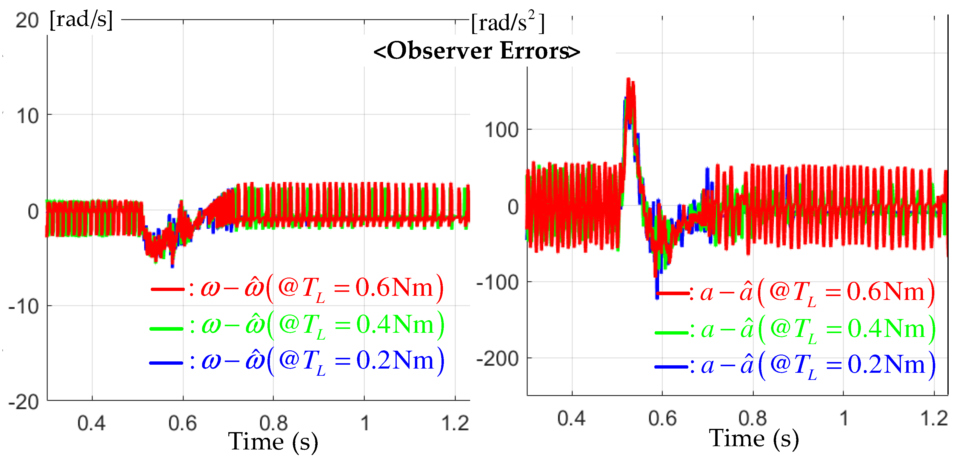
• The proposed third-order observer yields the speed and acceleration along the diagonalized error dynamics through the order reduction property without any system model information, thus specifying the nonlinear structure of the observer gain.
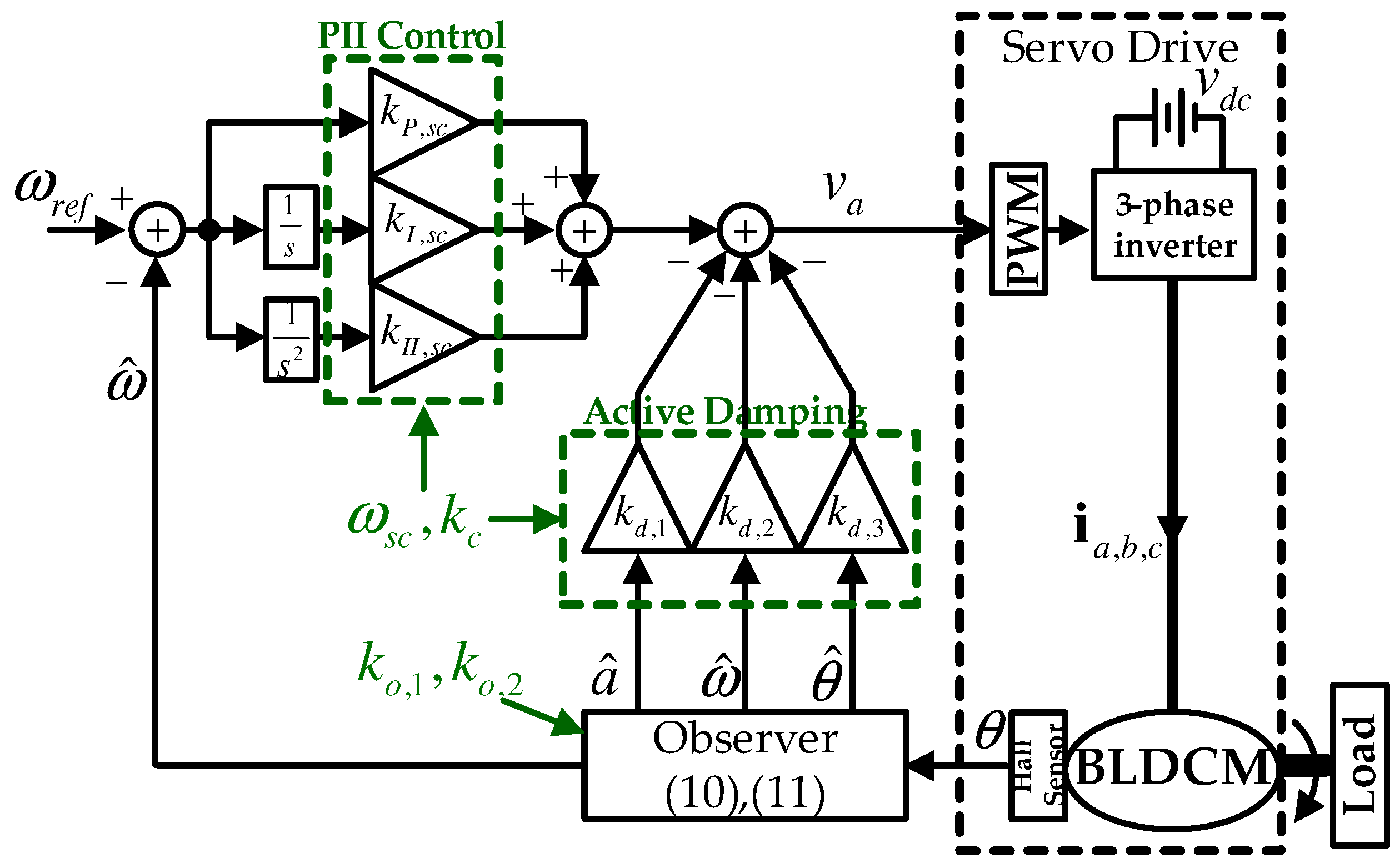
• The proposed controller preserves the simple proportional–integral–integral (PII) structure that involves the observer and active damping as the subsystems for industrial applications, thereby tuning only one of the design parameters, which determines all of the control gains for a given specification.
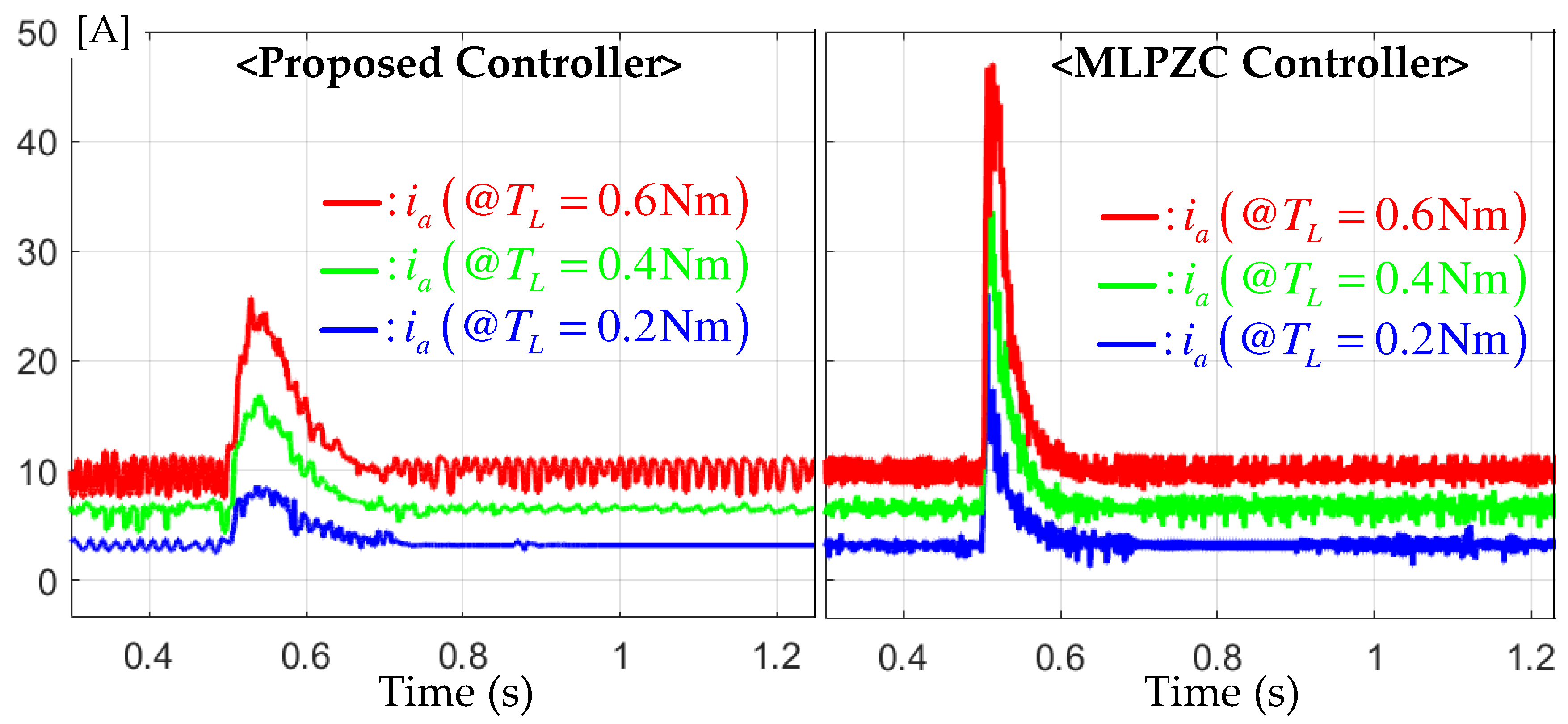
• The resultant output feedback system guarantees the desired critically damped second-order transfer function, which lowers the peak current level for transient periods.

Furthermore, a rigorous closed-loop analysis is conducted to derive beneficial closed-loop properties, which includes accomplishment of the design purpose. The experimental validation enlightens the practical contributions of the proposed technique using a hardware testbed that includes a 500 W brushless DC motor (BLDCM) and a 32-bit digital signal processor (DSP) as the servo motor and controller, respectively, under various scenarios.

2. Servo Motor Model

This work considers a DC servo motor (which includes DCM and BLDCM) to present the design purpose and result effectively and clearly; it consists of a stator, rotor (inertia : J (kgm${}^2$), and friction B (Nm/rad/s)) as the main parts. The voltage $v_a$ (V) causes an armature current $i_a$ (A) across the stator coil (inductance : L (H) and resistance : $R_a$ ($\mathrm{\Omega }$)), thereby generating the rotational torque $T_e(i_a)=k_T{i}_a$ (Nm) for some $k_T>0$. Then, the torque overwhelms the load torque $T_L$ (Nm), thus resulting in the rotor speed $\omega$ (rad/s) and position $\theta$ (rad) to lead to the back EMF ${\varphi }_b(\omega )=k_e\omega$ (V) for some $k_e>0$. These mechanisms can be described by the third-order differential equations that satisfy

$$\begin{array}{ccc}\dot{\theta }\hfill & =& \omega ,\hfill \end{array}$$

(1)

$$\begin{array}{ccc}J\dot{\omega }\hfill & =& -B\omega +T_e(i_a)-T_L,\hfill \end{array}$$

(2)

$$\begin{array}{ccc}{L}_a{\dot{i}}_a\hfill & =& -R_a{i}_a-{\varphi }_b(\omega )+v_a,\forall t\ge 0,\hfill \end{array}$$

(3)

whose uncertain parameter variations $\mathrm{\Delta }(·)$ are such that $(·)={(·)}_0+\mathrm{\Delta }(·)$, and whose mismatched uncertain disturbance $T_L$ plays a vital role in degrading the feedback system performance or causing instability, where ${(·)}_0$ represents the known nominal parameters for $(·)=J$, B, $k_T$, $L_a$, $R_a$, and $k_e$ (for instance, $J=J_0+\mathrm{\Delta }J$ with a known value $J_0$ and its uncertain variation $\mathrm{\Delta }J$). Using this concept, the two equations in (2) and (3) yielded the second-order system $v_a\mapsto \omega$ by applying the additional time derivative to (2):

$$\begin{array}{c}\hfill c_{sc,0}\ddot{\omega }=v_a+d_{\omega },\forall t\ge 0,\end{array}$$

(4)

whereby the known constant $c_{sc,0}$ and unknown time-varying signal $d_{\omega }$ are defined as $c_{sc,0}:=\frac{J_0{L}_{a,0}}{k_{T,0}}$ and $d_{\omega }:=-\mathrm{\Delta }{c}_{sc}\ddot{\omega }-B\dot{\omega }-R_a{i}_a-{\varphi }_b-{\dot{T}}_L$, respectively (where $\mathrm{\Delta }{c}_{sc}=c_{sc}-c_{sc,0}$ represents the deviation for the lumped constant defined as $c_{sc}:=\frac{J{L}_a}{k_T}$). The system representation of (4) made it possible to not only lower the system model dependence, but to also remove the requirement of the current feedback, which was then used as a basis for designing the proposed feedback system in the following section.

3. Design Purpose

When denoting the variable ${\omega }^{\ast }$ as the desired speed response, which is triggered by the reference ${\omega }_{ref}$, the Laplace transforms ${\mathrm{\Omega }}^{\ast }(s)=\mathcal{L}\left\{{\omega }^{\ast }\right\}$ and ${\mathrm{\Omega }}_{ref}(s)=\mathcal{L}\left\{{\omega }_{ref}\right\}$ define the desired transfer function for the actual feedback system ${\omega }_{ref}\mapsto \omega$ as follows:

$$\begin{array}{c}\hfill \frac{{\mathrm{\Omega }}^{\ast }(s)}{{\mathrm{\Omega }}_{ref}(s)}={(\frac{{\omega }_{sc}}{s+{\omega }_{sc}})}^2,\forall s\in \mathbb{C},\end{array}$$

(5)

which is critically damped by the multiple real pole at $-{\omega }_{sc}$ for a given specification ${\omega }_{sc}>0$ as the bandwidth ${\omega }_{sc}$ (rad/s, $f_{sc}=\frac{{\omega }_{sc}}{2\pi }$ Hz) for the transfer function (5).

The accomplishment of the exponential convergence can be expressed as follows:

$$\begin{array}{c}\hfill \underset{t\to \infty }{lim}\omega ={\omega }^{\ast },\end{array}$$

(6)

which thus permits the feedback system to ensure the desired transfer function (5). Therefore, the exponential convergence (6) was defined as the design purpose of this paper, where ${\omega }^{\ast }$ satisfies the system for the ${\mathbf{x}}^{\ast }:=\left[\begin{array}{c}{\omega }^{\ast }\\ {\dot{\omega }}^{\ast }\end{array}\right]$ (which is obtained by inverse Laplace transform for (5)). As such, this can be expressed as follows:

$$\begin{array}{c}\hfill {\dot{\mathbf{x}}}^{\ast }={\mathbf{A}}_{{\omega }_{sc}}{\mathbf{x}}^{\ast }+{\mathbf{b}}_{{\omega }_{sc}}{\omega }_{ref},{\omega }^{\ast }={\mathbf{c}}_{{\omega }_{sc}}^T{\mathbf{x}}^{\ast },\forall t\ge 0,\end{array}$$

(7)

which involve matrices defined as ${\mathbf{A}}_{{\omega }_{sc}}:=\left[\begin{array}{cc}0& 1\\ -{\omega }_{sc}^2& -2{\omega }_{sc}\end{array}\right]$, ${\mathbf{b}}_{{\omega }_{sc}}:=\left[\begin{array}{c}0\\ {\omega }_{sc}^2\end{array}\right]$, and ${\mathbf{c}}_{{\omega }_{sc}}:=\left[\begin{array}{c}1\\ 0\end{array}\right]$.

4. Implementation of the Proposed Single-Loop Feedback System

This section presents the structure and algorithm of the proposed solution for a convenient implementation. Section 4.1 and Section 4.2 provide the implementations of the proposed single-loop feedback system, which consist of an observer and controller, respectively, including a system block diagram as the conclusion of this section. Section 5.1 and Section 5.2 show how the closed-loop properties were derived so as to prove the accomplishment of the design purpose, which is described in Section 3.

4.1. Observer

The position measurement $\theta$ that is obtained from the hall sensor or rotary encoder suffers from discontinuity due to limited sensor resolution, which involves undesirable high-level noises when obtaining the speed and acceleration via the time derivative operation (e.g., $\omega =\dot{\theta }$ and $a=\dot{\omega }(=\ddot{\theta })$). This challenge can be addressed by adopting the conventional Luenberger observer, which requires exact model information (model dependency). To remove the model dependency, this work adopts the general identity for any function yielding $a=a_0+\mathrm{\Delta }a$ for ${\dot{a}}_0=0$ (e.g., DC offset) and $\mathrm{\Delta }\dot{a}\ne 0$ (e.g., AC variations).

With the facts that $\dot{\theta }=\omega$ and $\dot{\omega }=a$, this leads to the observable system for $\mathit{\theta }:=\left[\begin{array}{c}\theta \\ \omega \\ a\end{array}\right]$:

$$\begin{array}{ccc}\hfill \dot{\mathit{\theta }}& =& {\mathbf{A}}_{\mathit{\theta }}\theta +{\mathbf{b}}_{\theta }{f}_a,\hfill \end{array}$$

(8)

$$\begin{array}{ccc}\hfill \theta & =& {\mathbf{c}}_{\theta }^T\mathit{\theta },\forall t\ge 0,\hfill \end{array}$$

(9)

where ${\mathbf{A}}_{\theta }:=\left[\begin{array}{ccc}0& 1& 0\\ 0& 0& 1\\ 0& 0& 0\end{array}\right]$, ${\mathbf{b}}_{\theta }:=\left[\begin{array}{c}0\\ 0\\ 1\end{array}\right]$, ${\mathbf{c}}_{\theta }:=\left[\begin{array}{c}1\\ 0\\ 0\end{array}\right]$, (unknown disturbance) $f_a:=\mathrm{\Delta }\dot{a}$, and $|f_a|\le {\overline{f}}_a$, $\forall t\ge 0$. The proposed observer estimates the speed and acceleration by updating $\widehat{\mathit{\theta }}:=\left[\begin{array}{c}\widehat{\theta }\\ \widehat{\omega }\\ \widehat{a}\end{array}\right]$ such that

$$\begin{array}{ccc}\hfill \dot{\widehat{\mathit{\theta }}}& =& {\mathbf{A}}_{\theta }\widehat{\mathit{\theta }}+{\mathbf{l}}_{\theta }(\theta -\widehat{\theta }),\hfill \end{array}$$

(10)

$$\begin{array}{ccc}\hfill \widehat{\theta }& =& {\mathbf{c}}_{\theta }^T\widehat{\mathit{\theta }},\forall t\ge 0,\hfill \end{array}$$

(11)

thereby equipping the gain ${\mathbf{l}}_{\theta }=\left[\begin{array}{c}{l}_{\theta ,1}\\ l_{\theta ,2}\\ l_{\theta ,3}\end{array}\right]$, which is defined as

$$\begin{array}{c}\hfill l_{\theta ,1}=k_{o,1}+2k_{o,2},l_{\theta ,2}=2k_{o,1}{k}_{o,2}+k_{o,2}^2,l_{\theta ,3}=k_{o,1}{k}_{o,2}^2,\end{array}$$

(12)

whose nonlinear structure for the two design parameters $k_{o,1}>0$ (for estimation error convergence) and $k_{o,2}>0$ (for disturbance attenuation level) corresponds to a main feature of this study.

Remark 1. 

The proposed observer of (10) and (11) equipping the gain (12) yields the diagonal system for ${\mathit{e}}_{\theta }:=\mathit{\theta }-\widehat{\mathit{\theta }}(=\left[\begin{array}{c}{e}_{\theta }\\ e_{\omega }\\ e_a\end{array}\right]=\left[\begin{array}{c}\theta -\widehat{\theta }\\ \omega -\widehat{\omega }\\ a-\widehat{a}\end{array}\right])$ as follows:

$$\begin{array}{c}\hfill {\dot{\mathit{e}}}_{\theta }=-k_{o,1}{\mathit{e}}_{\theta },\forall t\ge 0,\end{array}$$

which, due to the nonlinear structure of the observer gain ${\mathit{l}}_{\theta }$, constrain $k_{o,2}$ into some admissible range. Therefore, the proposed observer requires a simple repetitive tuning process for only one scalar design parameter $k_{o,2}$ for the desired convergence rate $k_{o,1}$. Thus, unlike a conventional observer, which involves complicated matrix calculations for the tuning process, this is a practical merit of this paper. Section 5 includes the detailed property with the proof.

4.2. Controller

An open-loop system (4) yields another system for ${\mathbf{v}}_a\mapsto \widehat{\omega }$ via the identity $c_{sc,0}\widehat{\omega }=c_{sc,0}\omega +c_{sc,0}{e}_{\omega }$, which can be expressed as follows:

$$\begin{array}{c}\hfill c_{sc,0}\ddot{\widehat{\omega }}=v_a+d_{\omega }+{\mathit{c}}_1^T{\ddot{\mathit{e}}}_{\theta },\forall t\ge 0,\end{array}$$

(13)

where ${\mathbf{c}}_1:=\left[\begin{array}{c}0\\ c_{sc,0}\\ 0\end{array}\right]$. The proposed algorithm for $v_a$, driven by the error $\tilde{\omega }:={\omega }_{ref}-\widehat{\omega }$, is given by incorporating the observer state $\mathit{\theta }$ in the form of PII control as follows:

$$\begin{array}{c}\hfill v_a=-k_{d,1}\widehat{a}-k_{d,2}\widehat{\omega }-k_{d,3}\widehat{\theta }+k_{P,sc}\tilde{\omega }+k_{I,sc}{\int }_0^t\tilde{\omega }d\tau +k_{II,sc}{\int }_0^t{\int }_0^t\tilde{\omega }d{\tau }^2,\forall t\ge 0,\end{array}$$

(14)

whereby the active damping gains are equipped as

$$\begin{array}{c}\hfill k_{d,1}:=2({\omega }_{sc}{c}_{sc,0}+\sqrt{c_{sc,0}}{k}_c),k_{d,2}:=4k_c\sqrt{c_{sc,0}}{\omega }_{sc}+k_c^2,k_{d,3}:=2k_c^2{\omega }_{sc},\end{array}$$

(15)

and the PII gains are

$$\begin{array}{c}\hfill k_{P,sc}:=c_{sc,0}{\omega }_{sc}^2,k_{I,sc}:=2k_c\sqrt{c_{sc,0}}{\omega }_{sc}^2,k_{II,sc}:=k_c^2{\omega }_{sc}^2,\end{array}$$

(16)

whose nonlinear structure with respect to the design parameter $k_c>0$ for a given specification ${\omega }_{sc}>0$ corresponds to a main feature of this work.

Remark 2. 

The resultant system controlled by the proposed controller is obtained by substituting (14) into (13) such that

$$\begin{array}{ccc}\hfill c_{sc,0}\stackrel{⃜}{\widehat{\omega }}& =& -k_{d,1}\stackrel{⃛}{\widehat{\omega }}-k_{d,2}\ddot{\widehat{\omega }}-k_{d,3}\dot{\widehat{\omega }}+k_{P,sc}\ddot{\tilde{\omega }}+k_{I,sc}\dot{\tilde{\omega }}+k_{II,sc}\tilde{\omega }+{\ddot{d}}_{\omega }\hfill \\ & & +{\mathit{c}}_1^T{\stackrel{⃜}{\mathit{e}}}_{\theta }+{\mathit{c}}_2^T{\ddot{\mathit{e}}}_{\theta }+{\mathit{c}}_3^T{\dot{\mathit{e}}}_{\theta },\forall t\ge 0,\hfill \end{array}$$

(17)

where ${\mathit{c}}_2:=\left[\begin{array}{c}{k}_{d,1}{l}_{\theta ,2}\\ 0\\ 0\end{array}\right]$ and ${\mathit{c}}_3:=\left[\begin{array}{c}-k_{d,2}{l}_{\theta ,1}\\ 0\\ 0\end{array}\right]$. At this time, it is questionable that the complicated fourth-order system (17), which includes the six gains $k_{d,1}$, $k_{d,2}$, $k_{d,3}$, $k_{P,sc}$, $k_{I,sc}$, and $k_{II,sc}$, ensures exponential convergence (6). Section 5 systematically addresses this issue by further analyzing the closed-loop dynamics (17). Figure 1 visualizes the proposed feedback system structure as the block diagram by showing the simple output feedback structure and convenient tuning tasks via the four design parameters of $k_{o,1}$, $k_{o,2}$, ${\omega }_{sc}$, and $k_c$.

5. Convergence Analysis Results

The main objective of this section is to prove the accomplishment of the design purpose (6) through the analysis of the controlled system of (17) with the gains of (15) and (16), as well as the observer of (10) and (11) with the gains of (12). Section 5.1 starts from the analysis of the observer dynamics, which makes the control loop analysis convenient, as shown in Section 5.2.

5.1. Observer

This subsection proves the statement of Remark 1. To this end, Lemma 1 derives the output error dynamics as the perturbed first-order system through the combination of the systems of (10) and (11), as well as the nonlinear structure of the observer gain of (12), which invokes the order reduction property.

Lemma 1. 

The proposed observer of (10) and (11) drives its output error $e_{\theta }$ to be governed by

$$\begin{array}{c}\hfill {\dot{e}}_{\theta }=-k_{o,1}{e}_{\theta }+{\mathit{e}}_1^T{\mathit{p}}_{\theta },\end{array}$$

(18)

with ${\mathit{p}}_{\theta }(=\left[\begin{array}{c}{p}_{\theta ,1}\\ p_{\theta ,2}\end{array}\right])$ solving the perturbed system by $f_a$ as follows:

$$\begin{array}{c}\hfill {\dot{\mathit{p}}}_{\theta }={\mathit{A}}_{p_{\theta }}{\mathit{p}}_{\theta }+{\mathit{e}}_2{f}_a,\forall t\ge 0,\end{array}$$

(19)

where the matrices are defined as ${\mathit{A}}_{p_{\theta }}:=\left[\begin{array}{cc}-k_{o,2}& 1\\ 0& -k_{o,2}\end{array}\right]$, ${\mathit{e}}_1:=\left[\begin{array}{c}1\\ 0\end{array}\right]$, and ${\mathit{e}}_2:=\left[\begin{array}{c}0\\ 1\end{array}\right]$.

Proof. 

The error ${\mathbf{e}}_{\theta }$ satisfies (8) and (10) such that

$$\begin{array}{ccc}\hfill {\dot{\mathbf{e}}}_{\theta }& =& {\mathbf{A}}_{\theta ,l}{\mathbf{e}}_{\theta }+{\mathbf{b}}_{r}r+{\mathbf{b}}_{\theta }{f}_a,\hfill \end{array}$$

(20)

$$\begin{array}{ccc}\hfill e_{\theta }& =& {\mathbf{c}}_{\theta }^T{\mathbf{e}}_{\theta },\forall t\ge 0,\hfill \end{array}$$

(21)

with the matrices defined as ${\mathbf{A}}_{\theta ,l}:={\mathbf{A}}_{\theta }-{\mathbf{l}}_{\theta }{\mathbf{c}}_{\theta }^T(=\left[\begin{array}{ccc}-(k_{o,1}+2k_{o,2})& 1& 0\\ -(2k_{o,1}{k}_{o,2}+k_{o,2}^2)& 0& 1\\ -k_{o,1}{k}_{o,2}^2& 0& 0\end{array}\right])$, ${\mathbf{b}}_r:=\left[\begin{array}{c}{k}_{o,1}\\ 2k_{o,1}{k}_{o,2}\\ k_{o,1}{k}_{o,2}^2\end{array}\right]$, and $r:=0$, whose Laplace transforms (e.g., $E_{\theta }(s)=\mathcal{L}\left\{e_{\theta }\right\}$, $R(s)=\mathcal{L}\left\{r\right\}$, and $F_a(s)=\mathcal{L}\left\{f_a\right\}$) yield that

$$\begin{array}{c}\hfill E_{\theta }(s)={\mathbf{c}}_{\theta }^T{(s{\mathbf{I}}_{3\times 3}-{\mathbf{A}}_{\theta ,l})}^{-1}{\mathbf{b}}_{r}R(s)+{\mathbf{c}}_{\theta }^T{(s{\mathbf{I}}_{3\times 3}-{\mathbf{A}}_{\theta ,l})}^{-1}{\mathbf{b}}_{\theta }{F}_a(s),\forall s\in \mathbb{C}.\end{array}$$

(22)

The pair of $({\mathbf{A}}_{\theta ,l},{\mathbf{b}}_r)$ derive interesting calculation results for the first term of the right-hand side (RHS) of (22) as

$$\begin{array}{c}\hfill {\mathbf{c}}_{\theta }^T{(s{\mathbf{I}}_{3\times 3}-{\mathbf{A}}_{\theta ,l})}^{-1}{\mathbf{b}}_r=\frac{k_{o,1}{(s+k_{o,2})}^2}{(s+k_{o,1}){(s+k_{o,2})}^2}=\frac{k_{o,1}}{s+k_{o,1}}.\end{array}$$

(23)

The second term of the RHS is obtained as

$$\begin{array}{c}\hfill {\mathbf{c}}_{\theta }^T{(s{\mathbf{I}}_{3\times 3}-{\mathbf{A}}_{\theta ,l})}^{-1}{\mathbf{b}}_{\theta }=\frac{1}{(s+k_{o,1}){(s+k_{o,2})}^2},\end{array}$$

(24)

which follows from (22) that

$$\begin{array}{c}\hfill (s+k_{o,1})E_{\theta }(s)=\frac{1}{{(s+k_{o,2})}^2}{F}_a(s),\forall s\in \mathbb{C}.\end{array}$$

(25)

Therefore, the definitions $P_{\theta ,1}(s):=\frac{1}{s+k_{o,2}}{P}_{\theta ,2}(s)$ and $P_{\theta ,2}(s):=\frac{1}{s+k_{o,2}}{F}_a(s)$ confirm the result of this lemma by $e_{\theta }={\mathcal{L}}^{-1}\left\{E_{\theta }(s)\right\}$, $p_{\theta ,1}={\mathcal{L}}^{-1}\left\{P_{\theta ,1}(s)\right\}$, $p_{\theta ,2}={\mathcal{L}}^{-1}\left\{P_{\theta ,2}(s)\right\}$, and $f_a={\mathcal{L}}^{-1}\left\{F_a(s)\right\}$. □

Lemma 2 provides the essential property for the diagonalized error dynamics (stated in Remark 1) with the feasible tuning range of $k_{o,2}>0$ via the result of Lemma 1.

Lemma 2. 

The proposed observer of (10) and (11) ensures

$$\begin{array}{c}\hfill \underset{t\to \infty }{lim}{e}_{\theta }=e_{\theta }^{\ast }\end{array}$$

(26)

which exponentially, with $e_{\theta }^{\ast }$, satisfies the following system:

$$\begin{array}{c}\hfill {\dot{e}}_{\theta }^{\ast }=-k_{o,1}{e}_{\theta }^{\ast },\forall t\ge 0,\end{array}$$

(27)

for any $k_{o,2}$ such that $\frac{2{\overline{f}}_a}{k_{o,2}}\approx 0$.

Proof. 

It follows from the definitions of ${\delta }_{\theta }:=\left[\begin{array}{c}{\delta }_{\theta }\\ p_{\theta ,1}\end{array}\right]$ and ${\delta }_{\theta }:=e_{\theta }^{\ast }-e_{\theta }$, as well as the systems (18) and (19) that

$$\begin{array}{c}\hfill {\dot{\delta }}_{\theta }={\mathbf{A}}_{{\delta }_{\theta }}{\delta }_{\theta }+{\mathit{e}}_2{p}_{\theta ,2},\forall t\ge 0,\end{array}$$

(28)

where the matrices are defined as ${\mathbf{A}}_{{\delta }_{\theta }}:=\left[\begin{array}{cc}-k_{o,1}& -1\\ 0& -k_{o,2}\end{array}\right]$ and ${\mathit{e}}_2=\left[\begin{array}{c}0\\ 1\end{array}\right]$. The conditions $k_{o,1}>0$ and $k_{o,2}>0$ ensure the solvability of the equation ${\mathbf{A}}_{{\delta }_{\theta }}^T{\mathbf{P}}_{{\delta }_{\theta }}+{\mathbf{P}}_{{\delta }_{\theta }}{\mathbf{A}}_{{\delta }_{\theta }}=-{\mathbf{I}}_{2\times 2}$ with respect to a unique solution ${\mathbf{P}}_{{\delta }_{\theta }}={\mathbf{P}}_{{\delta }_{\theta }}^T>{\mathbf{0}}_{2\times 2}$, which yields for the positive definite function $V_o:=\frac{1}{2}{\delta }_{\theta }^T{\mathbf{P}}_{{\delta }_{\theta }}{\delta }_{\theta }+\frac{{\alpha }_o}{2}{p}_{\theta ,2}^2$ with ${\alpha }_o>0$ that ${\dot{V}}_o={\delta }_{\theta }^T{\mathbf{P}}_{{\delta }_{\theta }}({\mathbf{A}}_{{\delta }_{\theta }}{\delta }_{\theta }+{\mathit{e}}_2{p}_{\theta ,2})+{\alpha }_o{p}_{\theta ,2}(-k_{o,2}{p}_{\theta ,2}+f_a)$ when using the second row of (19) and (28). The fact ${\mathbf{x}}^T\mathbf{y}\le \frac{ϵ}{2}{\parallel \mathbf{x}\parallel }^2+\frac{1}{2ϵ}{\parallel \mathbf{y}\parallel }^2$, $\forall \mathbf{x},\mathbf{y}\in {\mathbb{R}}^n$, $\forall ϵ>0$ (Young’s inequality) leads to the inequality ${\dot{V}}_o\le -\frac{1}{4}\parallel {\delta }_{\theta }{\parallel }^2-(\frac{{\alpha }_o{k}_{o,2}}{2}-\parallel {\mathbf{P}}_{{\delta }_{\theta }}{\parallel }^2)p_{\theta ,2}^2+{\alpha }_o{p}_{\theta ,2}(-\frac{k_{o,2}}{2}{p}_{\theta ,2}+f_a)$ results in

$$\begin{array}{c}\hfill {\dot{V}}_o\le -{\gamma }_o{V}_o,\forall t\ge 0,\forall \left|p_{\theta }\right|\ge \frac{2{\overline{f}}_a}{k_{o,2}},\end{array}$$

(29)

whereby the removal of the indefinite terms by the choice ${\alpha }_o=\frac{2}{k_{o,2}}(\parallel {\mathbf{P}}_{{\delta }_{\theta }}{\parallel }^2+\frac{1}{2})$ is ${\gamma }_o:=min\{\frac{1}{2{\lambda }_{min}({\mathbf{P}}_{{\delta }_{\theta }})},\frac{1}{{\alpha }_o}\}$, thus validating the proof of this lemma. □

The property (26) as the result of Lemma 2 means that one can infer that ${\dot{e}}_{\theta }=-k_{o,1}{e}_{\theta }$ after a short transient period. Through this, the chain reasoning process is derived using the first row of (10) such that ${\ddot{e}}_{\theta }=-k_{o,1}{\dot{e}}_{\theta }\iff (\dot{\omega }-\ddot{\widehat{\theta }})=-k_{o,1}(\omega -\dot{\widehat{\theta }})\iff (\dot{\omega }-(l_{\theta ,1}{\dot{e}}_{\theta }+\dot{\widehat{\omega }}))=-k_{o,1}(\omega -(l_{\theta ,1}{e}_{\theta }+\widehat{\omega }))\iff {\dot{e}}_{\omega }+l_{\theta ,1}{k}_{o,1}{e}_{\theta }=-k_{o,1}{e}_{\omega }+l_{\theta ,1}{k}_{o,1}{e}_{\theta }$. Thus, it holds that ${\dot{e}}_{\omega }=-k_{o,1}{e}_{\omega }$ is from ${\dot{e}}_{\theta }=-k_{o,1}{e}_{\theta }$, thereby showing that ${\dot{e}}_a=-k_{o,1}{e}_a$ is obtained via the same process detailed above when using the second row of (11). Therefore, this subsection concludes that

$$\begin{array}{c}\hfill {\dot{\mathbf{e}}}_{\theta }=-k_{o,1}{\mathbf{e}}_{\theta },\forall t\ge 0,\end{array}$$

(30)

as the proof of Remark 1.

5.2. Control Loop

Before proceeding with the proof of the accomplishment of the design purpose (6), Lemma 3 derives the controlled speed dynamics as a perturbed second-order system through a further analysis of the system (17) with the nonlinear structure of control gains (15) and (16), thus invoking the order reduction property.

Lemma 3. 

The proposed PII controller of (14) equipping the gains (15) and (16) drives $\widehat{\omega }$ to be governed by the second-order system:

$$\begin{array}{c}\hfill \ddot{\widehat{\omega }}+2{\omega }_{sc}\dot{\widehat{\omega }}+{\omega }_{sc}^2\widehat{\omega }={\omega }_{sc}^2{\omega }_{ref}+{\mathit{c}}_{\omega ,1}^T({\mathit{p}}_{\omega ,1}+{\mathit{p}}_{\omega ,2}),\end{array}$$

(31)

with ${\mathit{p}}_{\omega ,1}(=\left[\begin{array}{c}{p}_{\omega ,1,1}\\ p_{\omega ,1,2}\end{array}\right])$ and ${\mathit{p}}_{\omega ,2}(=\left[\begin{array}{c}{p}_{\omega ,2,1}\\ p_{\omega ,2,2}\end{array}\right])$ solving the systems as follows:

$$\begin{array}{ccc}\hfill {\dot{\mathit{p}}}_{\omega ,1}& =& {\mathit{A}}_{p_{\omega ,1}}{\mathit{p}}_{\omega ,1}+{\mathit{b}}_{p_{\omega ,1}}{f}_{\omega },\hfill \end{array}$$

(32)

$$\begin{array}{ccc}\hfill {\dot{\mathit{p}}}_{\omega ,2}& =& {\mathit{A}}_{p_{\omega ,2}}{\mathit{p}}_{\omega ,2}+{\mathit{b}}_{p_{\omega ,2}}{\mathit{e}}_{\theta },\forall t\ge 0,\hfill \end{array}$$

(33)

where the matrices are defined as ${\mathit{A}}_{p_{\omega ,1}}:=\left[\begin{array}{cc}-\frac{k_c}{\sqrt{c_{sc,0}}}& -\frac{k_c}{\sqrt{c_{sc,0}}}\\ 0& -\frac{k_c}{\sqrt{c_{sc,0}}}\end{array}\right]$, ${\mathit{A}}_{p_{\omega ,2}}=\left[\begin{array}{cc}-\frac{k_c}{\sqrt{c_{sc,0}}}& 1\\ 0& -\frac{k_c}{\sqrt{c_{sc,0}}}\end{array}\right]$, ${\mathit{c}}_{\omega ,1}=\left[\begin{array}{c}\frac{1}{c_{sc,0}}\\ 0\end{array}\right]$, ${\mathit{b}}_{p_{\omega ,1}}:=\left[\begin{array}{c}1\\ 1\end{array}\right]$, and ${\mathit{b}}_{p_{\omega ,2}}:=\left[\begin{array}{c}{\mathbf{0}}_{1\times 3}\\ {\mathit{c}}_4^T\end{array}\right]$. In addition, the disturbance $f_{\omega }$ is defined as $f_{\omega }:={\dot{d}}_{\omega }$, thereby satisfying $|f_{\omega }|\le {\overline{f}}_{\omega }$, $\forall t\ge 0$.

Proof. 

It follows from the systems (17) and (30) that $\stackrel{⃜}{\widehat{\omega }}=-\frac{k_{d,1}}{c_{sc,0}}\stackrel{⃛}{\widehat{\omega }}-\frac{k_{d,2}}{c_{sc,0}}\ddot{\widehat{\omega }}-\frac{k_{d,3}}{c_{sc,0}}\dot{\widehat{\omega }}+\frac{k_{P,sc}}{c_{sc,0}}\ddot{\tilde{\omega }}+\frac{k_{I,sc}}{c_{sc,0}}\dot{\tilde{\omega }}+\frac{k_{II,sc}}{c_{sc,0}}\tilde{\omega }+\frac{1}{c_{sc,0}}{\ddot{d}}_{\omega }+\frac{1}{c_{sc,0}}{\mathbf{c}}_4^T{\mathbf{e}}_{\theta }$, where ${\mathbf{c}}_4:=k_{o,1}^4{\mathbf{c}}_1+k_{o,1}^2{\mathbf{c}}_2-k_{o,1}{\mathbf{c}}_3$, $\forall t\ge 0$. Defining signals such that $z_2:={\int }_0^t(-k_{d,2}\widehat{\omega }+k_{P,sc}\tilde{\omega }+z_2+d_{\omega ,e})d\tau$, $z_3:={\int }_0^t(-k_{d,3}\widehat{\omega }+k_{I,sc}\tilde{\omega }+z_3)d\tau$, $z_4:=k_{II,sc}{\int }_0^t\tilde{\omega }d\tau$, and $d_{\omega ,e}:=d_{\omega }+{\mathbf{c}}_4^T{\int }_0^t{\int }_0^t{\mathbf{e}}_{\theta }d{\tau }^2$ for the vector ${\mathbf{z}}_{\omega }:={\left[\begin{array}{cccc}\widehat{\omega }& z_2& z_3& z_4\end{array}\right]}^T$ yield another expression for the system (17) as

$$\begin{array}{ccc}\hfill {\dot{\mathbf{z}}}_{\omega }& =& {\mathbf{A}}_{z_{\omega }}{\mathbf{z}}_{\omega }+{\mathbf{b}}_{z_{\omega },r}{\omega }_{ref}+{\mathbf{b}}_{z_{\omega },d}{d}_{\omega ,e},\hfill \end{array}$$

(34)

$$\begin{array}{ccc}\hfill \widehat{\omega }& =& {\mathbf{c}}_{z_{\omega }}^T{\mathbf{z}}_{\omega },\forall t\ge 0,\hfill \end{array}$$

(35)

with the matrices defined as ${\mathbf{A}}_{z_{\omega }}:=\left[\begin{array}{cccc}-\frac{2({\omega }_{sc}{c}_{sc,0}+\sqrt{c_{sc,0}}{k}_c)}{c_{sc,0}}& \frac{1}{c_{sc,0}}& 0& 0\\ -(4k_c\sqrt{c_{sc,0}}{\omega }_{sc}+k_c^2+c_{sc,0}{\omega }_{sc}^2)& 0& 1& 0\\ -(2k_c^2{\omega }_{sc}+2k_c\sqrt{c_{sc,0}}{\omega }_{sc}^2)& 0& 0& 1\\ -k_c^2{\omega }_{sc}^2& 0& 0& 0\end{array}\right]$, ${\mathbf{b}}_{z_{\omega },r}:=\left[\begin{array}{c}0\\ c_{sc,0}{\omega }_{sc}^2\\ 2k_c\sqrt{c_{sc,0}}{\omega }_{sc}^2\\ k_c^2{\omega }_{sc}^2\end{array}\right]$, ${\mathbf{b}}_{z_{\omega },d}:=\left[\begin{array}{c}0\\ 1\\ 0\\ 0\end{array}\right]$, and ${\mathbf{c}}_{z_{\omega }}:=\left[\begin{array}{c}1\\ 0\\ 0\\ 0\end{array}\right]$. The variables $\widehat{\mathrm{\Omega }}(s)=\mathcal{L}\left\{\widehat{\omega }\right\}$, ${\mathrm{\Omega }}_{ref}(s)=\mathcal{L}\left\{{\omega }_{ref}\right\}$, and $D_{\omega ,e}(s)=\mathcal{L}\left\{d_{\omega ,e}\right\}(=D_{\omega }(s)+\frac{1}{s^2}{\mathbf{c}}_4^T{\mathbf{E}}_{\theta }(s))$ derive an equivalent expression for the system, consisting of (34) and (35) as

$$\begin{array}{c}\hfill \widehat{\mathrm{\Omega }}(s)={\mathbf{c}}_{z_{\omega }}^T(s{\mathbf{I}}_{4\times 4}-{\mathbf{A}}_{z_{\omega }}){\mathbf{b}}_{z_{\omega },r}{\mathrm{\Omega }}_{ref}(s)+{\mathbf{c}}_{z_{\omega }}^T(s{\mathbf{I}}_{4\times 4}-{\mathbf{A}}_{z_{\omega }}){\mathbf{b}}_{z_{\omega },d}{D}_{\omega ,e}(s),\forall s\in \mathbb{C}.\end{array}$$

(36)

The pair (${\mathbf{A}}_{z_{\omega }}$, ${\mathbf{b}}_{z_{\omega },r}$) derive an interesting calculation result for the first term of the RHS of (36) as

$$\begin{array}{c}\hfill {\mathbf{c}}_{z_{\omega }}^T(s{\mathbf{I}}_{4\times 4}-{\mathbf{A}}_{z_{\omega }}){\mathbf{b}}_{z_{\omega },r}=\frac{{\omega }_{sc}^2{(\sqrt{c_{sc,0}}s+k_c)}^2}{{(s+{\omega }_{sc})}^2{(\sqrt{c_{sc,0}}s+k_c)}^2}={(\frac{{\omega }_{sc}}{s+{\omega }_{sc}})}^2,\end{array}$$

(37)

and the second term of the RHS is obtained as

$$\begin{array}{c}\hfill {\mathbf{c}}_{z_{\omega }}^T(s{\mathbf{I}}_{4\times 4}-{\mathbf{A}}_{z_{\omega }}){\mathbf{b}}_{z_{\omega },d}=\frac{s^2}{{(s+{\omega }_{sc})}^2{(\sqrt{c_{sc,0}}s+k_c)}^2},\end{array}$$

(38)

which follows from (36) that

$$\begin{array}{c}\hfill {(s+{\omega }_{sc})}^2\widehat{\mathrm{\Omega }}(s)={\omega }_{sc}^2{\mathrm{\Omega }}_{ref}(s)+\frac{1}{c_{sc,0}}{(\frac{s}{s+\frac{k_c}{\sqrt{c_{sc,0}}}})}^2{D}_{\omega }(s)+\frac{1}{c_{sc,0}}\frac{1}{{(s+\frac{k_c}{\sqrt{c_{sc,0}}})}^2}{\mathbf{c}}_4^T{\mathbf{e}}_{\theta },\end{array}$$

(39)

$\forall s\in \mathbb{C}$. Therefore, the definitions $P_{\omega ,1,1}(s)=(1-\frac{\frac{k_c}{\sqrt{c_{sc,0}}}}{s+\frac{k_c}{\sqrt{c_{sc,0}}}})P_{\omega ,1,2}(s)$, $P_{\omega ,1,2}(s)=(1-\frac{\frac{k_c}{\sqrt{c_{sc,0}}}}{s+\frac{k_c}{\sqrt{c_{sc,0}}}})D_{\omega }(s)$, $P_{\omega ,2,1}(s)=(\frac{1}{s+\frac{k_c}{{\sqrt{c}}_{sc,0}}})P_{\omega ,2,2}(s)$, and $P_{\omega ,2,2}(s)=(\frac{1}{s+\frac{k_c}{{\sqrt{c}}_{sc,0}}}){\mathbf{c}}_4^T{\mathbf{E}}_{\theta }(s)$ complete the proof by $p_{\omega ,i}={\mathcal{L}}^{-1}\left\{P_{\omega ,i}(s)\right\}$ and $p_{\omega ,2,i}={\mathcal{L}}^{-1}\left\{P_{\omega ,2,i}(s)\right\}$, $i=1,2$, with ${\mathbf{p}}_{\omega ,1}={\left[\begin{array}{cc}{p}_{\omega ,1,1}& p_{\omega ,1,2}\end{array}\right]}^T$ and ${\mathbf{p}}_{\omega ,2}={\left[\begin{array}{cc}{p}_{\omega ,2,1}& p_{\omega ,2,2}\end{array}\right]}^T$. □

In conclusion, Theorem 1 ends this section by proving the accomplishment of the design objective (6) with the specification of the tuning range of $k_c>0$ when using the results of Lemma 3 and the diagonalized observer error dynamics of (30).

Theorem 1. 

The proposed controller depicted in Figure 1 establishes the design purpose (6) (e.g., ${lim}_{t\to \infty }\omega ={\omega }^{\ast }$ exponentially) for any $k_c$ such that $\frac{2\sqrt{c_{sc,0}}{\overline{f}}_{\omega }}{k_c}\approx 0$.

Proof. 

The vector $\mathbf{x}$ defined as $\mathbf{x}:=\left[\begin{array}{c}\widehat{\omega }\\ \dot{\widehat{\omega }}\end{array}\right]$ yields the vector form for the system (31) as $\dot{\mathbf{x}}={\mathbf{A}}_{{\omega }_{sc}}\mathbf{x}+{\mathbf{b}}_{{\omega }_{sc}}{\omega }_{ref}+{\mathbf{e}}_2(\frac{1}{c_{sc,0}}{p}_{\omega ,1,1}+{\mathbf{c}}_{\omega ,1}^T{\mathbf{p}}_{\omega ,2})$. This leads to another system for deviation, which is defined as ${\delta }_{\omega }:={\mathbf{x}}^{\ast }-\mathbf{x}$ together with the two systems of (7) and (32):

$$\begin{array}{ccc}\hfill {\dot{\delta }}_{\omega }& =& {\mathbf{A}}_{{\delta }_{\omega }}{\delta }_{\omega }+{\mathbf{b}}_{{\delta }_{\omega },1}{p}_{\omega ,1,1}+{\mathbf{B}}_{{\delta }_{\omega },2}{\mathbf{p}}_{\omega ,2},\hfill \end{array}$$

(40)

$$\begin{array}{ccc}\hfill {\dot{p}}_{\omega ,1,1}& =& -\frac{k_c}{\sqrt{c_{sc,0}}}{p}_{\omega ,1,1}-\frac{k_c}{\sqrt{c_{sc,0}}}{p}_{\omega ,1,2}+f_{\omega },\hfill \end{array}$$

(41)

$$\begin{array}{ccc}\hfill {\dot{p}}_{\omega ,1,2}& =& -\frac{k_c}{\sqrt{c_{sc,0}}}{p}_{\omega ,1,2}+f_{\omega },\forall t\ge 0,\hfill \end{array}$$

(42)

where ${\mathbf{A}}_{{\delta }_{\omega }}={\mathbf{A}}_{{\omega }_{sc}}$, ${\mathbf{b}}_{{\delta }_{\omega },1}:=-\frac{1}{c_{sc,0}}{\mathbf{e}}_2$, and ${\mathbf{B}}_{{\delta }_{\omega },2}:=-{\mathbf{e}}_2{\mathbf{c}}_{\omega ,1}^T$. The conditions ${\omega }_{sc}>0$, $k_c>0$ and $c_{sc,0}>0$ ensure the solvability of the equation ${\mathbf{A}}_{{\delta }_{\omega }}^T{\mathbf{P}}_{{\delta }_{\omega }}+{\mathbf{P}}_{{\delta }_{\omega }}{\mathbf{A}}_{{\delta }_{\omega }}=-{\mathbf{I}}_{2\times 2}$ and ${\mathbf{A}}_{p_{\omega ,2}}^T{\mathbf{P}}_{p_{\omega ,2}}+{\mathbf{P}}_{p_{\omega ,2}}{\mathbf{A}}_{p_{\omega ,2}}=-{\mathbf{I}}_{2\times 2}$ with respect to a unique solution ${\mathbf{P}}_{{\delta }_{\omega }}={\mathbf{P}}_{{\delta }_{\omega }}^T>{\mathbf{0}}_{2\times 2}$ and ${\mathbf{P}}_{p_{\omega ,2}}={\mathbf{P}}_{p_{\omega ,2}}^T>{\mathbf{0}}_{2\times 2}$, respectively, which leads to the positive definite function $V_{sc}:=\frac{1}{2}{\delta }_{\omega }^T{\mathbf{P}}_{{\delta }_{\omega }}{\delta }_{\omega }+\frac{{\alpha }_{sc,1}}{2}{p}_{\omega ,1,1}^2+\frac{{\alpha }_{sc,2}}{2}{p}_{\omega ,1,2}^2+\frac{{\alpha }_{sc,3}}{2}{\mathbf{p}}_{\omega ,2}^T{\mathbf{P}}_{p_{\omega ,2}}{\mathbf{p}}_{\omega ,2}+\frac{{\alpha }_{sc,4}}{2}{\parallel {\mathbf{e}}_{\theta }\parallel }^2$ with ${\alpha }_{sc,i}>0$, $i=1,2,3,4$ such that ${\dot{V}}_{sc}={\delta }_{\omega }^T{\mathbf{P}}_{{\delta }_{\omega }}({\mathbf{A}}_{{\delta }_{\omega }}{\delta }_{\omega }+{\mathbf{b}}_{{\delta }_{\omega },1}{p}_{\omega ,1,1}+{\mathbf{B}}_{{\delta }_{\omega },2}{\mathbf{p}}_{\omega ,2})+{\alpha }_{sc,1}{p}_{\omega ,1,1}(-\frac{k_c}{\sqrt{c_{sc,0}}}{p}_{\omega ,1,1}-\frac{k_c}{\sqrt{c_{sc,0}}}{p}_{\omega ,1,2}+f_{\omega })+{\alpha }_{sc,2}{p}_{\omega ,1,2}(-\frac{k_c}{\sqrt{c_{sc,0}}}{p}_{\omega ,1,2}+f_{\omega })+{\alpha }_{sc,3}{\mathbf{p}}_{\omega ,2}^T{\mathbf{P}}_{p_{\omega ,2}}({\mathbf{A}}_{p_{\omega ,2}}{\mathbf{p}}_{\omega ,2}+{\mathbf{b}}_{p_{\omega ,2}}{\mathbf{e}}_{\theta })-$${\alpha }_{sc,4}{k}_{o,1}{\parallel {\mathbf{e}}_{\theta }\parallel }^2$ when using (30), (33), and (40)–(42). The Young’s inequality leads to the inequality

$$\begin{array}{ccc}\hfill {\dot{V}}_{sc}& \le & -\frac{1}{6}\parallel {\delta }_{\omega }{\parallel }^2-\frac{1}{2}(\frac{{\alpha }_{sc,1}{k}_c}{2\sqrt{c_{sc,0}}}-3\parallel {\mathbf{P}}_{{\delta }_{\omega }}{\parallel }^2\parallel {\mathbf{b}}_{{\delta }_{\omega },1}{\parallel }^2)p_{\omega ,1,1}^2-(\frac{{\alpha }_{sc,2}{k}_c}{2\sqrt{c_{sc,0}}}-\frac{{\alpha }_{sc,1}{k}_c}{\sqrt{c_{sc,0}}})p_{\omega ,1,2}^2\hfill \\ & & -\frac{1}{2}(\frac{{\alpha }_{sc,3}}{2}-3\parallel {\mathbf{P}}_{{\delta }_{\omega }}{\parallel }^2\parallel {\mathbf{B}}_{{\delta }_{\omega },2}{\parallel }^2)\parallel {\mathbf{p}}_{\omega ,2}{\parallel }^2-({\alpha }_{sc,4}{k}_{o,1}-{\alpha }_{sc,3}\parallel {\mathbf{P}}_{p_{\omega ,2}}{\parallel }^2\parallel {\mathbf{b}}_{p_{\omega ,2}}{\parallel }^2)\parallel {\mathbf{e}}_{\theta }{\parallel }^2\hfill \\ & & +{\alpha }_{sc,1}{p}_{\omega ,1,1}(-\frac{k_c}{2\sqrt{c_{sc,0}}}{p}_{\omega ,1,1}+f_{\omega })+{\alpha }_{sc,2}{p}_{\omega ,1,2}(-\frac{k_c}{2\sqrt{c_{sc,0}}}{p}_{\omega ,1,2}+f_{\omega }),\forall t\ge 0,\hfill \end{array}$$

thereby resulting in

$$\begin{array}{c}\hfill {\dot{V}}_{sc}\le -{\gamma }_{sc}{V}_{sc},\forall t\ge 0,\forall |p_{\omega ,1,1}|\ge \frac{2\sqrt{c_{sc,0}}{\overline{f}}_{\omega }}{k_c},\forall \left|p_{\omega ,1,2}\right|\ge \frac{2\sqrt{c_{sc,0}}{\overline{f}}_{\omega }}{k_c},\end{array}$$

(43)

with the removals of the indefinite terms by choices such that ${\alpha }_{sc,1}=\frac{2\sqrt{c_{sc,0}}}{k_c}(3\parallel {\mathbf{P}}_{{\delta }_{\omega }}{\parallel }^2$$\parallel {\mathbf{b}}_{{\delta }_{\omega },1}{\parallel }^2+1)$, ${\alpha }_{sc,2}=\frac{2\sqrt{c_{sc,0}}}{k_c}(\frac{{\alpha }_{sc,1}{k}_c}{\sqrt{c_{sc,0}}}+\frac{1}{2})$, ${\alpha }_{sc,3}=2(3\parallel {\mathbf{P}}_{{\delta }_{\omega }}{\parallel }^2\parallel {\mathbf{B}}_{{\delta }_{\omega ,2}}{\parallel }^2+1)$, and ${\alpha }_{sc,4}=\frac{1}{k_{o,1}}({\alpha }_{sc,3}\parallel {\mathbf{P}}_{p_{\omega ,2}}{\parallel }^2\parallel {\mathbf{b}}_{p_{\omega ,2}}{\parallel }^2+\frac{1}{2})$, where ${\gamma }_{sc}:=min\{\frac{1}{3{\lambda }_{min}({\mathbf{P}}_{{\delta }_{\omega }})},\frac{1}{{\alpha }_{sc,1}},\frac{1}{{\alpha }_{sc,2}},\frac{1}{{\alpha }_{sc,3}{\lambda }_{min}({\mathbf{P}}_{p_{\omega ,2}})},\frac{1}{{\alpha }_{sc,4}}\}$. This validates the results of this theorem. □

6. Experimental Results

6.1. Configuration for Experiments

This study constructed the dynamo-meter shown in Figure 2 (500 W BLDCM for test motor and 700 W permanent magnet synchronous motor for load motor) as the servo drive to experimentally demonstrate the advantage of the proposed solution. The commercial board (model: DRV8305; manufacture: Texas Instrument (TI)) used as the three-phase inverter operated the BLDCM by the duty command from the controller, whose DC source voltage was set to 25 V. The TI 32-bit DSP (model: LUNCHXL-F28379D) outputted the duty command from the C-programming implementation of the proposed feedback system, as shown in Figure 1, through the internal interrupt period of $0.1$ ms, which was synchronized to the control, PWM, and measurement process. The datasheet and repetitive offline identification experiments found the BLDCM parameters given by (for rotor) $J=1.7\times {10}^{-4}$, $B=2.9\times {10}^{-5}$, (for stator) $L_a=0.13\times {10}^{-3}$, $R_a=0.0785$, and (for flux) $k_T=k_e=0.068$. The controller area network constituted the real-time communication between the controller and desktop PC to collect the experimental data through MATLAB/Simulink.

The nominal values chosen as $J_0=0.8J$, $L_{a,0}=0.7L_a$, and $k_{T,0}=1.4k_T$ yielded the known lumped coefficient $c_{sc,0}=\frac{L_{a,0}{J}_0}{k_{T,0}}$, which was used for the controller to consider the model plant mismatches detailed in Section 2. As shown in Figure 1, the proposed feedback system provided the four design parameters ${\omega }_{sc}$ and $k_c$ for the controller and $k_{o,1}$ and $k_{o,2}$ for the observer, which were determined as $f_{sc}=5$ Hz (${\omega }_{sc}=2\pi 5$ rad/s), $k_c=0.5$, $k_{o,1}=50$, and $k_{o,2}=1000$, respectively.

The novel multi-loop PZC (MLPZC) controller (in [8]) was adopted to evaluate the performance improvement of the proposed technique through a comparison study. For a fair comparison, the speed loop bandwidth was set to be the same as the proposed controller under the current loop bandwidth of $f_{cc}=100$ Hz (${\omega }_{cc}=2\pi 100$ rad/s), and the remaining design parameters were tuned for the best performance.

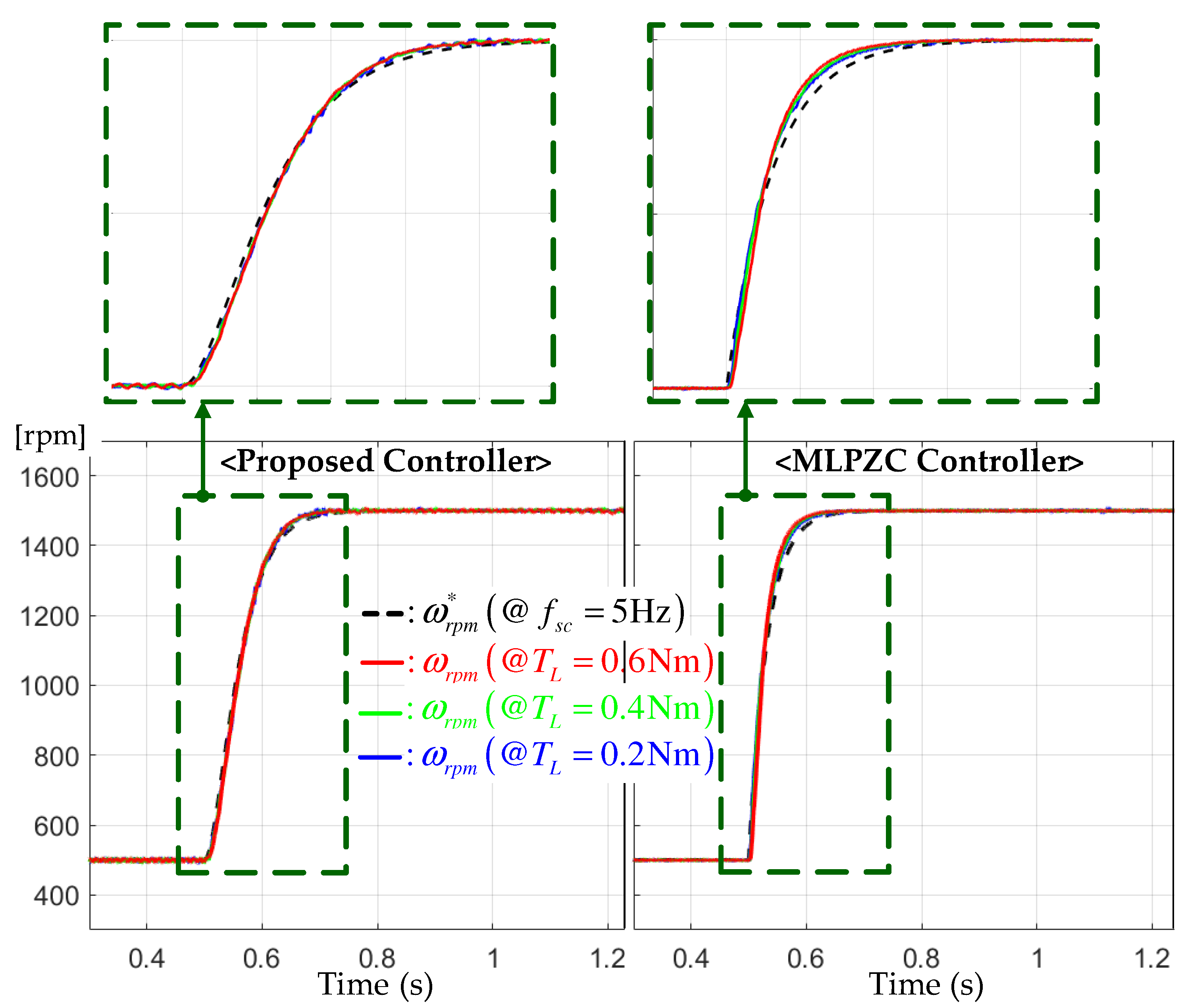
6.2. Step-Up Reference Tracking Tests

For the step-up reference from the initial value ${\omega }_{ref}=500$ to the final value 1500 rpm, this experiment was conducted three times for the different loads of $T_L=0.2$, $0.4$, and $0.6$ Nm to evaluate the speed tracking performance. Figure 3 shows the comparison results between the proposed and MLPZC controllers. Both controllers effectively assigned the desired transfer functions with the bandwidth of $f_{sc}=5$ Hz to the closed loop under different load conditions, as well as for the critical damped transfer function for the proposed controller and simple damped transfer function for the MLPZC. There were no significant performance differences between the two controllers, but the critically damping characteristic by the multiple pole at $-{\omega }_{sc}$ resulted in the improved peak current suppression capability by the proposed controller, as shown in Figure 4. This corresponded with a main advantage of this work, in practice, by adopting the second-order transfer function (5). The speed and acceleration estimation results by the proposed observer are presented in Figure 5. According to the comment of Remark 1, the proposed observer renders the speed (left side of Figure 5) and the acceleration estimation errors (right side of Figure 5) to be rapidly convergent with the zero under the same estimation error dynamics despite the different load conditions.

6.3. Constant Reference Regulation Tests

This section fixed the speed reference to ${\omega }_{ref}=1500$ rpm. The three step-up load torque increments $T_L=0.4$, $0.6$, and $0.8$ Nm from the initial setting $T_L=0.2$ Nm (e.g., $T_L:0.2\to 0.4/0.6/0.8$ Nm) were considered to evaluate the speed regulation performance under the same settings with Section 6.2. Figure 6 shows that the proposed controller’s critically damped system also improved the speed regulation performance by significantly reducing the over/undershoot level for all three different load variation scenarios. Figure 7 indicates that the proposed controller makes the current response similar to the MLPZC despite improving the speed regulation performance.

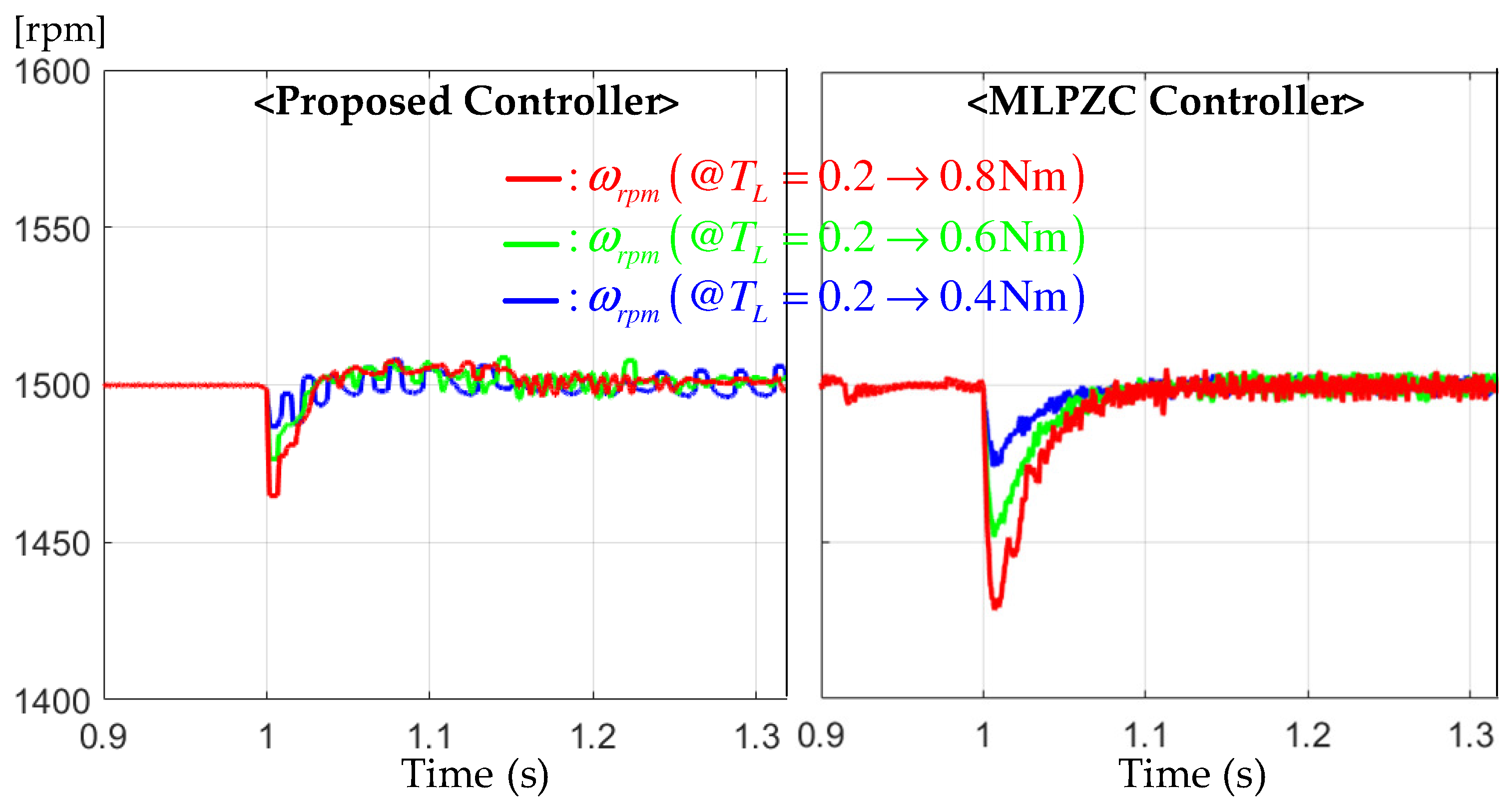
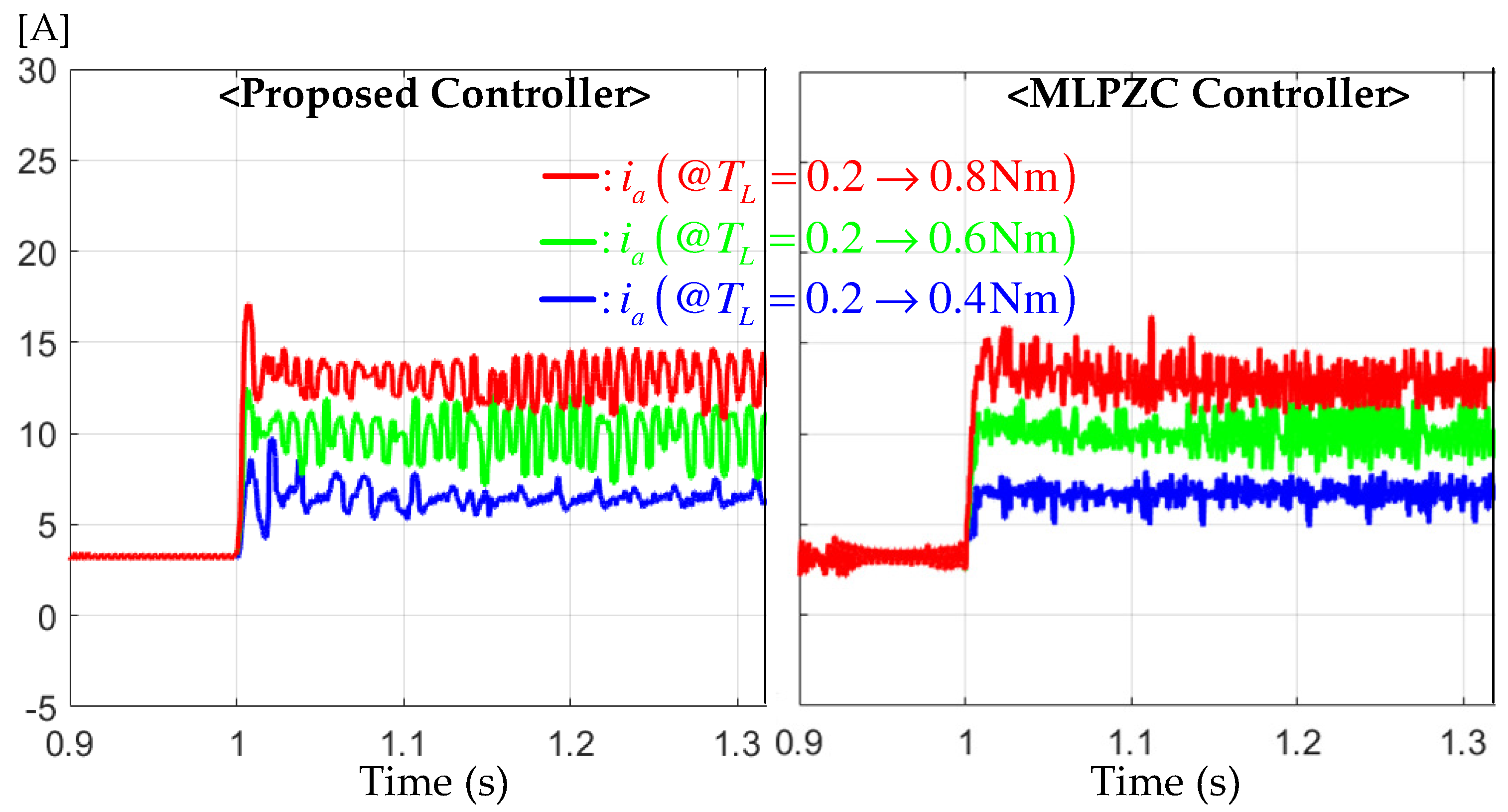
6.4. Performance Assignability Tests

This experiment was conducted to highlight the effectiveness of the result of Theorem 1. For this purpose, this section fixed the load torque to $T_L=0.2$ Nm and adopted the same step-up reference used in Section 6.2. The three increasing bandwidths of $f_{sc}=5$, 8, and 15 Hz were applied to the feedback system to observe the performance changes according to such various bandwidths. The left of Figure 8 shows that the proposed controller precisely assigned the desired transfer functions to the closed loop for each bandwidth due to the accomplishment of the design purpose by Theorem 1. Meanwhile, the right of Figure 8 presents the corresponding current responses without the peaking phenomenon due to the assigned second-order transfer function (5). With this result and the practical advantage from Section 6.2, the proposed solution would guarantee consistent performance for the actual industrial applications despite the load and user specification changes.

7. Conclusions

This paper exhibited an observer-based feedback system in a simple form for servo drive applications, which includes the model-independent speed and an acceleration observer, based on the order reduction technique. The resultant feedback system did not require the exact system model information, and its nonlinearly structured control and observer gains resulted in a desired performance that is subject to a simple or critically damped system via the PZC. Moreover, it was rigorously proved that the resultant feedback system accomplished the design purpose by specifying the feasible range of the tuning parameters. The experimental validation was also conducted to highlight the practical benefits, such as improved performance consistency and peak current attenuation, despite the simple output feedback system structure. Therefore, the proposed solution would be considered as promising actuators for industrial unmanned exploration robot and aerial vehicle applications. In the future, this result will be applied to multiple servo drive synchronization applications that adopt large-power three-phase motors with a systematical closed-loop tuning process by solving an optimization problem.

References

1. Zhu, M.; Bao, D.; Huang, X. The Design of a Tracking Controller for Flexible Ball Screw Feed System Based on Integral Sliding Mode Control with a Generalized Extended State Observer. Actuators 2023, 12, 387. [Google Scholar] [CrossRef]
2. Jayaraman, T.; Thangaraj, M. Standalone and Interconnected Analysis of an Independent Accumulator Pressure Compressibility Hydro-Pneumatic Suspension for the Four-Axle Heavy Truck. Actuators 2023, 12, 347. [Google Scholar] [CrossRef]
3. Lin, H.T.; Lee, Y.H. Implementing a Precision Pneumatic Plug Tray Seeder with High Seeding Rates for Brassicaceae Seeds via Real-Time Trajectory Tracking Control. Actuators 2023, 12, 340. [Google Scholar] [CrossRef]
4. Hou, T.; Kou, Z.; Wu, J.; Jin, T.; Su, K.; Du, B. Research on Positioning Control Strategy for a Hydraulic Support Pushing System Based on Iterative Learning. Actuators 2023, 12, 306. [Google Scholar] [CrossRef]
5. Lim, S.; Kim, S.K.; Kim, K.C. Model-Independent Observer-Based Current Sensorless Speed Servo Systems with Adaptive Feedback Gain. Actuators 2022, 11, 126. [Google Scholar] [CrossRef]
6. Agee, J.T.; Bingul, Z.; Kizir, S. Higher-order differential feedback control of a flexible-joint manipulator. J. Vib. Control 2015, 10, 1976–1986. [Google Scholar] [CrossRef]
7. Agee, J.T.; Bingul, Z.; Kizir, S. Trajectory and Vibration Control of a Single-Link Flexible-Joint Manipulator Using a Distributed Higher-Order Differential Feedback Controller. ASME J. Dyn. Syst. Meas. Control 2017, 139, 081006. [Google Scholar] [CrossRef]
8. Kim, S.K.; Ahn, C.K. Active-damping Speed Tracking Technique for Permanent Magnet Synchronous Motors with Transient Performance Boosting Mechanism. IEEE Trans. Ind. Inform. 2021, 18, 2171–2179. [Google Scholar] [CrossRef]
9. Andeescu, G.D.; Pitic, C.I.; Blaabjerg, F.; Boldea, I. Combined flux observer with signal injection enhancement for wide speed range sensorless direct torque control of IPMSM drives. IEEE Trans. Energy Convers. 2008, 23, 393–402. [Google Scholar] [CrossRef]
10. Tang, L.; Zhong, L.; Rahman, M.; Hu, Y. A novel direct torque control for interior permanent-magnet synchronous machine drive with low ripple in torque and flux - a speed-senseroless approach. IEEE Trans. Ind. Appl. 2003, 39, 1748–1756. [Google Scholar] [CrossRef]
11. Olalla, C.; Leyva, R.; Queinnec, I.; Maksimovic, D. Robust Gain-Scheduled Control of Switched-Mode DC-DC Converters. IEEE Trans. Power Electron. 2012, 27, 3006–3019. [Google Scholar] [CrossRef]
12. Sul, S.K. Control of Electric Machine Drive Systems; Wiley: Hoboken, NJ, USA, 2011; Volume 88. [Google Scholar]
13. Xu, L.; Li, Y. Distributed Adaptive Consensus Tracking Control for Second-Order Nonlinear Heterogeneous Multi-Agent Systems with Input Quantization. Machines 2023, 11, 524. [Google Scholar] [CrossRef]
14. Zhang, Y.; Zhang, M.; Fan, C.; Li, F. A Finite-Time Trajectory-Tracking Method for State-Constrained Flexible Manipulators Based on Improved Back-Stepping Control. Actuators 2022, 11, 139. [Google Scholar] [CrossRef]
15. Lin, C.Y.; Yao, W.S. Analysis and Design Multiple Layer Adaptive Kalman Filter Applied to Electro-Optical Infrared Payload Vision System. Electronics 2022, 11, 677. [Google Scholar] [CrossRef]
16. Zhang, J.; Jiang, Y.; Li, X.; Luo, H.; Yin, S.; Kaynak, O. Remaining Useful Life Prediction of Lithium-Ion Battery With Adaptive Noise Estimation and Capacity Regeneration Detection. IEEE/ASME Trans. Mechatron. 2023, 28, 632–643. [Google Scholar] [CrossRef]
17. Kim, S.K. Robust adaptive speed regulator with self-tuning law for surfaced-mounted permanent magnet synchronous motor. Control Eng. Pract. 2017, 61, 55–71. [Google Scholar] [CrossRef]
18. El-Sousy, F.F.M.; Abuhasel, K.A. Nonlinear Robust Optimal Control via Adaptive Dynamic Programming of Permanent-Magnet Linear Synchronous Motor Drive for Uncertain Two-Axis Motion Control System. IEEE Trans. Ind. Appl. 2020, 56, 1940–1952. [Google Scholar] [CrossRef]
19. Errouissi, R.; Ouhrouche, M.; Chen, W.H.; Trzynadlowski, A.M. Robust Cascaded Nonlinear Predictive Control of a Permanent Magnet Synchronous Motor With Antiwindup Compensator. IEEE Trans. Ind. Electron. 2012, 59, 3078–3088. [Google Scholar] [CrossRef]
20. Deng, W.; Yao, J.; Ma, D. Time-varying input delay compensation for nonlinear systems with additive disturbance: An output feedback approach. Int. J. Robust Nonlinear Control 2017, 28, 31–52. [Google Scholar] [CrossRef]
21. Deng, W.; Yao, J. Extended-State-Observer-Based Adaptive Control of Electrohydraulic Servomechanisms Without Velocity Measurement. IEEE/ASME Trans. Mechatron. 2020, 25, 1151–1161. [Google Scholar] [CrossRef]
22. Deng, W.; Yao, J.; Wang, Y.; Yang, X.; Chen, J. Output feedback backstepping control of hydraulic actuators with valve dynamics compensation. Mech. Syst. Signal Process. 2021, 158, 107769. [Google Scholar] [CrossRef]
23. Son, Y.I.; Kim, I.H.; Choi, D.S.; Shim, H. Robust Cascade Control of Electric Motor Drives Using Dual Reduced-Order PI Observer. IEEE Trans. Ind. Electron. 2015, 62, 3672–3682. [Google Scholar] [CrossRef]
24. Corradini, M.L.; Ippoliti, G.; Longhi, S.; Orlando, G. A Quasi-Sliding Mode Approach for Robust Control and Speed Estimation of PM Synchronous Motors. IEEE Trans. Ind. Electron. 2012, 59, 1096–1104. [Google Scholar] [CrossRef]
25. Geyer, T.; Papafotieu, G.; Morari, M. Model predictive direct torque control-part I: Concept, algorithm and analysis. IEEE Trans. Ind. Electron. 2009, 56, 1894–1905. [Google Scholar] [CrossRef]
26. Ahmed, A.A.; Koh, B.K.; Lee, Y.I. A Comparison of Finite Control Set and Continuous Control Set Model Predictive Control Schemes for Speed Control of Induction Motors. IEEE Trans. Ind. Inform. 2018, 14, 1334–1346. [Google Scholar] [CrossRef]
27. Tao, T.; Zhao, W.; Du, Y.; Cheng, Y.; Zhu, J. Simplified Fault-Tolerant Model Predictive Control for a Five-Phase Permanent-Magnet Motor With Reduced Computation Burden. IEEE Trans. Power Electron. 2020, 35, 3850–3858. [Google Scholar] [CrossRef]
28. Kim, S.K.; Kim, Y.; Ahn, C.K. Energy-Shaping Speed Controller With Time-Varying Damping Injection for Permanent-Magnet Synchronous Motors. IEEE Trans. Circuits Syst. II Express Briefs 2021, 68, 381–385. [Google Scholar] [CrossRef]
Figure 1. Block diagram of the proposed feedback system structure with four design parameters.
Actuators 13 00002 g001
Figure 2. Hardware testbed: 500 W BLDCM for test motor, PMSM for load, and 32-bit DSP for controller.
Actuators 13 00002 g002
Figure 3. Speed responses for the step-up reference tracking tests under the different loads of T L = 0.2 , 0.4 , and 0.6 Nm.
Actuators 13 00002 g003
Figure 4. Currentresponses for the step-up reference tracking tests under the different loads of T L = 0.2 , 0.4 , and 0.6 Nm.
Actuators 13 00002 g004
Figure 5. Speed and acceleration estimation errors for the step-up reference tracking tests under the different loads of T L = 0.2 , 0.4 , and 0.6 Nm.
Actuators 13 00002 g005
Figure 6. Speed responses for the constant reference regulation tests under the sudden increasing load torques of T L : 0.2 0.4 / 0.6 / 0.8 Nm.
Actuators 13 00002 g006
Figure 7. Current responses for the constant reference regulation tests under the sudden increasing load torques of T L : 0.2 0.4 / 0.6 / 0.8 Nm.
Actuators 13 00002 g007
Figure 8. Speed responses for the step-up reference tracking tests under the different bandwidths of f s c = 5 , 8, and 15 Hz.
Actuators 13 00002 g008
Disclaimer/Publisher’s Note: The statements, opinions and data contained in all publications are solely those of the individual author(s) and contributor(s) and not of MDPI and/or the editor(s). MDPI and/or the editor(s) disclaim responsibility for any injury to people or property resulting from any ideas, methods, instructions or products referred to in the content.