Abstract
This paper presents a static output feedback controller for a semi-active suspension system that provides improved ride comfort under various road roughness conditions. Previous studies on feedback control for semi-active suspension systems have primarily focused on rejecting low-frequency disturbances, such as bumps, because the feedback controller is generally vulnerable to high-frequency disturbances, which can cause unintended large inputs. However, since most roads feature a mix of both low- and high-frequency disturbances, there is a need to develop a controller capable of responding effectively to both disturbances. In this work, road roughness is classified using the Burg method to select the optimal damping coefficient to respond to the high-frequency disturbance. The optimal control gain for the feedback controller is determined using the linear quadratic static output feedback (LQSOF) method, incorporating the optimal damping coefficient. The proposed algorithm was evaluated through simulations under bump scenarios with differing road roughness conditions. The simulation results demonstrated that the proposed algorithm significantly improved ride comfort compared to baseline algorithms under mixed disturbances.
1. Introduction
The suspension system is a critical component of a vehicle, responsible for enhancing both comfort and driving performance. To improve ride quality, the suspension system mitigates road disturbances and minimizes vibrations in the sprung mass. In high-performance vehicles, the suspension system not only suppresses heave and angular motion but also ensures continuous tire contact with the ground. Traditional suspension systems in passenger cars typically employ steel springs and passive dampers. Consequently, once the suspension characteristics are established during the design phase, they cannot be altered during operation. In other words, the behavior of a passive suspension system remains fixed once its target objectives are set [1]. Generally, in passenger cars, the spring and damper settings are optimized for comfort, even at the cost of increased roll and pitch motion. Conversely, sports cars prioritize driving performance by employing stiffer spring and damper settings, even if this compromises ride comfort.
Passive suspension systems are limited in their ability to respond dynamically to changing driving conditions, as their settings are fixed. The development of electronic control suspension (ECS) began in the early 1970s, driven by advancements in electronic control technology. ECS refers to systems that can modify suspension characteristics in real time through electronic control, adapting to various driving conditions. ECS encompasses both semi-active suspension systems, which utilize variable dampers, and active suspension systems, which employ actuators, such as hydraulic servomechanisms or electric motors [2]. Generally, active suspension systems offer superior performance compared to semi-active systems [3]. However, due to the complexities involved in developing actuators for active suspension, semi-active systems using variable dampers were introduced to the market first. When designing a variable damper for semi-active suspension, it is crucial to achieve a broad range of damping force adjustments with minimal energy consumption. In this context, three types of semi-active dampers have been developed: servo/solenoid/piezoelectric valve dampers, magneto-rheological (MR)/electro-rheological (ER) dampers, and electromagnetic dampers [4,5,6,7,8,9,10].
Over the past several decades, various methodologies for the controller design of semi-active suspension systems have been proposed [11]. When assuming the linear behavior of the spring and damper, the suspension model can be represented as a linear time-invariant (LTI) system. Common vehicle models used for suspension analysis include the quarter-car, half-car, and full-car models [12]. Optimal controllers have been developed to calculate the optimal control force, which is then implemented by adjusting the damping force. For instance, an optimal controller based on a quarter-car model has been proposed to minimize suspension deflection, tire deflection, sprung mass acceleration, and jerk [13]. Similarly, an optimal controller can be designed using a half-car model, which accounts for pitch motion and the differences between front and rear suspensions [14]. The linear quadratic (LQ) optimization method has been applied to the linearized full-car model for state vector regulation. In designing the cost function, a comfort index was used to account for heave and pitch accelerations in the frequency domain [15]. Additionally, the target suspension force is determined by a linear quadratic regulator (LQR) within a reciprocal state-space framework [16]. However, the LQR controller based on quarter-car, half-car, and full-car models uses state variables that include physical quantities that are difficult to measure in real vehicles, such as the vertical position of the sprung mass. Therefore, a static output feedback (SOF) control that utilizes only measurable outputs for feedback control was introduced into the suspension controller design [17,18]. In particular, linear quadratic optimization was applied to determine the optimal gain of SOF controllers for suspension [18].
Control strategies based on linear models require robust controller design due to the linearization errors inherent in nonlinear suspension systems. Sliding mode control (SMC) methods have been developed for semi-active suspension systems using linear models. A model reference SMC was initially developed to address modeling errors in the quarter-car model [19], and this approach was later extended to controllers based on the full-car model [20]. To enhance the performance of linear-model-based SMC, parameters of the linear model were identified from the nonlinear model [21]. While SMC improves the robustness of semi-active suspension controllers, dissipativity constraints must be incorporated to account for damper characteristics. In other words, the characteristics of the damper that only dissipates energy must be considered. Model predictive control (MPC) was introduced to explicitly include damper characteristics as constraints in the controller design [22,23,24,25,26]. However, the computational demands of MPC make real-time implementation challenging. To address this, fast MPC algorithms using approximation techniques were developed [24,25], and further advancements led to the exploit MPC, which achieves real-time performance through offline optimization [26].
Model-free approaches have been proposed to directly determine the desired force for semi-active suspension systems. One such approach is PID control, which is used to provide feedback based on the error between the reference signal and the actual outputs. The error in the PID controller can be defined by differences in vertical acceleration [27], vertical velocity [28] of the sprung mass, and the vertical positions of both the sprung and un-sprung masses [29]. Due to the suspension system’s nonlinearity, maintaining a constant PID gain can be challenging under varying operating conditions. To address this, optimization techniques, such as genetic algorithms, have been employed to fine-tune PID controller parameters [27]. Additionally, advanced algorithms, such as the firefly algorithm and particle swarm optimization, have been used to derive optimal gains [28]. More recently, neural networks combined with the sparrow search algorithm have been introduced to determine the optimal PID gains [29].
A new concept in semi-active suspension control, such as skyhook and groundhook control, has been proposed to enhance vehicle dynamics. The skyhook damper theory assumes a virtual damper connected to an inertial reference point in the sky, allowing skyhook control to simultaneously manage resonance and achieve high-frequency isolation [30]. Since skyhook control can be implemented by adjusting the system’s damping coefficient, it is feasible to apply this control strategy in vehicles equipped with variable dampers [31]. Due to these advantages, various skyhook-based semi-active suspension controllers have been developed and refined. For instance, a pre-compensation filter was designed for skyhook controllers to reduce the phase delay typically caused by conventional low-pass filters, improving vibration suppression performance in the 4 Hz to 8 Hz range [32]. Additionally, since actuator delay can impact the effectiveness of semi-active suspensions, an MR damper with reduced control delay was employed to enhance the skyhook control performance [33].
To reduce the number of sensors required for semi-active suspension systems, skyhook control with an acceleration-driven damper was proposed [34]. However, because the acceleration-driven damper is susceptible to high-frequency inputs, a power-driven damper strategy was introduced, combined with the vehicle’s inertial suspension, to mitigate the vertical vibration of the sprung mass. The parameters for skyhook control using a power-driven damper were determined through numerical analysis [35]. An adaptive control approach with soft constraints was also proposed to enhance robustness [36]. To improve skyhook control performance under varying road conditions, a threshold was introduced into the skyhook control law as an operational condition, with its value determined through optimization [37]. Additionally, a hybrid controller was designed to leverage the benefits of both skyhook and groundhook control strategies [38,39]. More recently, a skyhook controller utilizing machine learning has been proposed, which determines the optimal damping coefficient through reinforcement learning [40].
Regardless of the control methods used, various estimators have been developed to estimate vehicle states, suspension parameters, and road profiles. Accurate vehicle state estimation is critical for implementing state feedback control in vehicle platforms. A sliding innovation filter was proposed to estimate the state vector of a quarter-car model, including the position and velocity of the sprung and un-sprung masses, although this approach assumed identical components for both the filter state and measurement vector [41]. A parallel Kalman filter was designed to estimate stroke, stroke rate, velocity of the sprung and un-sprung masses, and damping force; however, this method required a displacement sensor for stroke measurement [42]. Similarly, a Takagi–Sugeno model-based Kalman filter was developed using data from accelerometers and displacement sensors [43]. An adaptive estimation algorithm was introduced to estimate the state of the quarter-car model using two accelerometers for the sprung and un-sprung masses [44]. Additionally, a stroke rate estimator was designed based on a 6D inertial measurement unit (IMU) mounted on the vehicle body, calculating the suspension force [45]. To account for the nonlinearity of the suspension system, a nonlinear parameter-varying observer was proposed for more accurate suspension force estimation [46,47].
For suspension parameter estimation, a model-based estimator was proposed using a radial basis function (RBF) network [48]. The RBF network was employed to approximate the nonlinear mapping of suspension parameters in a linear model. A mass estimator was developed based on a recursive least-square (RLS) algorithm [49]. For the half-car model, the Moore–Penrose pseudo-inverse was introduced to derive suspension parameters through matrix inversion in the frequency domain [50]. Additionally, a controller incorporating parameter estimation was designed to adapt to changes in the mass and inertia of the half-car model [51].
Given that road profiles consist of noise across various frequency bands, estimation has been conducted based on frequency band analysis. A vehicle frequency response function was derived using a Fourier transform of the full-car model to estimate the vehicle frequency response function from the measured data [52,53]. An approximate calculation method was employed to determine the RMS value of power spectral density (PSD) within a time window. To estimate the PSD, the Burg method was used to reduce the computational burden using only a few data records [54]. Similarly, a time-window-based estimator was proposed to estimate the roughness PSD function by using a discrete Fourier transform [55]. Since frequency domain analysis is challenging in vehicles, many studies have focused on indirectly estimating road roughness through suspension state estimation. A Kalman filter with unknown input was used to estimate road elevation [56,57]. To address parameter uncertainty, an interactive, multiple-model adaptive Kalman filter was introduced, enhancing the robustness of state estimation [58]. Recently, machine-learning-based approaches have been developed to directly estimate road roughness from sensor measurements [59,60,61].
A review of previous studies revealed that various estimators and control methods have been proposed for semi-active suspension systems. However, these studies have not adequately addressed scenarios where low-frequency disturbances, such as bumps, coexist with high-frequency disturbances, such as road surface roughness. Since real-world roads present a mix of disturbances across different frequencies, there is a need to develop a semi-active suspension controller capable of effectively responding to both. In other words, this study focused on developing a semi-active suspension control algorithm that can achieve optimal ride comfort for a road surface mixed with low-frequency and high-frequency disturbance.
The passive suspension system cannot actively respond to the driving situation in which low-frequency and high-frequency disturbances are mixed because the determined damping force curve cannot be changed during driving. In addition, for the active suspension system, it is virtually impossible to respond to high-frequency disturbances due to the limitation of the reaction speed of the actuator. Therefore, for the driving situation in which the low-frequency and high-frequency disturbances are mixed, which is to be dealt with in this study, it is required to respond through the damping force control. In particular, since the recent variable damper can adjust the damping force in a wide area, both the high-frequency disturbance response through the damping force curve control and the low-frequency disturbance response through the real-time damping force control can be achieved, thereby exhibiting an effect similar to that of the active suspension. Additionally, it is crucial to develop an estimator that operates with minimal sensors while efficiently estimating suspension conditions and classifying road surface roughness under varying disturbance conditions. To address these challenges, an integrated approach combining adaptive damping control and feedback control is introduced to create a road-adaptive controller for semi-active suspension systems.
The contributions of this paper are as follows:
- Integration of the adaptive damping and optimal feedback control. The optimal damping coefficient is adjusted based on road surface roughness and incorporated into the feedback control gain decision, enabling optimal feedback control across varying road conditions.
- Minimization of the linear modeling error with linear optimal damping control. The performance of linear-model-based feedback control is maximized by controlling variable dampers to follow linear damping.
- Controller design with measurable outputs. The proposed algorithm is designed to utilize only measurable outputs from the actual vehicle, enhancing its practicality and applicability.
- Efficient suspension state estimation and road roughness classification. An algorithm is presented that utilizes only a bandwidth filter, the Burg method, and the vehicle’s geometry to efficiently estimate the suspension state and classify road roughness.
The remainder of the paper is organized as follows: Section 2 describes the overall architecture of the road-adaptive static output feedback controller. In Section 3, the vehicle state estimator and road roughness classifier are presented. Section 4 details the design of the feedback and damping control systems. Simulation results, including comparisons with baseline algorithms, are summarized in Section 5. Finally, the conclusion and future work are discussed in Section 6.
2. Overall Architecture of the Road-Adaptive Static Output Feedback Controller
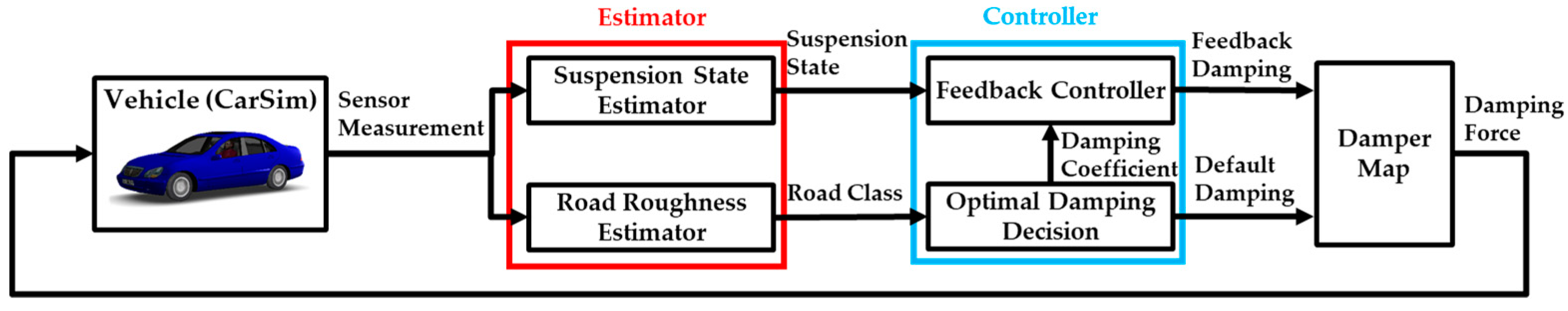
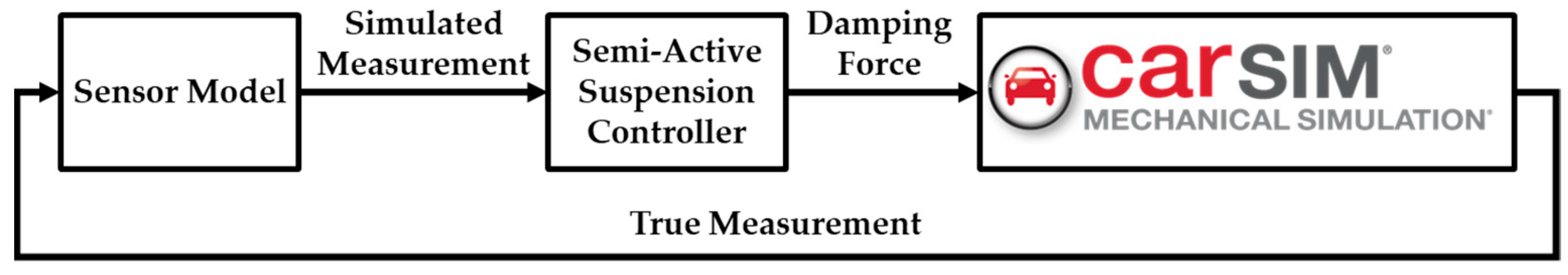
The proposed controller for the semi-active suspension system was designed to improve ride comfort under complex road disturbances with both low- and high-frequency components. Additionally, the controller was designed to utilize signals that are estimable, ensuring practical implementation in vehicles. To achieve these goals, the architecture of the proposed controller was organized as shown in Figure 1. The controller consists of two main modules: the estimator and the controller.
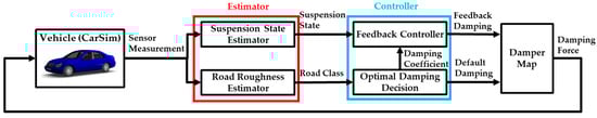
Figure 1.
Overall architecture of the proposed semi-active suspension system, which is composed of the estimator and controller. CarSim with a variable damper map was used as a plant model for the simulation study.
The estimator was designed with consideration for the vehicle’s available sensor configuration. In this study, an IMU on the vehicle body and two-wheel accelerometers on the front axle were used to estimate the dynamic states of the sprung and un-sprung masses. Along with the IMU and accelerometers, the estimator also utilized speed measurements from the wheel speed sensors, which are part of the anti-lock brake system. To process these sensor measurements and provide necessary information for the controller, the estimator included two sub-modules: the suspension state estimator and the road roughness estimator. The suspension state estimator calculates the roll rate, pitch rate, body velocity, and stroke rate, which are used by the feedback controller. The road roughness estimator uses acceleration measurements from the wheel accelerometer to classify road conditions into discrete categories based on ISO 8608 [62].
The controller module was composed of two sub-modules. First, the optimal damping decision module determines the linear damping coefficient according to the road class, aiming to minimize vertical acceleration and jerk caused by road surface roughness. The feedback controller then determines the additional suspension force needed to enhance ride comfort when the vehicle encounters low-frequency disturbances. The feedback gain of the controller was optimized using the LQSOF method, incorporating the damping coefficient provided by the optimal damping decision module. Finally, the outputs of the feedback controller and the optimal damping decision were combined to determine the damping force using the damping force–stroke rate curve of the semi-active damper.
3. Estimator Design
3.1. Suspension State Estimator
Conventional feedback controllers for suspension systems have been developed using various vehicle models, such as quarter-car, half-car, or full-car models. Regardless of the vehicle model, the vertical position of the sprung and un-sprung masses was used as a state variable. However, accurately measuring or estimating the vertical position of a vehicle using affordable sensors is quite challenging. Therefore, it is crucial to estimate as many vehicle states as possible within a limited sensor configuration to ensure the implementation of the feedback control in semi-active suspension systems.
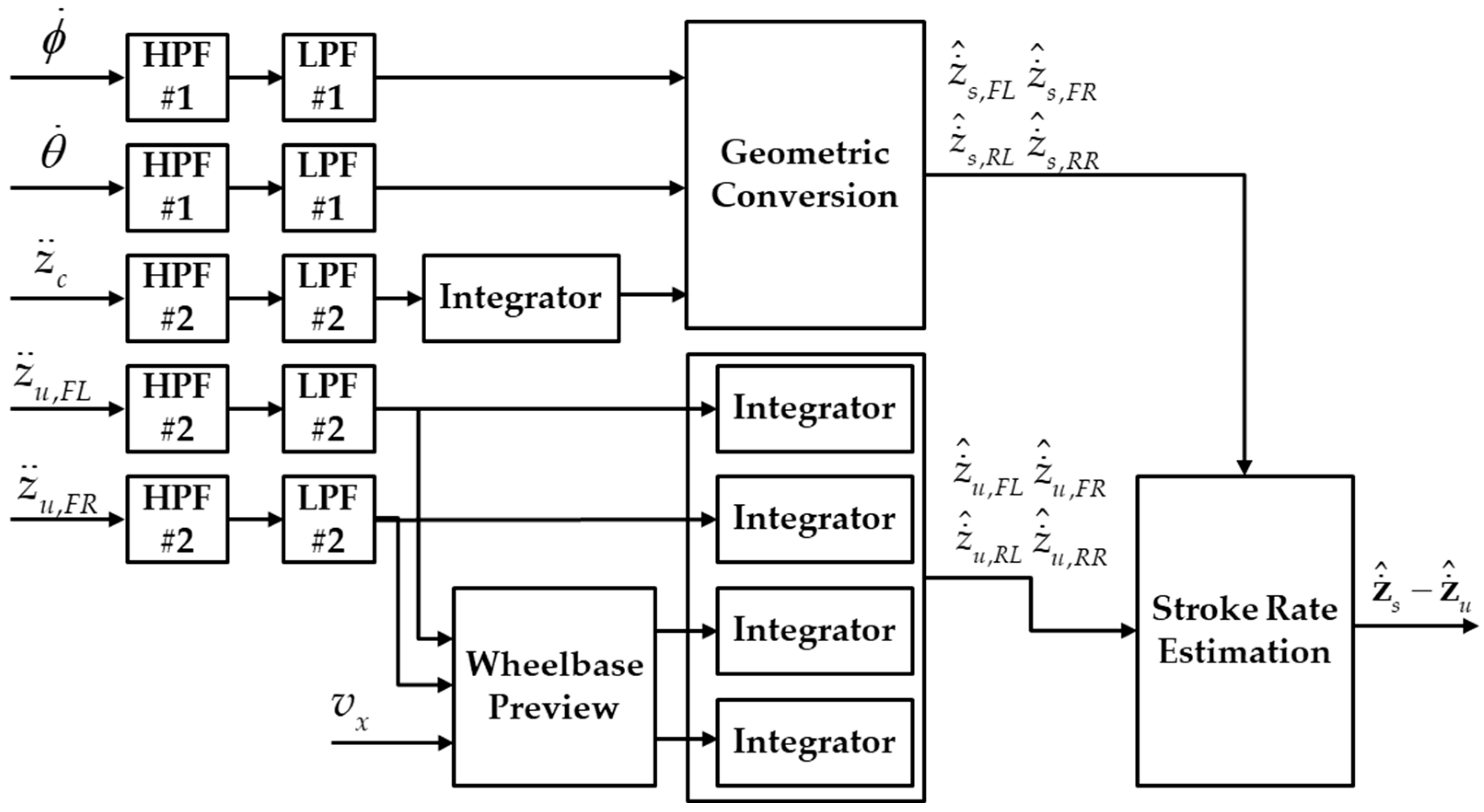
In this study, only three additional sensors—an IMU and two wheel accelerometers—were required to estimate the vehicle states needed for the controller of the semi-active suspension system. Given that the wheelbase of a passenger car is short enough to assume that the front and rear wheels encounter the same road conditions, a wheelbase preview concept was applied to virtually generate the acceleration measurements for the rear axle. Based on this sensor configuration and the wheelbase preview, the structure of the suspension state estimator is depicted in Figure 2.

Figure 2.
Block diagram of the suspension state estimator using high-pass filter (HPF) and low-pass filter (LPF) with vehicle geometry.
Measurements from the IMU and accelerometers were filtered using bandwidth filters to reduce the computational burden, avoiding the complexity of stochastic filters, such as the Kalman filter [63]. A high-pass filter (HPF) was applied to eliminate drift caused by the road slope or bank angle, while a low-pass filter (LPF) was used to reduce high-frequency noise from the sensors. Since accelerometers and gyroscopes have different measurement characteristics, the cut-off frequencies and damping ratios of the filters were set differently for each sensor type. As shown in Figure 2, HPF #1 and LPF #1 were applied to the gyroscope, while HPF #2 and LPF #2 were used for the accelerometers. The specific cut-off frequencies and damping ratios for each filter are summarized in Table 1. Since the IMU measures the variables that change relatively slowly, the damping ratio of HPF #1 and LPF #1 was set to 0.7. Meanwhile, the measurements of the accelerometers included a fast change, so the damping ratio of HPF #2 and LPF #2 was set to 0.5. The cut-off frequency of the bandwidth filters was determined by the data-driven approaches.

Table 1.
Specification of the bandwidth filters for the suspension state estimator.
The vertical velocity of the vehicle body, , was estimated by integrating the filtered signal of . After integration, the vertical velocity of the sprung mass corner, , was estimated by using the geometry of the vehicle body under the assumption of a rigid body, as follows:
where, tf and tr are the track width of the front and rear axles, respectively, while lf and lr are the distance of the front and rear axles from the center of gravity.
The vertical velocity of the un-sprung mass must be calculated before estimating the stroke rate. As mentioned earlier, the wheelbase preview was applied to estimate the acceleration of the rear axles at the k-th time stamp from the measurements of the front axles, as follows:
where L and vx are the wheelbase and longitudinal velocity of the vehicle, vx is the average of the output of the wheel speed sensors, and dt is the sampling time of the controller. Then, the vertical acceleration of the un-sprung masses was integrated to estimate the velocity, . Finally, the stroke rate of each corner was calculated, as follows:
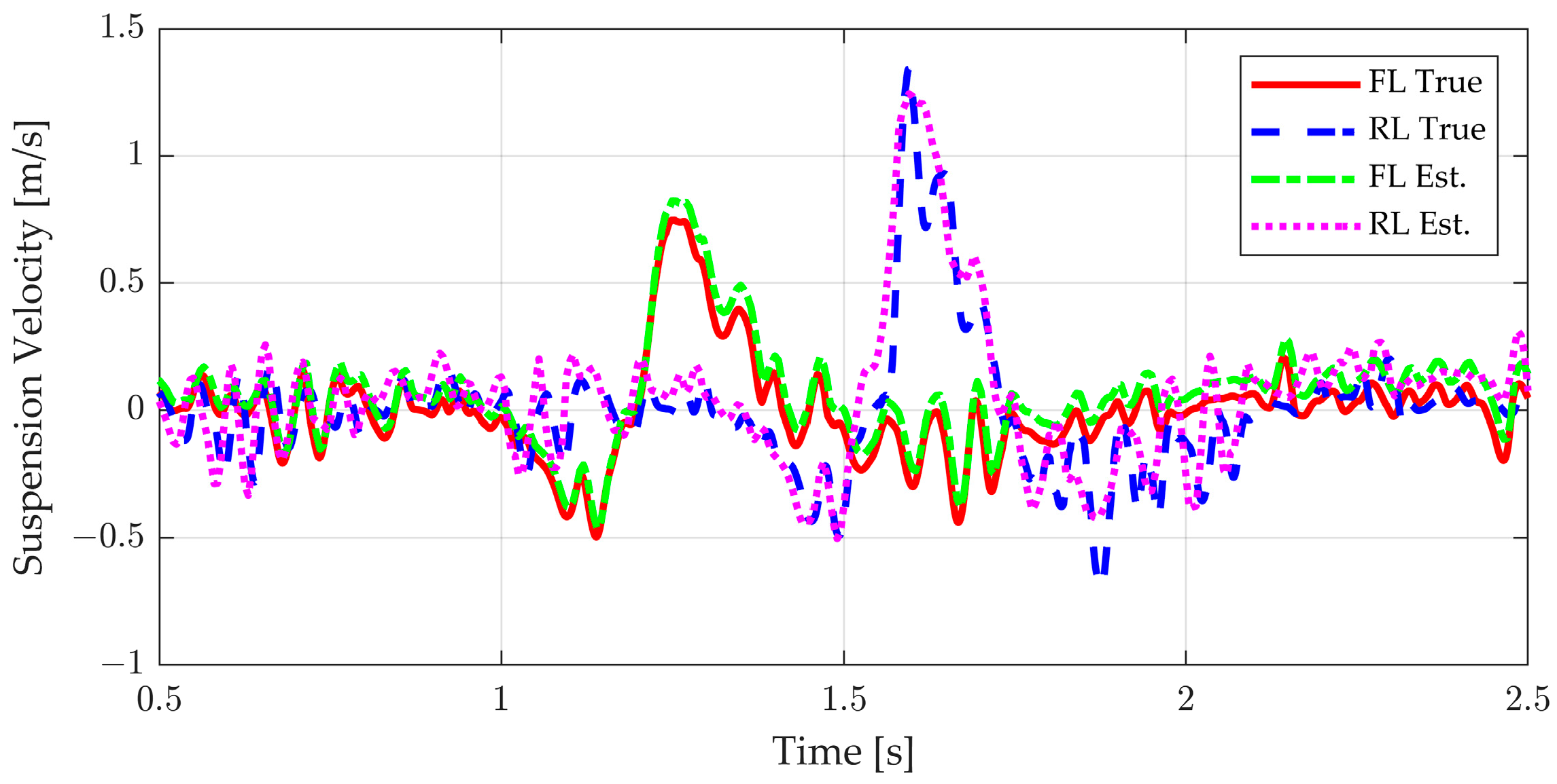
The evaluation results of the stroke rate estimation are provided in Figure 3. To verify the stroke rate estimation performance, a bump scenario with a roughness of a c class was used. As shown in Figure 3, the suspension state estimator showed an accurate stroke rate estimation performance in both the front and rear wheels without the occurrence of drift or bias, even in rough road conditions.
Figure 3.
Evaluation results of the stroke rate estimation.
3.2. Road Roughness Classifier
As previously mentioned, disturbances in the suspension system can be classified into two categories: low-frequency and high-frequency disturbances. Low-frequency disturbances, such as bumps or potholes, can be managed by the feedback controller. However, responding to high-frequency disturbances is challenging due to the response delay of the actuator. Therefore, the default damping curve of the variable damper should be adapted to minimize body vibration caused by high-frequency disturbances. The roughness of the road surface must be quantified in order to adjust the damping curve appropriately. Given that road roughness consists of disturbances across various frequencies, it is essential to classify road roughness into discrete categories.
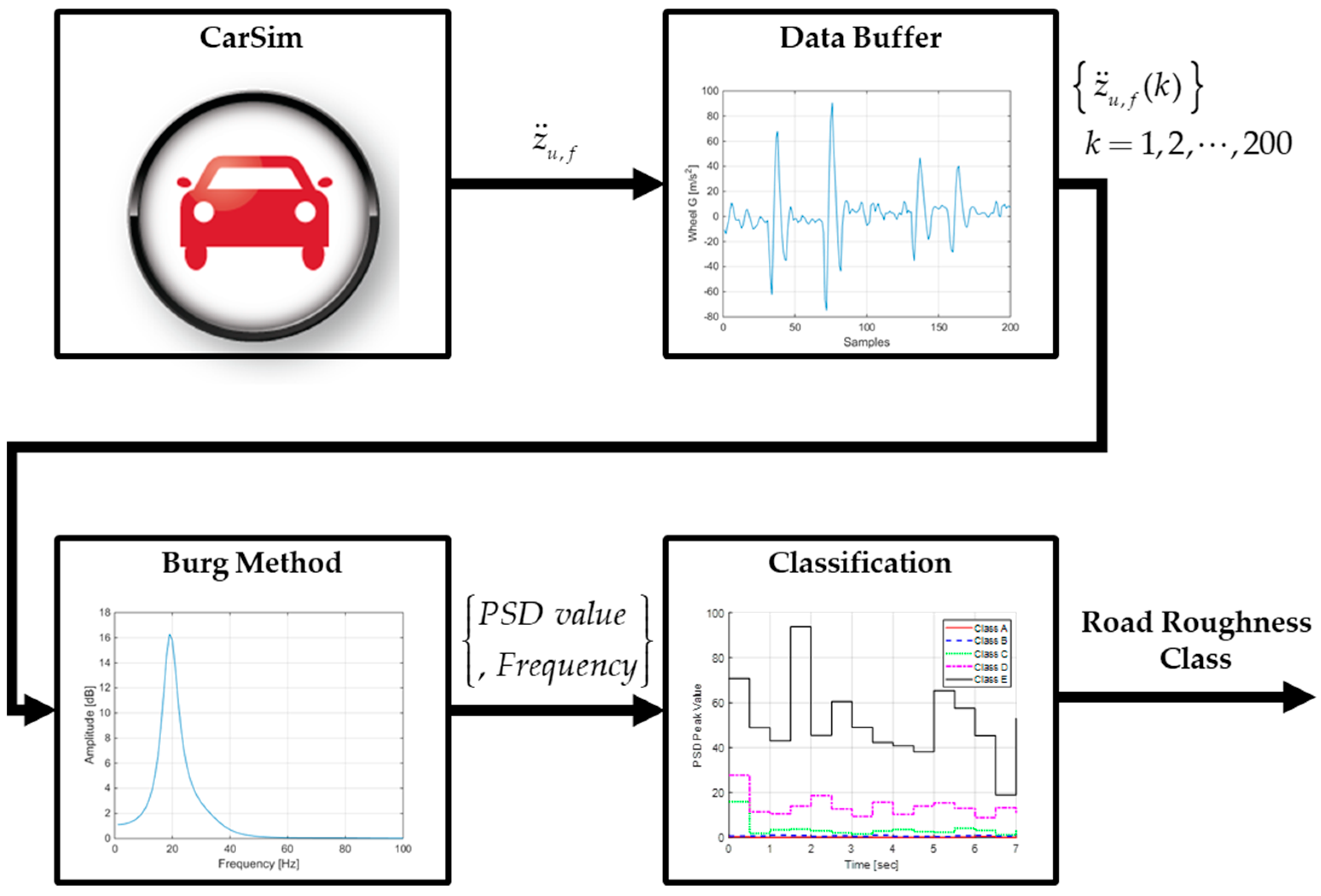
The accelerometer measurement from the front left wheel was used to classify road roughness according to the road surface profiles defined in ISO 8608. To analyze the signal in the frequency domain, the measurement must be accumulated. In this study, a moving window approach was employed to accumulate the acceleration measurements. The data buffer size was set to 200, and the first-in, first-out rule was applied to continuously update the road roughness class. The Burg method was then applied to the accumulated wheel acceleration data to identify the peak amplitude and frequency [64]. The Burg method estimates the PSD of the input data by applying an autoregressive (AR) model to the signal and minimizing both forward and backward prediction errors. At this stage, a recursive algorithm was employed to calculate the coefficients of the AR model. Unlike approaches such as the Yule–Walker equations, the Burg method performs effectively with short datasets and provides high-resolution spectral estimates for signals with closely spaced frequency components. For the simulation implementation of the Burg method, the Burg method block of MATLAB R2022b’s DSP System Toolbox was used. The overall procedure of the road roughness estimator is depicted in Figure 4.
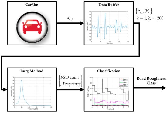
Figure 4.
Data flow of the road roughness classifier based on the Burg method for real-time spectral analysis of the wheel acceleration.
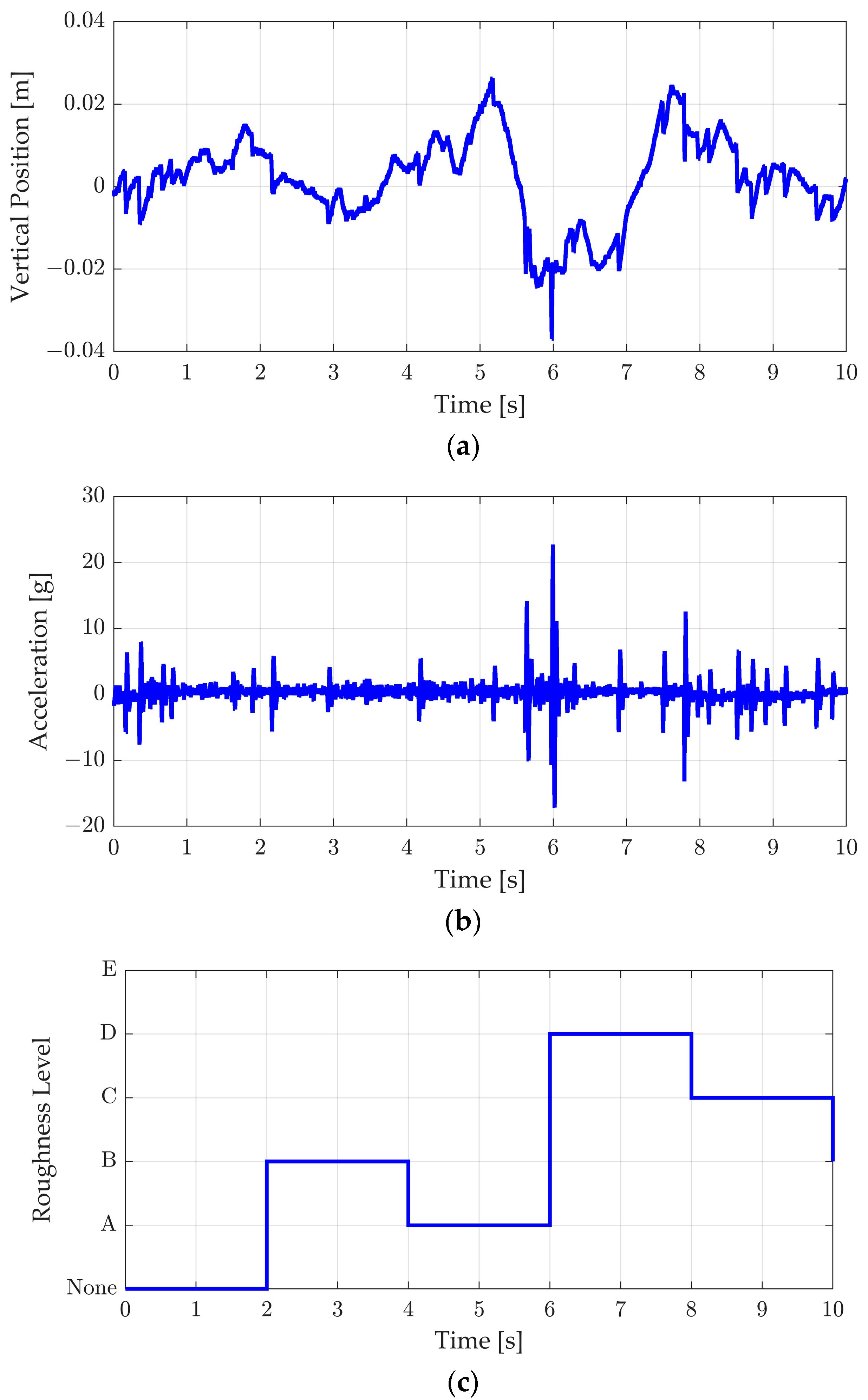
The results of the Burg method are illustrated in Figure 5. As shown in Figure 5a, which displays the vertical position of the front left wheel, the vehicle traversed surfaces with varying roughness. These changes in vertical position generated vertical wheel accelerations with different peak values, as shown in Figure 5b. The proposed road roughness estimator classified the vertical acceleration into levels A to E according to ISO 8608 standards. Given that the data buffer size was 200 and the estimator’s sampling time was 10 ms, the road roughness level was updated every two seconds. As demonstrated in Figure 5c, the road roughness level was accurately estimated in response to changes in vertical acceleration.
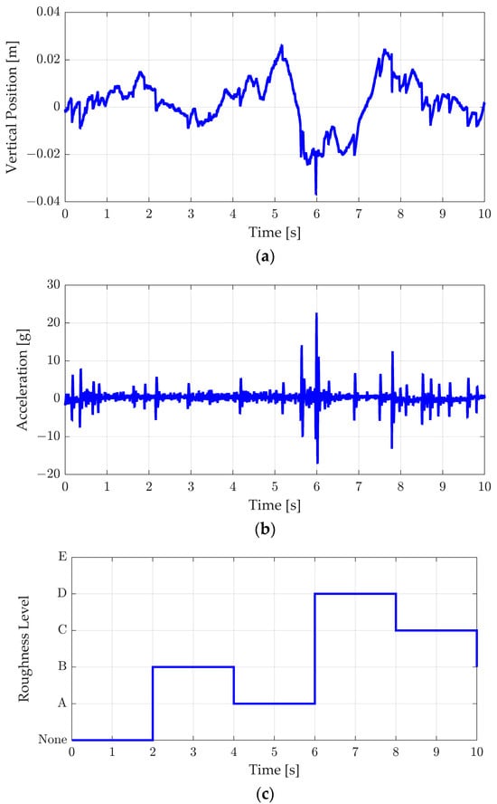
Figure 5.
Results of road roughness classification on the condition of the continuous changes in road roughness: (a) vertical position of the wheel center, (b) vertical acceleration of the wheel center, and (c) estimated road roughness level.
4. Controller Design
4.1. Feedback Controller
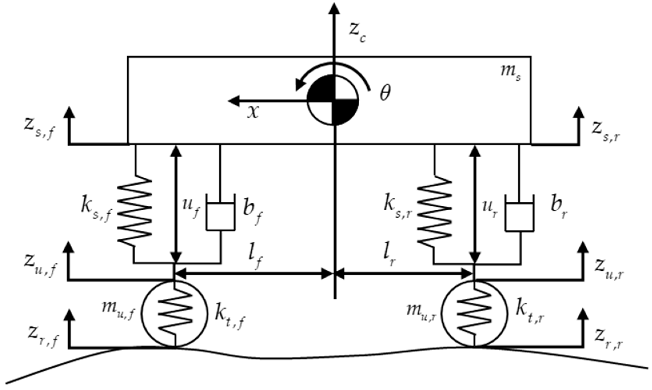
The objective of the proposed feedback controller was to enhance ride comfort by mitigating low-frequency disturbances. Specifically, the motion of the sprung mass should be minimized to reduce vertical acceleration and the pitch rate. Therefore, the vehicle model used for the feedback controller must include heave and pitch motions as state variables. In this study, a feedback controller for a semi-active suspension system was designed based on a half-car model, with consideration given to extending the design to a full-car model in future work. As illustrated in Figure 6, the half-car model was used to represent the heave and pitch motions of the sprung mass, along with the vertical motion of the un-sprung mass [65].
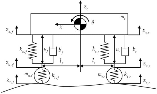
Figure 6.
Half-car model for controller design.
Before deriving the equations of motion, it is important to define the state and input variables. As shown in Figure 6, the heave and pitch angle of the sprung mass with respect to the fixed coordinate system are denoted as zc and θ, respectively. The vertical positions of the front and rear axles of the sprung mass are represented as zs,f and zs,r. The vertical positions of the un-sprung masses are denoted as zu,f and zu,r. The tire contact points with the road are defined as zr,f and zr,r. The inputs of the front and rear suspension systems are denoted as uf and ur.
Based on the state and input variables shown in Figure 6, the equations of motion for heave and pitch motions were derived, as given in (1):
where ms and Iy are the mass and pitch moment of inertia of the sprung mass, while lf and lr are the distance of the front and rear axle from the sprung mass’s center of gravity. In Equation (4), ff and fr are the force from the suspension system, which is calculated as follows under the assumption of the linear spring and damping:
where ks,f and ks,r are the spring stiffness of the front and rear suspension, bf and br are the damping coefficients of the front and rear suspension, while uf and ur are the control inputs of the front and rear suspension. Then, the equations of motion for the vertical motion of the un-sprung mass were derived, as follows:
where mu,f and mu,r are the mass of the un-sprung mass, while kt,f and kt,r the tire stiffness of the front and rear tires. From Equations (4)–(6), the equation of motion can be represented in a matrix-vector form, as follows:
The motion of the sprung mass is coupled with heave and pitch motion. Under the assumption of the rigid-body and small-angle approximation, zs,f and zs,r can be represented as a function of zc and θ, as follows:
Equation (8) can be represented in matrix-vector form, as follows:
By substituting Equation (9) into (7), the equation of motion for the half-car model was derived, as follows:
By augmenting the equation for sprung and un-sprung mass, the equation of motion for the half-car model was derived as follows, with the matrix M, K, B, U, and L and vectors z, u, and w:
The state equation of the half-car model was defined, as follows:
where x and u are the state and input vectors of the state equation, and I is an identity matrix, with dimensions in subscripts. As shown in (12), the state vector of the half-car model includes the vertical positions of the sprung and un-sprung masses as well as the pitch angle. However, accurately estimating these positions and orientations is challenging because the semi-active suspension system relies on accelerometers and an IMU. Therefore, it is essential to design an optimal feedback controller based on the available outputs. As mentioned in Section 3.1, the estimator, which uses the IMU and two-wheel accelerometers, can measure the roll rate and pitch rate, and estimate the body velocity and stroke rate. Since the proposed controller is based on the half-car model, the output equation was defined without the roll rate, as follows:
The control input of the static output feedback controller given as u in (12) was derived, as follows:
The optimal gain, KSOF, was obtained by solving the optimization problem in (15). The heuristic optimization method, covariance matrix adaptation-evolutionary strategy (CMA-ES), was applied to find the optimal KSOF:
where Q, N, and R are the weighting matrices for the LQSOF optimization, and P is the unknown symmetric matrix of the algebraic Riccati equation in (15).
4.2. Optimal Damping Controller
To respond effectively to high-frequency disturbances, the default damping curve of the semi-active damper should be adapted to minimize vertical vibrations of the sprung mass. Additionally, in the optimization problem presented in Section 4.1, linear damping was assumed to derive the linear state-space equation for the half-car model. However, because the actual damping characteristics of the damper were nonlinear, the performance of the LQR or LQSOF controller was limited, as the error in the linear damping assumption increased. In other words, the performance of the LQSOF controller was maximized when the damper behaved as a linear damper.
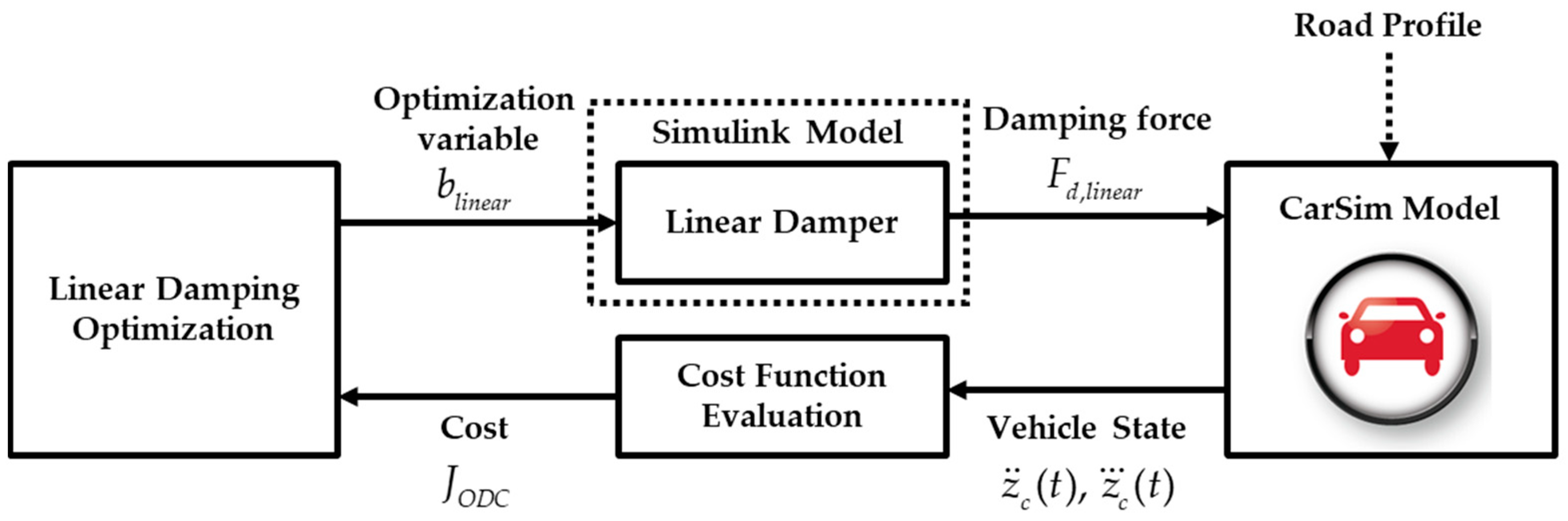
The optimal linear damping coefficient was defined for each road class according to ISO standards. Due to the nonlinearity of both the suspension and vehicle models, it was challenging to analytically determine the optimal damping coefficient. Therefore, this study introduced a numerical optimization method to determine the linear damping coefficient that minimizes vertical acceleration and jerk. The optimization procedure is summarized in Figure 7. To account for the nonlinearity of the vehicle model, the CarSim model—excluding the damper—was used as the plant model for optimization. The built-in damper of the CarSim model was replaced by a linear damper model in Simulink, which utilized the damping coefficient provided by the optimizer.
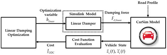
Figure 7.
Process of the linear damping coefficient optimization for ride comfort.
For optimization, the built-in MATLAB function, fminsearch(), was used to minimize the cost function, JODC. The Nelder–Mead simplex direct search algorithm was employed by fminsearch() to perform the optimization. The cost function, JODC, defined in (16), aims to minimize both acceleration and jerk. α was used in (16) to adjust the weight between acceleration and jerk. In this study, 0.1 was used for α. The optimization was conducted for class A, B, and C roads:
4.3. Damper Control Strategy
The feedback controller determines the additional suspension force needed to reduce vertical acceleration and pitch motion, while the optimal damping controller adjusts the linear damping coefficient to regulate vibrations caused by high-frequency noise. The damping coefficient, determined through offline optimization, was used to define B in Section 4.1. In other words, the optimal feedback gain was derived based on the optimal linear damping coefficient. As a result, the proposed controller can deliver improved performance under driving conditions where both high-frequency and low-frequency disturbances coexist.
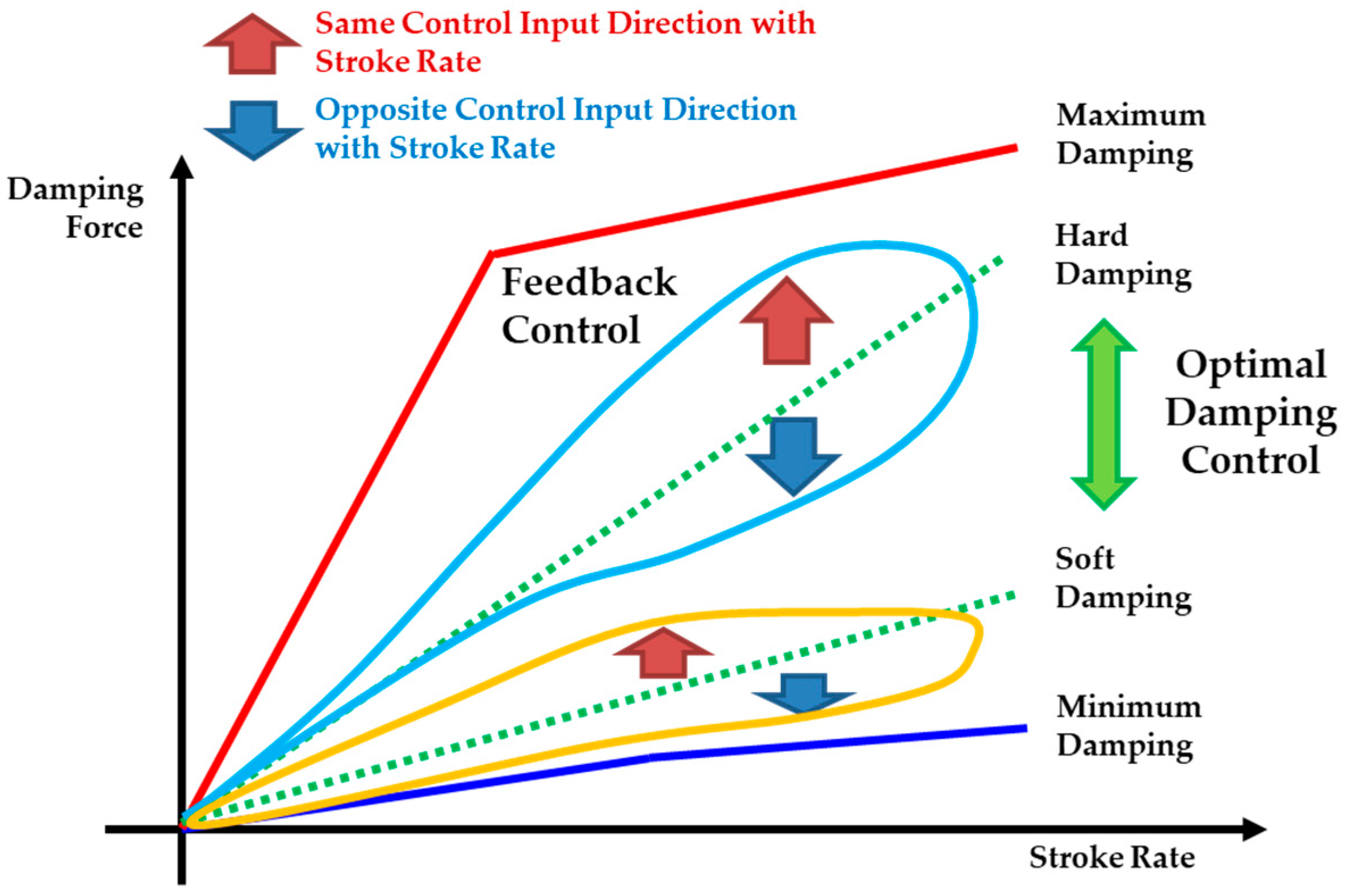
The control input for the semi-active damper was determined as illustrated in Figure 8. First, the linear damping coefficient was adjusted according to the estimated road class. Then, the damping force was actively modified to meet the control input from the feedback controller. If the control input was in the same direction as the stroke rate, the damping of the variable damper increased to generate the additional damping force required by the feedback control. Conversely, when the control input opposed the stroke rate, the damper was softened to comply with the feedback control’s input. Consequently, although the semi-active suspension system is based on a variable damper, the proposed control concept allowed it to achieve effects similar to those of an active suspension system.
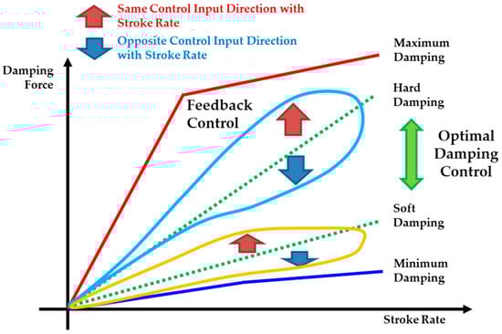
Figure 8.
Conceptual diagram of the damper control strategy based on optimal damping control, shown by the green dotted line, and feedback control, shown as red and blue arrows, from linear damping.
5. Simulation Results
The proposed road-adaptive SOF controller for the semi-active suspension system was evaluated through a simulation study. The configuration of the simulation setup is shown in Figure 9. A simulation environment was constructed using a co-simulation of MATLAB/Simulink and CarSim 2017.1. The proposed algorithm is represented as a single block named “semi-active suspension controller”. The vehicle model used was an E-Class Sedan, available as a bundled model in CarSim. The parameters of the vehicle model are summarized in Table 2. Among the parameters of the vehicle model in CarSim, only the parameters related to the half-car model were used for controller design and summarized in Table 2.

Figure 9.
Configuration of the simulation study with the sensor model and CarSim vehicle model.
Table 2.
Parameters for the vehicle model of the E-Class Sedan in CarSim.
Since CarSim provides true measurements of both observable and unobservable states, a sensor model was introduced to produce outputs that closely resemble those of actual IMUs and acceleration sensors. To enhance the agreement between simulation results and real-world vehicle testing, CarSim’s motion sensor function was employed to position the IMU on the sprung mass and acceleration sensors on the left and right lower arms of the front wheels.
For measurements from the IMU, accelerometer, and wheel speed sensors, a sensor model was implemented to mimic the characteristics of real sensors by incorporating sensor delay, amplitude adjustment, and discretization. Additionally, the sampling time of the controller and the system delay of the semi-active damper were aligned with those typically found in vehicle semi-active suspension systems. In this study, the actuator delay was modeled using a first-order time delay model. The parameters for the sensor, controller, and actuator models are summarized in Table 3. Furthermore, the tire–road friction coefficient was set at 0.85, assuming dry asphalt conditions. In addition, the feedback gains for the simulation study are summarized in Table 4.
Table 3.
Parameters for the sensor model, controller, and damper model.
Table 4.
Feedback controller gains.
Among the various vehicle states, vertical acceleration, pitch angle, and pitch rate were used to evaluate the proposed controller. Peak-to-peak (P2P), maximum, and minimum values were selected as key performance indicators (KPIs) for analyzing the simulation results. A total of nine KPIs, along with the time history of vehicle states, were compared between the proposed algorithm and a base algorithm. To assess performance, three comparison cases were established: The first case was a passive setup using the default nonlinear passive damper provided in CarSim. The second case employed only the feedback controller described in Section 4.1 to determine the damping force of the variable damper, with the default damping curve set to the nonlinear curve of the passive damper. This case is named Base #1. The third case was based on a skyhook controller that adapted the damping curve according to road conditions. This case is named Base #2.
A total of four simulation scenarios were designed based on a bump scenario. The bump used in the simulation was 3.6 m long and 10 cm high, in accordance with Korean road construction regulations. The vehicle traveled at 30 kph, using CarSim’s built-in speed controller. The path was set to ensure the vehicle traveled straight over the bump, minimizing roll and lateral motion. Four road roughness profiles were applied to the bump, ranging from an ideal surface with no roughness to profiles corresponding to class A, B, and C roughness levels.
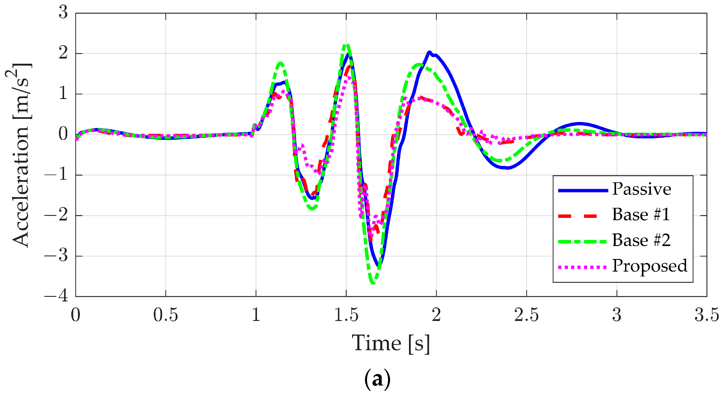
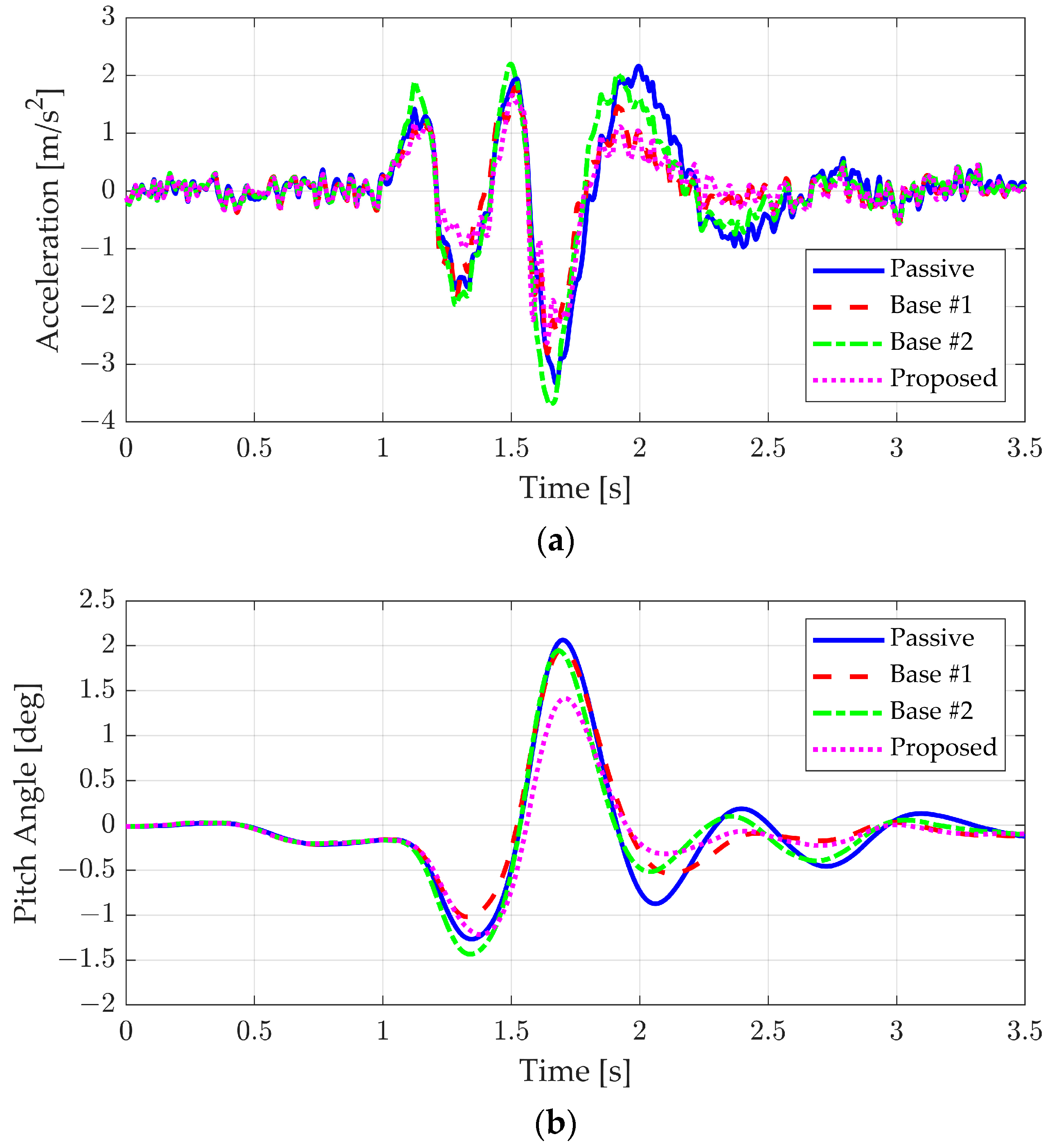
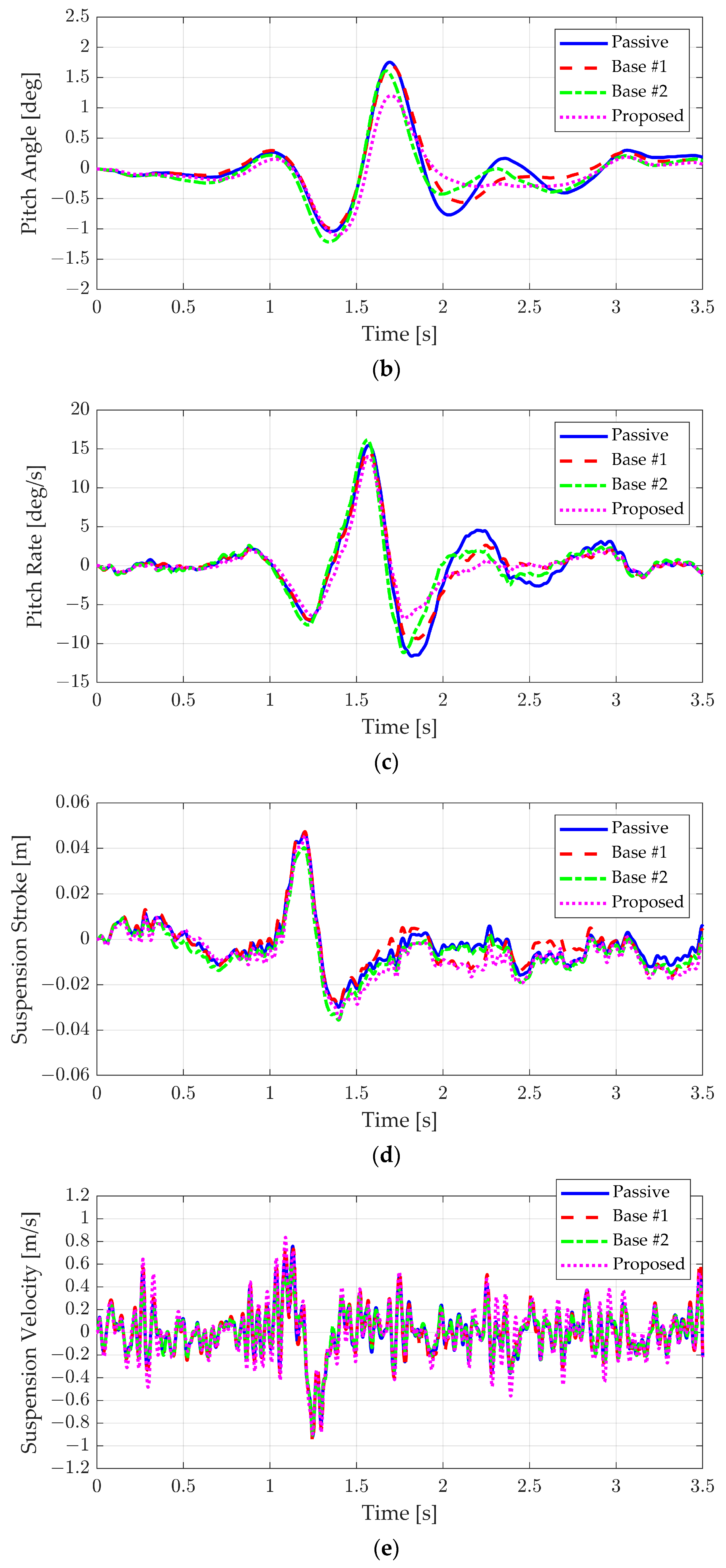
The simulation results for the ideal bump scenario are presented in Figure 10 and Table 5. The vertical acceleration history is shown in Figure 10a. The passive case and Base #2 exhibited higher vertical accelerations compared to the feedback controller. The limited performance improvement of Base #2, despite its damping control, is attributed to the difficulty in responding to low-frequency disturbances solely by adjusting the damping curve based on road roughness. Additionally, the discrete-time estimation of road roughness, necessary for real-time implementation in an embedded environment, prevents precise damping force control at every point on the bump. Conversely, both Base #1 and the proposed controller reduced the peak vertical acceleration. Since the road roughness profile was not applied in the ideal bump scenario, the performance of Base #1 and the proposed controller was nearly identical.
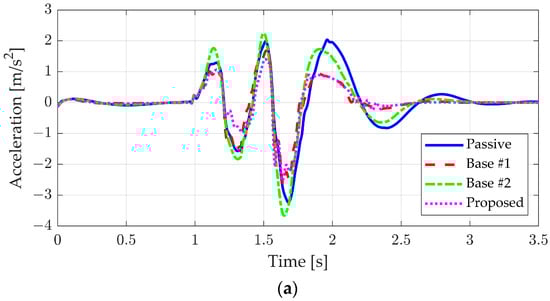
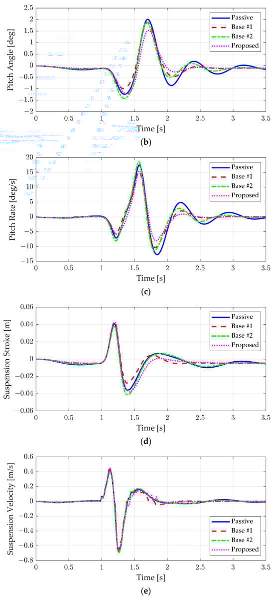
Figure 10.
Simulation results of the ideal case without road roughness: (a) vertical acceleration, (b) pitch angle, (c) pitch rate, (d) suspension stroke, and (e) suspension velocity.
Table 5.
KPIs of simulation results of the ideal case without road roughness.
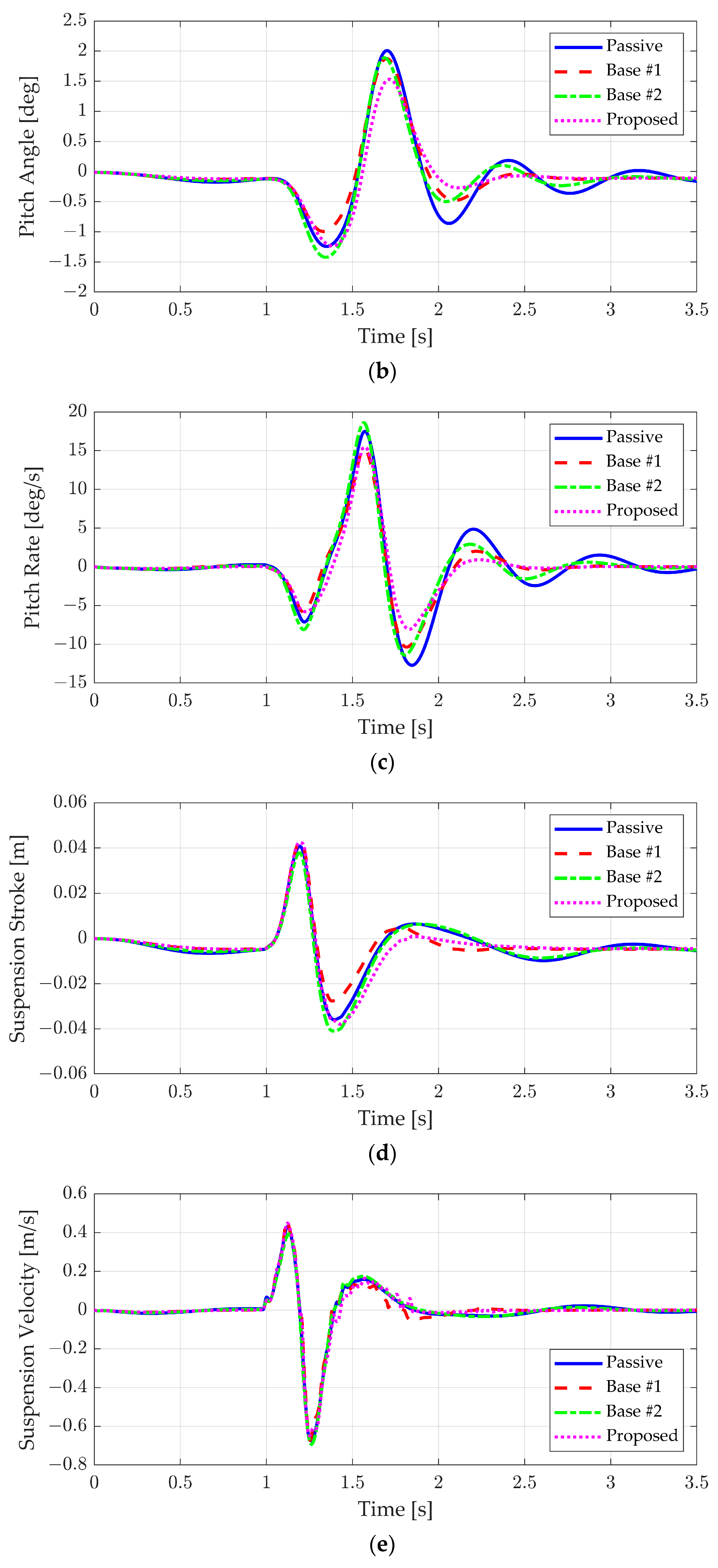
However, different behavior was observed in pitch motion, as depicted in Figure 10b,c. Since Base #2 requires the Burg method’s window duration to update the road class, it reduces pitch motion after the front wheels pass the bump. As a result, the pitch motion is reduced after 2 s with Base #2. Similar to the vertical acceleration, both Base #1 and the proposed controller effectively regulated the pitch angle and pitch rate. Notably, the proposed controller provided better pitch regulation than Base #1, as it adjusted the default damping to behave linearly, satisfying the assumptions of the feedback controller. The KPIs for the ideal bump scenario are summarized in Table 5, where the proposed algorithm demonstrated improvements over the base algorithm in maximum, minimum, and peak-to-peak values for vertical acceleration, pitch angle, and pitch rate. In particular, it can be seen that the improvement in the vertical acceleration was remarkable.
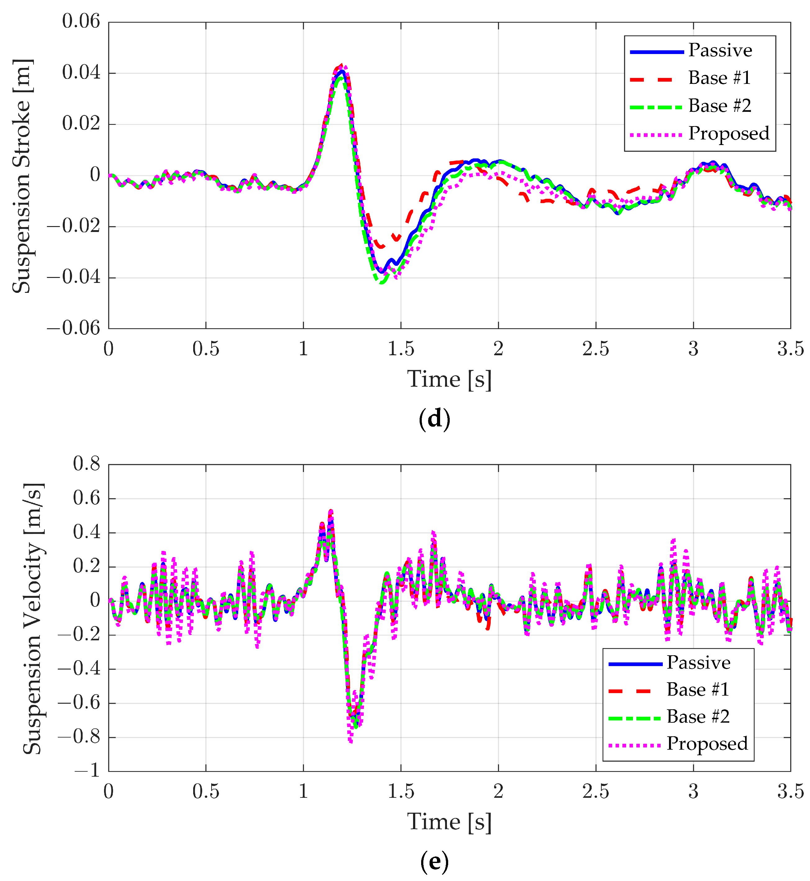
The simulation results for the bump with class A roughness are summarized in Figure 11 and Table 6. When class A roughness was applied, the overall trend mirrored that observed on the ideal road surface. However, the difference between Base #1 and the proposed algorithm became more pronounced due to the adaptation of the default damping. Specifically, the peak values of the proposed algorithm, shown in Figure 11a–c, were further reduced compared to those of Base #1. Additionally, the stroke was more effectively suppressed after the vehicle passed over the bump, as compared to the base algorithms. This overall improvement in performance was further evidenced by the larger differences in KPIs from the base algorithm, as presented in Table 6. Compared to the ideal bump case, where the improvement in the vertical acceleration was large, in the road roughness class A, a clear improvement could be seen not only for vertical acceleration but also for pitch motion.
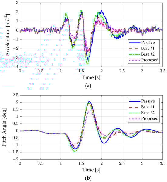
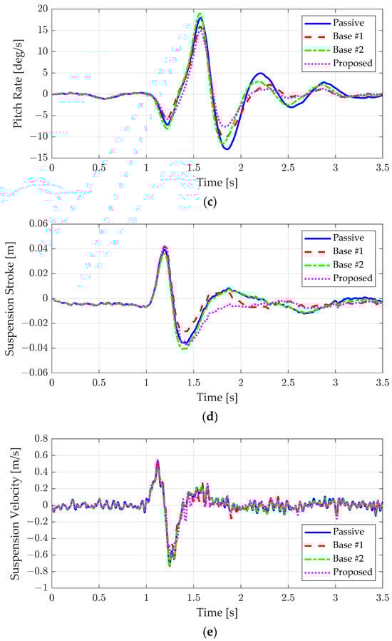
Figure 11.
Simulation results of road roughness class A: (a) vertical acceleration, (b) pitch angle, (c) pitch rate, (d) suspension stroke, and (e) suspension velocity.
Table 6.
KPIs of simulation results of road roughness class A.
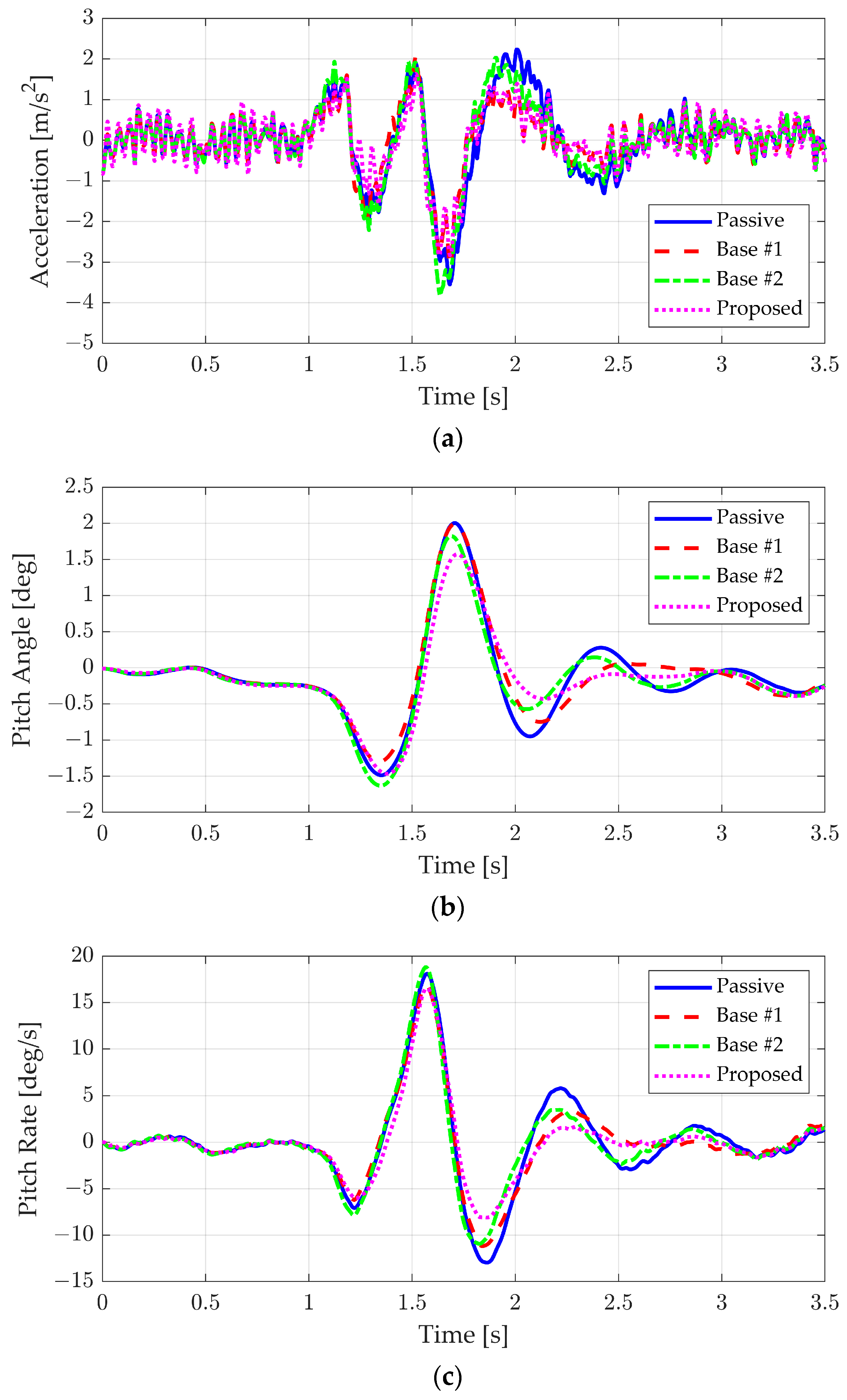
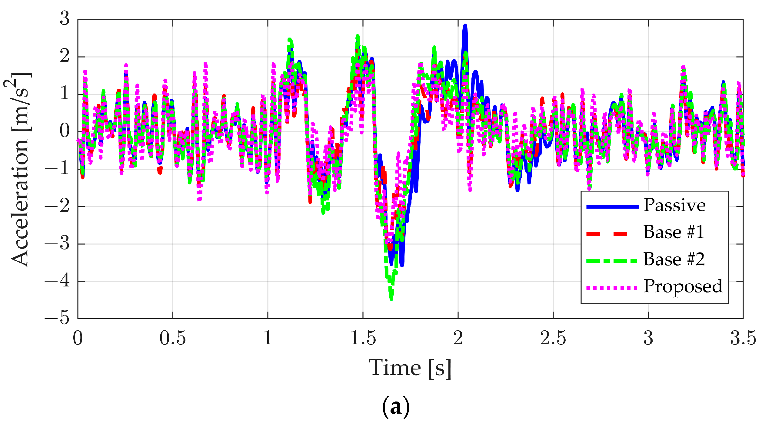
Figure 12 and Figure 13, along with Table 7 and Table 8, summarize the results for the bump scenario when classes B and C, representing rougher road conditions, were applied. The performance of Base #1, which used only the feedback controller, deteriorated as road roughness increased due to high-frequency disturbances. In contrast, Base #2, which adjusted the default damping according to road roughness, showed a slight improvement in vertical acceleration and pitch behavior. However, because Base #2 struggled to effectively respond to low-frequency disturbances, it did not achieve the same level of performance as Base #1. On the other hand, the proposed algorithm, which addressed both road surface roughness and bump response, maintained ride comfort even under rough road conditions. As shown in Table 7 and Table 8, it can be seen that an improvement in vertical acceleration and pitch motion similar to the results in the ideal bump case appeared even when the road surface was rough.


Figure 12.
Simulation results of road roughness class B: (a) vertical acceleration, (b) pitch angle, (c) pitch rate, (d) suspension stroke, and (e) suspension velocity.
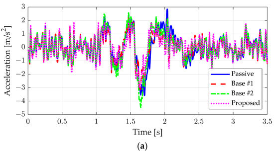
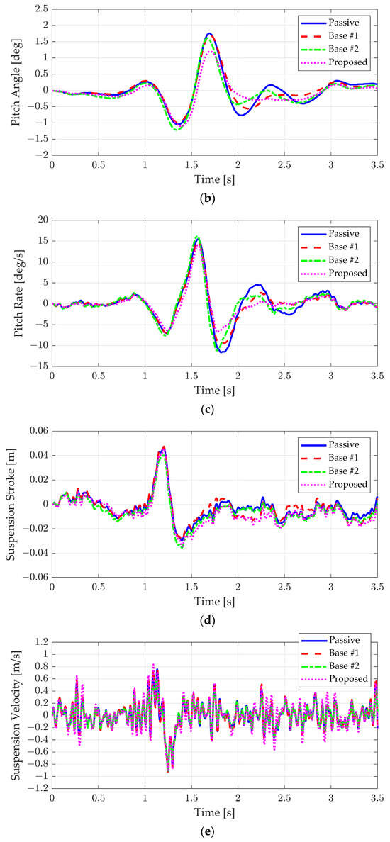
Figure 13.
Simulation results of road roughness class C: (a) vertical acceleration, (b) pitch angle, (c) pitch rate, (d) suspension stroke, and (e) suspension velocity.
Table 7.
KPIs of simulation results of road roughness class B.
Table 8.
KPIs of simulation results of road roughness class C.
6. Conclusions
A control algorithm for semi-active suspension was proposed to enhance ride comfort in scenarios where low-frequency and high-frequency disturbances occurred simultaneously. To achieve this, the proposed controller consisted of two sub-controllers: an optimal damping controller and a static output feedback controller. The necessary information for the controller was estimated by the vehicle state estimator and road roughness classifier, utilizing only the commercial sensors of the semi-active suspension system. Based on the road roughness, the default linear damping of the variable damper was adjusted to minimize vertical acceleration and jerk under high-frequency disturbances. Subsequently, the optimal feedback gain of the static output feedback controller was derived concerning the damping coefficient from the optimal damping controller, enabling an effective response to low-frequency disturbances, such as bumps and potholes. The proposed algorithm was evaluated through simulation studies based on co-simulation between CarSim and MATLAB/Simulink. The results demonstrated that the algorithm improved ride comfort across bump scenarios under various road roughness conditions.
The proposed algorithm can be enhanced in three key areas. Firstly, it currently relies solely on an IMU and accelerometers, which measure road disturbances after they occur. Incorporating sensors such as cameras and LiDAR could provide disturbance profiles in advance. Integrating this preview information with feedback control could further improve performance against low-frequency disturbances. Secondly, the effectiveness of suspension control could be enhanced by integrating it with other chassis control systems beyond the variable damper. With the rise of vehicle electrification, motors are increasingly being installed on the front and rear wheels. Even when control force cannot be applied using the semi-active damper, pitch moments could be generated without additional actuators by leveraging the driving motors, thereby improving ride comfort through cooperative control between the variable damper and the drive motor. Finally, introducing a learning-based controller could significantly improve control performance. Semi-active suspension systems exhibit significant nonlinearity and can apply control only in specific directions. The nonlinearity of variable dampers, in particular, is challenging to model, complicating controller design. In this context, implementing a controller through reinforcement learning could be an effective approach.
Author Contributions
Conceptualization, D.K. and Y.J.; methodology, Y.J.; software, D.K. and Y.J.; validation, D.K. and Y.J.; formal analysis, Y.J.; investigation, Y.J.; resources, Y.J.; data curation, Y.J.; writing—original draft preparation, Y.J.; writing—review and editing, Y.J.; visualization, D.K. and Y.J.; supervision, Y.J.; project administration, Y.J.; funding acquisition, Y.J. All authors have read and agreed to the published version of the manuscript.
Funding
This research was supported by the Basic Science Research Program through the National Research Foundation of Korea (NRF), funded by the Ministry of Education (NRF-2019R1A6A1A03032119).
Institutional Review Board Statement
Not applicable.
Informed Consent Statement
Not applicable.
Data Availability Statement
Data are contained within the article.
Conflicts of Interest
The authors declare no conflicts of interest.
Nomenclatures
| Symbol | Meaning |
| Roll rate of the sprung mass | |
| Pitch rate of the sprung mass | |
| zc | Vertical position of the sprung mass |
| zs,FL, zs,FR, zs,RL, zs,RR | Vertical position of the front left, front right, rear left, and rear right corner of the sprung mass |
| zs,f, zs,r | Vertical position of the front and rear axle of the sprung mass |
| zu,FL, zu,FR, zu,RL, zu,RR | Vertical position of the front left, front right, rear left, and rear right un-sprung mass |
| zu,f, zu,r | Vertical position of the front and rear un-sprung mass |
| vx | Longitudinal velocity of the vehicle |
| tf, tr | Track width of the front and rear axles |
| lf, lr | Distance of the front and rear axles from the center of gravity of the sprung mass |
| L | Wheelbase of the vehicle |
| dt | Sampling time of the controller |
| ms | Mass of the sprung mass |
| mu,f, mu,r | Mass of the front and rear sprung mass |
| Iy | Pitch moment of inertia of the sprung mass |
| ks,f, ks,r | Spring stiffness of the front and rear suspension |
| bf, br | Damping coefficients of the front and rear suspension |
| kt,f, kt,r | Tire stiffness of the front and rear tires |
| zr,f, zr,r | Tire contact points with the road of the front and rear tires |
| uf, ur | Control inputs of the front and rear suspension |
| ff, fr | Front and rear suspension force |
References
- Sharp, R.; Crolla, D. Road vehicle suspension system design—A review. Veh. Syst. Dyn. 1987, 16, 167–192. [Google Scholar] [CrossRef]
- Jiregna, I.; Sirata, G. A review of the vehicle suspension system. J. Mech. Energy Eng. 2020, 4, 109–114. [Google Scholar] [CrossRef]
- Sharp, R.; Hassan, S. The relative performance capabilities of passive, active and semi-active car suspension systems. Proc. Inst. Mech. Eng. Part D Transp. Eng. 1986, 200, 219–228. [Google Scholar] [CrossRef]
- Soliman, A.; Kaldas, M. Semi-active suspension systems from research to mass-market—A review. J. Low Freq. Noise Vib. Act. Control 2021, 40, 1005–1023. [Google Scholar] [CrossRef]
- Olivier, M.; Sohn, J.W. Design and geometric parameter optimization of hybrid magnetorheological fluid damper. J. Mech. Sci. Technol. 2020, 34, 2953–2960. [Google Scholar] [CrossRef]
- Strecker, Z.; Roupec, J.; Mazůrek, I.; Macháček, O.; Kubík, M. Influence of response time of magnetorheological valve in Skyhook controlled three-parameter damping system. Adv. Mech. Eng. 2018, 10, 1687814018811193. [Google Scholar] [CrossRef]
- Ding, R.; Wang, R.; Meng, X.; Chen, L. A modified energy-saving skyhook for active suspension based on a hybrid electromagnetic actuator. J. Vib. Control 2019, 25, 286–297. [Google Scholar] [CrossRef]
- Knap, L.; Makowski, M.; Siczek, K.; Kubiak, P.; Mrowicki, A. Hydraulic vehicle damper controlled by piezoelectric valve. Sensors 2023, 23, 2007. [Google Scholar] [CrossRef] [PubMed]
- Li, F.; Yuan, S.; Qian, F.; Wu, Z.; Pu, H.; Wang, M.; Ding, J.; Sun, Y. Adaptive deterministic vibration control of a piezo-actuated active–passive isolation structure. Appl. Sci. 2021, 11, 3338. [Google Scholar] [CrossRef]
- Mikułowski, G.; Wiszowaty, R.; Holnicki-Szulc, J. Characterization of a piezoelectric valve for an adaptive pneumatic shock absorber. Smart Mater. Struct. 2013, 22, 125011. [Google Scholar] [CrossRef]
- Tseng, H.E.; Hrovat, D. State of the art survey: Active and semi-active suspension control. Veh. Syst. Dyn. 2015, 53, 1034–1062. [Google Scholar] [CrossRef]
- Desai, R.; Guha, A.; Seshu, P. A comparison of quarter, half and full car models for predicting vibration attenuation of an occupant in a vehicle. J. Vib. Eng. Technol. 2021, 9, 983–1001. [Google Scholar] [CrossRef]
- Youn, I.; Ahmad, E. Anti-jerk optimal preview control strategy to enhance performance of active and semi-active suspension systems. Electronics 2022, 11, 1657. [Google Scholar] [CrossRef]
- Karkoub, M.A.; Zribi, M. Active/semi-active suspension control using magnetorheological actuators. Int. J. Syst. Sci. 2006, 37, 35–44. [Google Scholar] [CrossRef]
- Unger, A.; Schimmack, F.; Lohmann, B.; Schwarz, R. Application of LQ-based semi-active suspension control in a vehicle. Control Eng. Pract. 2013, 21, 1841–1850. [Google Scholar] [CrossRef]
- Chen, M.Z.; Hu, Y.; Li, C.; Chen, G. Semi-active suspension with semi-active inerter and semi-active damper. IFAC Proc. Vol. 2014, 47, 11225–11230. [Google Scholar] [CrossRef]
- Wang, G.; Chen, C.; Yu, S. Optimization and static output-feedback control for half-car active suspensions with constrained information. J. Sound Vib. 2016, 378, 1–13. [Google Scholar] [CrossRef]
- Park, M.; Yim, S. Design of static output feedback and structured controllers for active suspension with quarter-car model. Energies 2021, 14, 8231. [Google Scholar] [CrossRef]
- Yao, J.-L.; Shi, W.-K.; Zheng, J.-Q.; Zhou, H.-P. Development of a sliding mode controller for semi-active vehicle suspensions. J. Vib. Control 2013, 19, 1152–1160. [Google Scholar] [CrossRef]
- Chen, B.-C.; Shiu, Y.-H.; Hsieh, F.-C. Sliding-mode control for semi-active suspension with actuator dynamics. Veh. Syst. Dyn. 2011, 49, 277–290. [Google Scholar] [CrossRef]
- Aljarbouh, A.; Fayaz, M.; Qureshi, M.S.; Boujoudar, Y. Hybrid sliding mode control of full-car semi-active suspension systems. Symmetry 2021, 13, 2442. [Google Scholar] [CrossRef]
- Nguyen, M.-Q.; Canale, M.; Sename, O.; Dugard, L. A Model Predictive Control approach for semi-active suspension control problem of a full car. In Proceedings of the 2016 IEEE 55th Conference on Decision and Control (CDC), Las Vegas, NV, USA, 12–14 December 2016; pp. 721–726. [Google Scholar]
- Poussot-Vassal, C.; Savaresi, S.M.; Spelta, C.; Sename, O.; Dugard, L. A methodology for optimal semi-active suspension systems performance evaluation. In Proceedings of the 49th IEEE Conference on Decision and Control (CDC), Atlanta, GA, USA, 15–17 December 2010; pp. 2892–2897. [Google Scholar]
- Canale, M.; Milanese, M.; Novara, C. Semi-active suspension control using “fast” model-predictive techniques. IEEE Trans. Control Syst. Technol. 2006, 14, 1034–1046. [Google Scholar] [CrossRef]
- Morato, M.M.; Nguyen, M.Q.; Sename, O.; Dugard, L. Design of a fast real-time LPV model predictive control system for semi-active suspension control of a full vehicle. J. Frankl. Instig. 2019, 356, 1196–1224. [Google Scholar] [CrossRef]
- Houzhong, Z.; Jiasheng, L.; Chaochun, Y.; Xiaoqiang, S.; Yingfeng, C. Application of explicit model predictive control to a vehicle semi-active suspension system. J. Low Freq. Noise Vib. Act. Control 2020, 39, 772–786. [Google Scholar] [CrossRef]
- Huang, D.-S.; Zhang, J.-Q.; Liu, Y.-L. The PID semi-active vibration control on nonlinear suspension system with time delay. Int. J. Intell. Transp. Syst. Res. 2018, 16, 125–137. [Google Scholar] [CrossRef]
- Ab Talib, M.H.; Mat Darus, I.Z.; Mohd Samin, P.; Mohd Yatim, H.; Ardani, M.I.; Shaharuddin, N.M.R.; Hadi, M.S. Vibration control of semi-active suspension system using PID controller with advanced firefly algorithm and particle swarm optimization. J. Ambient Intell. Humaniz. Comput. 2021, 12, 1119–1137. [Google Scholar] [CrossRef]
- Li, M.; Xu, J.; Wang, Z.; Liu, S. Optimization of the Semi-Active-Suspension Control of BP Neural Network PID Based on the Sparrow Search Algorithm. Sensors 2024, 24, 1757. [Google Scholar] [CrossRef] [PubMed]
- Emura, J.; Kakizaki, S.; Yamaoka, F.; Nakamura, M. Development of the semi-active suspension system based on the sky-hook damper theory. In SAE Transactions; Society of Automotive Engineering, Inc.: Warrendale, PA, USA, 1994; pp. 1110–1119. [Google Scholar]
- Liu, C.; Chen, L.; Yang, X.; Zhang, X.; Yang, Y. General theory of skyhook control and its application to semi-active suspension control strategy design. IEEE Access 2019, 7, 101552–101560. [Google Scholar] [CrossRef]
- Suzuki, T.; Mae, M.; Takeuchi, T.; Fujimoto, H.; Katsuyama, E. Model-based filter design for triple skyhook control of in-wheel motor vehicles for ride comfort. IEEJ J. Ind. Appl. 2021, 10, 310–316. [Google Scholar] [CrossRef]
- Lam, A.H.-F.; Liao, W.-H. Semi-active control of automotive suspension systems with magneto-rheological dampers. Int. J. Veh. Des. 2003, 33, 50–75. [Google Scholar] [CrossRef]
- Savaresi, S.M.; Spelta, C. A single-sensor control strategy for semi-active suspensions. IEEE Trans. Control Syst. Technol. 2008, 17, 143–152. [Google Scholar] [CrossRef]
- Yang, X.; Song, H.; Shen, Y.; Liu, Y.; He, T. Control of the vehicle inertial suspension based on the mixed skyhook and power-driven-damper strategy. IEEE Access 2020, 8, 217473–217482. [Google Scholar] [CrossRef]
- Qin, W.; Liu, F.; Yin, H.; Huang, J. Constraint-based adaptive robust control for active suspension systems under the sky-hook model. IEEE Trans. Ind. Electron. 2021, 69, 5152–5164. [Google Scholar] [CrossRef]
- Papaioannou, G.; Koulocheris, D.; Velenis, E. Skyhook control strategy for vehicle suspensions based on the distribution of the operational conditions. Proc. Inst. Mech. Eng. Part D J. Automob. Eng. 2021, 235, 2776–2790. [Google Scholar] [CrossRef]
- Liu, C.; Chen, L.; Lee, H.P.; Yang, Y.; Zhang, X. Generalized skyhook-groundhook hybrid strategy and control on vehicle suspension. IEEE Trans. Veh. Technol. 2022, 72, 1689–1700. [Google Scholar] [CrossRef]
- Díaz-Choque, C.S.; Félix-Herrán, L.; Ramírez-Mendoza, R.A. Optimal skyhook and Groundhook control for semiactive suspension: A comprehensive methodology. Shock Vib. 2021, 2021, 8084343. [Google Scholar] [CrossRef]
- Savaia, G.; Formentin, S.; Panzani, G.; Corno, M.; Savaresi, S.M. Enhancing skyhook for semi-active suspension control via machine learning. IFAC J. Syst. Control 2021, 17, 100161. [Google Scholar] [CrossRef]
- Lee, A.S.; Gadsden, S.A.; Al-Shabi, M. Application of nonlinear estimation strategies on a magnetorheological suspension system with skyhook control. In Proceedings of the 2020 IEEE International IOT, Electronics and Mechatronics Conference (IEMTRONICS), Vancouver, BC, Canada, 9–12 September 2020; pp. 1–6. [Google Scholar]
- Koch, G.; Kloiber, T.; Lohmann, B. Nonlinear and filter based estimation for vehicle suspension control. In Proceedings of the 49th IEEE Conference on Decision and Control (CDC), Atlanta, GA, USA, 15–17 December 2010; pp. 5592–5597. [Google Scholar]
- Pletschen, N.; Badur, P. Nonlinear state estimation in suspension control based on takagi-sugeno model. IFAC Proc. Vol. 2014, 47, 11231–11237. [Google Scholar] [CrossRef]
- Sisi, Z.A.; Mirzaei, M.; Rafatnia, S. Estimation of vehicle suspension dynamics with data fusion for correcting measurement errors. Measurement 2024, 231, 114438. [Google Scholar] [CrossRef]
- Jeong, K.; Choi, S.B. Vehicle suspension relative velocity estimation using a single 6-D IMU sensor. IEEE Trans. Veh. Technol. 2019, 68, 7309–7318. [Google Scholar] [CrossRef]
- Pham, T.P.; Sename, O.; Dugard, L. A nonlinear parameter varying observer for real-time damper force estimation of an automotive electro-rheological suspension system. Int. J. Robust Nonlinear Control 2021, 31, 8183–8205. [Google Scholar] [CrossRef]
- Pham, T.-P.; Sename, O.; Dugard, L. Real-time damper force estimation of vehicle electrorheological suspension: A nonlinear parameter varying approach. IFAC-Pap. 2019, 52, 94–99. [Google Scholar] [CrossRef]
- Weispfenning, T.; Leonhardt, S. Model-based identification of a vehicle suspension using parameter estimation and neural networks. IFAC Proc. Vol. 1996, 29, 4510–4515. [Google Scholar] [CrossRef]
- Pence, B.L.; Fathy, H.K.; Stein, J.L. Sprung mass estimation for off-road vehicles via base-excitation suspension dynamics and recursive least squares. In Proceedings of the 2009 American Control Conference, St. Louis, MO, USA, 10–12 June 2009; pp. 5043–5048. [Google Scholar]
- Thite, A.; Banvidi, S.; Ibicek, T.; Bennett, L. Suspension parameter estimation in the frequency domain using a matrix inversion approach. Veh. Syst. Dyn. 2011, 49, 1803–1822. [Google Scholar] [CrossRef]
- Na, J.; Huang, Y.; Wu, X.; Gao, G.; Herrmann, G.; Jiang, J.Z. Active adaptive estimation and control for vehicle suspensions with prescribed performance. IEEE Trans. Control Syst. Technol. 2017, 26, 2063–2077. [Google Scholar] [CrossRef]
- Zhang, Q.; Hou, J.; Hu, X.; Yuan, L.; Jankowski, Ł.; An, X.; Duan, Z. Vehicle parameter identification and road roughness estimation using vehicle responses measured in field tests. Measurement 2022, 199, 111348. [Google Scholar] [CrossRef]
- Zhang, Q.; Hou, J.; Duan, Z.; Jankowski, Ł.; Hu, X. Road roughness estimation based on the vehicle frequency response function. Actuators 2021, 10, 89. [Google Scholar] [CrossRef]
- Liu, W.; Wang, R.; Ding, R.; Meng, X.; Yang, L. On-line estimation of road profile in semi-active suspension based on unsprung mass acceleration. Mech. Syst. Signal Process. 2020, 135, 106370. [Google Scholar] [CrossRef]
- Tudón-Martínez, J.C.; Fergani, S.; Sename, O.; Martinez, J.J.; Morales-Menendez, R.; Dugard, L. Adaptive road profile estimation in semiactive car suspensions. IEEE Trans. Control Syst. Technol. 2015, 23, 2293–2305. [Google Scholar] [CrossRef]
- Kim, G.-W.; Kang, S.-W.; Kim, J.-S.; Oh, J.-S. Simultaneous estimation of state and unknown road roughness input for vehicle suspension control system based on discrete Kalman filter. Proc. Inst. Mech. Eng. Part D J. Automob. Eng. 2020, 234, 1610–1622. [Google Scholar] [CrossRef]
- Kang, S.-W.; Kim, J.-S.; Kim, G.-W. Road roughness estimation based on discrete Kalman filter with unknown input. Veh. Syst. Dyn. 2019, 57, 1530–1544. [Google Scholar] [CrossRef]
- Wu, X.; Shi, W.; Zhang, H.; Chen, Z. Adaptive suspension state estimation based on IMMAKF on variable vehicle speed, road roughness grade and sprung mass condition. Sci. Rep. 2024, 14, 1740. [Google Scholar] [CrossRef]
- Qin, Y.; Langari, R.; Wang, Z.; Xiang, C.; Dong, M. Road excitation classification for semi-active suspension system with deep neural networks. J. Intell. Fuzzy Syst. 2017, 33, 1907–1918. [Google Scholar] [CrossRef]
- Kim, G.; Lee, S.Y.; Oh, J.-S.; Lee, S. Deep learning-based estimation of the unknown road profile and state variables for the vehicle suspension system. IEEE Access 2021, 9, 13878–13890. [Google Scholar] [CrossRef]
- Qin, Y.; Xiang, C.; Wang, Z.; Dong, M. Road excitation classification for semi-active suspension system based on system response. J. Vib. Control 2018, 24, 2732–2748. [Google Scholar] [CrossRef]
- ISO 8608:2016; Mechanical Vibration—Road Surface Profiles—Reporting of Measured Data. ISO: London, UK, 2016.
- Carratù, M.; Pietrosanto, A.; Sommella, P.; Paciello, V. Measuring suspension velocity from acceleration integration. In Proceedings of the 2018 IEEE 16th International Conference on Industrial Informatics (INDIN), Porto, Portuga, 18–20 July 2018; pp. 933–938. [Google Scholar]
- Marple, L. A new autoregressive spectrum analysis algorithm. IEEE Trans. Acoust. Speech Signal Process. 1980, 28, 441–454. [Google Scholar] [CrossRef]
- Jeong, Y.; Sohn, Y.; Chang, S.; Yim, S. Design of static output feedback controllers for an active suspension system. IEEE Access 2022, 10, 26948–26964. [Google Scholar] [CrossRef]
Disclaimer/Publisher’s Note: The statements, opinions and data contained in all publications are solely those of the individual author(s) and contributor(s) and not of MDPI and/or the editor(s). MDPI and/or the editor(s) disclaim responsibility for any injury to people or property resulting from any ideas, methods, instructions or products referred to in the content. |
© 2024 by the authors. Licensee MDPI, Basel, Switzerland. This article is an open access article distributed under the terms and conditions of the Creative Commons Attribution (CC BY) license (https://creativecommons.org/licenses/by/4.0/).