Abstract
Weather survival poses a significant challenge for the utilization of tethered balloons. The dynamic modeling of tethered balloon systems presents challenges due to the flexible nature of the cables and the intricate nature of gust forces. The present study introduces a new approach for modeling near-ground tethered balloon systems, which enables the analysis of their dynamic responses and performance evaluation under complex boundary conditions. First, finite cylindrical rigid bodies that are joined together by bushing forces to describe the dynamics of the tethered cable. The properties of the flexible cables under severe bending and translation can be illustrated by the dynamics model. Second, a three-dimensional dynamics model based on the multibody dynamics theory is created to deal with the interaction of the tethered balloon system and flexible cables. The dynamic responses of the tethered balloon system under challenging operating conditions are investigated, focusing on the number of cable segments and the place and direction of gust wind impacts. This model allows for precise assessment and optimization of the system’s overall performance to improve weather resistance. The results show that compared to computational fluid dynamics (CFDs) methods, the multibody system dynamics-based balloon model improved the solution time by 80%, with a pitch angle deviation of only 0.0016°. Moreover, the bushing model effectively reduced cable force and enabled accurate reflection of the system’s motion characteristics.
1. Introduction
Tethered balloons have regained prominence as a viable method for scientific observation due to their extended flight duration. The research and development of lighter-than-air (LTA) vehicles is an area of great interest and excitement. Tethered balloons, categorized as LTA vehicles, rely on buoyancy derived from aerostatic principles for propulsion. This method, compared to traditional aircraft, substantially lowers fuel consumption and offers versatility in application scenarios. For instance, Ramelli et al. conducted measurements of boundary layer clouds using tethered balloons in areas with diverse terrains or dense populations [1]. Alsamhi et al. proposed the use of tethered balloons as a solution to enhance the performance of disaster relief, facility, and emergency medical communication services [2]. Geng et al. collected air samples using tethered balloons on polluted days and analyzed the vertical distribution of volatile organic compounds [3]. Likewise, Guan et al. utilized the tethered balloon platform to obtain high-resolution vertical profiles of BC, particle concentration, and meteorological parameters, which were used to analyze the vertical distribution of atmospheric aerosols [4]. Modern balloons, with their increasing importance with respect to high payload and long endurance missions, owe their advancement to the rapid progression in composite materials, computer-aided design, computational fluid dynamics, finite element analysis, and wireless communications. The current tethered balloons have achieved ascents up to 9000 m and are still in a state of rapid development and research. Kun et al. used tethered balloons in Shanghai, China to measure airborne pollutants at a height of 1000 m, and they described the vertical profile characteristics of the particle number concentration and size distribution [5]. However, the impact of adverse weather conditions presents a significant challenge to their progression. Bin et al. suggested that the vertical distribution of airborne pollutants can be obtained by controlling the altitude [6]. Yet, the varying wind direction and speed at different heights imply that tethered balloon platforms are subject to meteorological constraints. Liu et al. proposed a balloon altitude control algorithm that addresses the issue of long-term stable endurance in the air [7], while Huafei et al. utilized this characteristic to establish a dynamic coverage framework for a multiballoon grid system under stratospheric time-varying wind conditions [8]. Zhang et al. proposed a scheme of tandem balloons, raising the operating altitude of the balloons to 20 km [9]. The aforementioned methods have made good progress in maintaining the high-altitude stability of tethered balloons through control principles. From a dynamics perspective, the stability of the entire system partly depends on the dynamic response exhibited by the tethered airborne platform in single or complex scenarios.
The evaluation of dynamic responses and overall performance is a critical aspect of the design phase. To obtain more accurate dynamic response data, the need for advanced and effective modeling methods has become increasingly urgent. In the early stages of tethered balloon research, most studies focused on 2D models. N. Thompson et al. (1972) conducted turbulence fluctuation measurements at several hundred meters altitude over the open sea using a tethered balloon, revealing that wave loads on ships affect turbulence measurements [10]. Moriarty (1992) demonstrated that gravity and wind drag on the tether could significantly impact its bending and alter the direction of tension applied to the balloon, and they developed techniques for accurately calculating these effects [11]. Alsamhi et al. (2018) applied the Newton–Raphson iteration method to solve the 2D dynamic equations of high-altitude tethered balloons and investigated the static and dynamic lift-off processes of the system [12]. Belmekki et al. (2022) developed a 2D dynamic model and wind field model for stratospheric tethered balloons and analyzed the system’s response under horizontal and vertical bidirectional airflow disturbances [13].
The main modeling methods include computational fluid dynamics (CFDs), the finite element method (FEM), analytical mechanics, and rigid body dynamics, and the advancement of the FEM and CFDs in particular has brought new perspectives to the dynamic response analysis of tethered balloon systems. Aglietti et al. (2009) presented a finite element model to calculate the dynamic response of tethered spherical aeroplanes under wind loads, noting that the entire system could not be modeled independently due to the complex coupling between the tethered cable and the floating platform [14]. D. Akita’s research (2012) evaluated the feasibility of sea-anchor balloons based on the FEM, focusing on tether strength, balloon height, and system mass [15]. Ashraf (2013) proposed a six-degree-of-freedom airship dynamics model, simulated using Matlab, which bypassed the need for expensive wind tunnel experiments [16]. Carrion et al. (2016) performed CFDs simulations to demonstrate the effects of various components of a stationary floating balloon on the flow field, lift, drag, and slope stability [17].
Years of research make various types of cable system modeling methods, which have differences in efficiency and accuracy. The two-dimensional mass spring model, often used for modeling tethered cable systems, is quite efficient [18,19,20]. There is no doubt that this model accurately represents the axial tensile and contractile properties of the tethered wire, as well as certain bending characteristics. It simplifies the consideration of weights along the tether axis, primarily taking into account translational degrees of freedom in three directions under specific conditions. However, when the actual wind direction deviates from the predicted symmetric plane of the tethered balloon, different degrees of rotations and distortions of the tether may occur. These deviations can significantly impact the dynamics of the system. The CFDs method can accurately calculate the actual characteristics of partial models, although it takes up a large amount of computational resources. Shabana et al. summarized the modeling methods of flexible bodies with large displacements, including the floating reference method, the convection coordinate system method, the finite line segment method, and the large rotation vector method [21,22]. Another effective method for cable system modeling is to divide the long cable into a considerable number of cylindrical rigid bodies and connect them with bushings. Bushings in the vehicle engineering are modeled as 3D linear springs, which are always used to calculate the forces and torques of the spherical joint [23,24,25]. Xu presented a three-dimensional modeling method of a cable system to deal with this issue [26]. Htun et al. developed a new tether element based on a multilayer modeling method to accurately reproduce the nonlinear motion behavior of flexible cables, and they validated the effectiveness of the proposed tether element through numerical research and experiments [27]. Baiyan proposed a general dynamic method for real-time assessment of the slack/tension state of the tether and accordingly updating the tether tension and node coordinates, making dynamic coupling with the support structure possible [28].
To analyze the dynamic responses of a near-ground tethered balloon cable system, a novel modeling approach has been proposed in this study. The tethered cable’s flexibility is simulated by finite cylindrical rigid bodies interconnected through bushing forces. Consequently, a coupling dynamics model of the tethered balloon and the cable has been established based on the theory of the relative coordinate system in multibody dynamics [29,30,31]. Additionally, a thorough investigation of the system performance with complex boundary conditions is conducted. The objectives and novelties of this study are summarized as follows:
- -
- A novel modeling method has been proposed to evaluate the dynamic response of near-ground tethered balloon systems. This method introduces finite cylindrical rigid bodies to discretize the tethering cables and employs a bushing force model with three translational springs and three torsional springs between adjacent segmented rigid bodies, providing a more accurate representation of the cables’ elasticity and flexibility and a more comprehensive understanding of the system’s dynamic behavior.
- -
- Unlike traditional models that either oversimplify the cable’s dynamics or focus on specific components of the system, the bushing force modeling method captures the coupling between the finite cable segments and the tethered balloon. The effectiveness of this model has been validated through comparisons with existing methods, including computational fluid dynamics (CFDs), the finite element method (FEM), and spherical joint modeling techniques.
- -
- Dynamic simulations are performed to evaluate the system’s responses under the influence of both a time-varying wind profile and an additional wind gust model. These simulations allow for a detailed analysis of the external environmental and structural parameters affecting the tethered balloon system’s performance, including its displacement, orientation, and the forces acting on the tethered cable.
The subsequent sections of this paper are structured as follows. In Section 2, the tethered cable is analyzed using a rigid multibody model, and the formulation and calculation of the bushing forces are presented. Section 3 presents an exposition on the aerodynamic properties of the balloon that is tethered. The wind profile and gust environment of the tethered balloon system are ascertained through analysis of empirical data. Additionally, a model for the dynamics of the tethered balloon in three dimensions has been formulated. In Section 4, the effectiveness of the proposed modeling approach is verified by comparison with existing computational methods, and a comprehensive analysis of the dynamic responses exhibited by the tethered cable–balloon system under different working conditions is presented, such as variations in attitude angle, balloon and tethered cable displacements and orientations, and the change in the bushing force. Section 5 pertains to the impact of anomalous system attitude, the quantity of cable segments, and gust effects on distinct system components. Section 6 presents the conclusion of the study.
2. Multibody Dynamics Modeling of the Tethered Cable
Long cables have been approximated in recent years using the rigid multibody model with spherical joints. The methodology was first introduced in Huston’s article [32]. However, directly applying the proposed approach to the dynamic modeling of the cable system may encounter some issues, especially in large-scale rigid–flexible multibody systems. Due to the presence of spherical joints, the axial tension impact of the cable system is concentrated on the fixed point at the bottom of the tether, which is not suitable for a cable system of tethered balloon. Based on the aforementioned reasons, this paper presents some modifications to the proposed modeling approach. The discrete spherical joints model is replaced with the discrete bushing forces model to deal with the problems mentioned above. Similar to the spring model, the bushing force model specifies three translational and three rotating orientations. Figure 1 provides a description of the finite cylindrical rigid bodies () and associated bushing forces () for cable modeling. The diameter and the length of each Rb are represented as and , respectively.
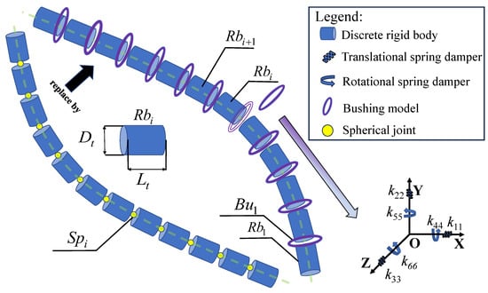
Figure 1.
Finite cylindrical rigid bodies and bushing forces for cable modeling.
Unlike spherical joints, which permit unrestricted rotation around a fixed pivot point, bushings provide elastic connections that allow limited rotations and translations. This characteristic more accurately reflects the continuous nature of the cable, especially when subject to bending forces caused by wind and other environmental conditions. The bushing model introduces elastic forces proportional to the relative displacements and velocities between adjacent cable segments, enhancing the system’s ability to handle large deflections and rotations. By redistributing internal stresses more evenly, this approach enables more precise simulation of the cable system’s response to external forces, particularly the complex aerodynamic effects experienced in tethered balloon applications.
The height of the tethered balloon was fixed at 600 m. This indicates that the cable is 600 m long overall. The tethered cables were connected to the balloon in an umbrella-like configuration, as shown in Figure 2. Specifically, the upper ends of the 12 cables were circumferentially fixed to anchor points at the bottom of the tethered balloon, while their lower ends were twisted together to form a single thick cable. The locations and directions of both cable ends, as well as the characteristics of the synthetic fiber, serve as the input parameters for geometric modeling. In the longitudinal plane of the tethered balloon, the X axis points in the direction from head to tail, the Y axis points in the direction of balloon rise, and the Z axis points in the direction of balloon yaw.
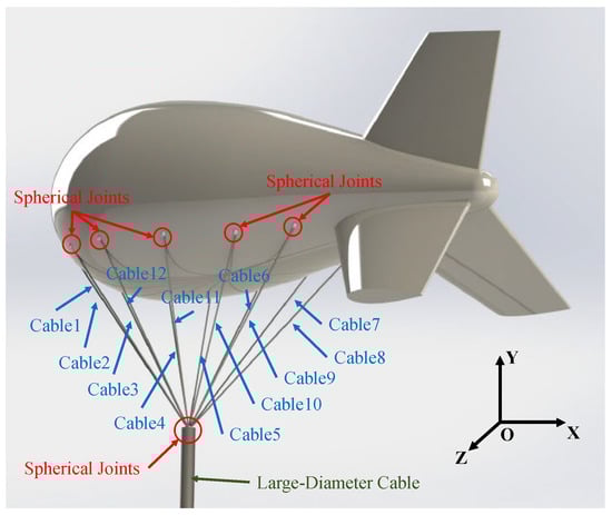
Figure 2.
Layout details of the tethered balloon cable system.
To preserve the flexible characteristics of the rope structure as much as possible while reducing computational costs [32], Huston’s discrete multibody system modeling method was employed for the cable system. The tether cable of the balloon was discretized into multiple small cylindrical segments, with each segment assumed to be a homogeneous rigid body, meaning no deformation occurs during motion. Additionally, to prevent separation between the balloon and the cables, spherical joints were added between the upper end of the cable and its attachment point to the balloon. As shown in Figure 2, the large-diameter tethered cable was connected to the balloon via 12 tethered cables, with the upper ends attached to the balloon through spherical joints. The lower ends converged into a single large-diameter cable. Similarly, for the sake of equivalence, the 12 cables were also connected to the thick cable below using spherical joints. A ball hinge pair connected the near-ground end of the cable to the ground. As was discussed in the preceding section, bushing models are used to replace spherical joints in order to compute the forces and torques acting on the rigid bodies. The details of the bushing force model are presented in Figure 1 in the form of a space spring. The translational and rotational springs on the three axes represent the translational and rotational stiffness of the bushing model on the three axes, respectively.
In accordance with the orientation depicted in Figure 2—serving as the direction of the global coordinate system—in the generalized Cartesian coordinate system, the generalized coordinates of any rigid body are determined by the coordinates of the origin of the floating coordinate system fixed to the body and the rotational angles that define the orientation of the floating coordinate system relative to the global coordinate system. The position and orientation of the rigid body can be expressed as follows:
The origin of the system’s absolute coordinate system is identified at point O, as illustrated in Figure 3, and the origin of the rigid body’s local coordinate system resides at the centroid of the body. In this figure, represents the position of point P in the global coordinate system, while r denotes the coordinate of the body coordinate system origin in the global coordinate system. The vector from the body’s origin to point P is denoted as in the global coordinate system. In Equation (1), the position vector of point P within the body coordinate system is represented as , and the Euler rotation matrix A is defined as follows:
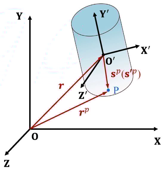
Figure 3.
Presentation of the reference frame.
According to Euler’s rotation theorem, the initial orientation of the floating coordinate system coincides with the global coordinate system. The orientation of the rigid body can be determined by the angles of rotation around the floating coordinate system’s own axis, axis, and then -axis again, following the common 313 rotation sequence. The rotation angles are denoted as , , and , respectively. Using the generalized coordinates to describe the position and orientation of rigid body i () in the global coordinate system, the first three terms of represent the position, while the remaining terms represent the rotation angles determined according to the 313 rotation sequence, and the description is as follows:
where represents the position matrix of the rigid body, and represents the Euler angle matrix of the rigid body. Similarly, the generalized force is used to denote the force and the torque experienced by , which are expressed by the following formula:
Considering all the rigid bodies as a whole, the generalized coordinate and the generalized force of the multibody system are composed of the subvectors and , respectively:
The cable system is divided into n segments: that means the whole cable system has 6n degrees of freedom. The kinematic equations of the entire system can be obtained through the application of the Newton–Euler theorem and the Lagrange multiplier theorem:
where M is the generalized mass matrix of the system, which includes the mass and the moment of inertia matrices of the system. r represents the generalized displacement matrix of the system, which includes both translational and rotational displacements of the system. And denotes the displacement and rotation constraints of the system.
The bushing models in the cable system are used to replace the spherical joints between discrete rigid bodies, which means that many constraint equations are transformed into the equation of force in the dynamics equations of the system. Furthermore, the remaining spherical joints are represented as constraint equations in the dynamics equations for linking the cable system to the ground and balloon. The dynamics equations of the discrete rigid bodies can be represented in two distinct forms in this scenario. The dynamics equations of the discrete rigid body (expressed as ), whose spherical joints are completely replaced by bushing models, are as follows:
where and represent the bushing forces and bushing moments, whose magnitudes depend on the displacements and rotations between adjacent rigid bodies. and are the external forces and torques. The dynamics equations of a discrete rigid body keeping a spherical joint (expressed as ) are as follows:
The generalized force and torque are delivered among rigid bodies by the bushing model, such as and in Figure 1 and Figure 4. We determine the external force and torque load on the cable system, and the changes the location and orientation of first; then, the bushing model generates the same effect on due to the displacement and angle variation of . The following equations define how the force and torque are transferred from the bushing model to the rigid bodies, depending on the displacement and velocity of the relative to .
where represents the relative displacement between adjacent rigid bodies in the global coordinate system, with its three directional components denoted as , , and . represents the relative rotation between adjacent rigid bodies in the global coordinate system, with its components denoted as , , and . In a system composed of adjacent rigid bodies, assuming that the floating coordinate system of and the global coordinate system are shown as Figure 5, the rotation matrix of relative to is defined as . According to Equation (1), can be obtained from the following expression:
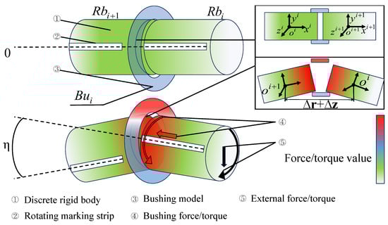
Figure 4.
The effects of bushing forces on two discrete rigid bodies.
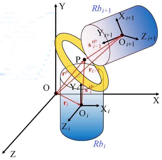
Figure 5.
Relative movement and rotation between rigid bodies.
K represents the stiffness matrix, where values from to represent the translational stiffness coefficients and rotational stiffness coefficients of the bushings in the global coordinate system along three directions. Similarly, C denotes the damping coefficients matrix of the bushing model.
The diagonal elements in matrix C are given by the empirical operation (1∼10 N·mm/s), and the elements in matrix K are calculated using Equation (13). The detailed action of the bushing force is shown in Figure 4. We considered the rigid bodies and , as well as the bushing forces between them, as a dynamic system. There was no relative displacement or relative rotation between the rigid bodies and in the previous iteration. At the current iteration step, the generalized force of the system is the resultant force of the external force and the bushing force. Under the action of the resultant force, rotates by an angle of , and the distance between the rigid bodies becomes + .
Figure 6 illustrates the constraint relationship between two rigid bodies interconnected by a ball–joint pair. Point P is the center of rotation for the spherical joint connecting bodies and . As a result, the global position vectors and of point P, located on both bodies and , coincide. and represent the vectors of point P in the floating coordinate systems of and , respectively.
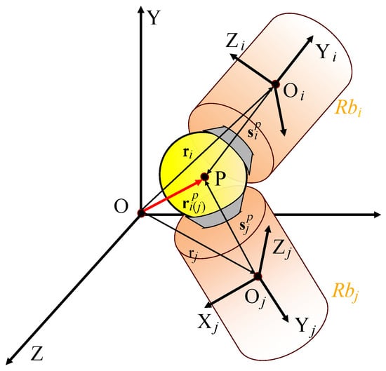
Figure 6.
The spherical joint constraint between two discrete rigid bodies.
Indeed, the bushing model has been encapsulated in various commercial multibody dynamics software. However, in this paper, we established the bushing model using the relative coordinate method and considered it as a flexible connection between adjacent discrete rigid bodies. The relative motion and the magnitude of the bushing force between adjacent bodies can be easily obtained from Equation (9). This is crucial for analyzing the motion response of long cable structures. Furthermore, the spherical joint permits only relative rotation amongst discrete rigid bodies, thereby allowing the constraint equations in Equation (8) to be presented as follows:
where and are the rotation matrices of and , respectively.
3. Tethered Balloon Dynamics and Wind Load Modeling
The balloon is regarded as a rigid body, and the pressure regulation system ensures that its volume shape is unchangeable. As shown in Figure 2, in this study, the X axis is defined as the direction from the front (nose) of the balloon to the rear (tail), with the Y axis being the positive vertical direction in which the balloon ascends. The Z axis is defined as the lateral direction. The balloon is symmetric along both the XY and XZ planes. The balloon mass and its center of gravity remain unchanged. The volume center of the balloon coincides with the center of gravity. The ground frame is approximated by an absolute inertial frame. The density of the earth atmosphere varies with height. The atmospheric density around the balloon is normally considered to be approximately uniform in solving the problem of balloon dynamics.
The dynamics of the tethered balloon and the discrete rigid bodies in the system can be described using three primary angular motions: pitch, yaw, and roll. The pitch angle describes the rotation around the Z axis (longitudinal axis). The pitch angle changes when the balloon tilts up or down, and it is mainly influenced by the aerodynamic lift and pitch moment. The yaw angle describes the rotation around the Y axis (vertical axis). It is affected by lateral aerodynamic forces, particularly the side force and yaw moment, causing the balloon to rotate in the horizontal plane (i.e., deflecting left or right). And roll angle describes the rotation around the X axis (lateral axis). The roll angle is driven by the roll moment, especially when the balloon experiences lateral instability or asymmetric aerodynamic forces.
The Reynolds number, air density, temperature, and fluid viscosity are all physical factors that have an impact on the aerodynamic force and the extra inertia force. It is undoubtedly a difficult task to include the aerodynamic elements in this paper. As a result, the modeling of the added inertial force and the aerodynamic force was simplified in this work. The computation was based on the experimental data fit and pertinent national standards. This paper considered the tethered balloon as a rigid body. Accordingly, based on Equation (6), the dynamic model of the tethered balloon is defined as follows:
The centroid of the balloon’s shape is considered as the origin of its floating coordinate system when establishing the dynamic equations of the tethered balloon. In Equation (15), represents the mass matrix of the tethered balloon, represents the inertia matrix of the tethered balloon, represents the position of the balloon’s floating coordinate system origin in the global coordinate system, represents the geometric constraints of the balloon connected to the tether by spherical joint pairs, represents the forces acting on the balloon, represents the torque acting on the balloon, and represent the forces and torques exerted by the airflow on the balloon, and represent the forces and torques exerted by the cable system on the balloon, represents the buoyancy force of the balloon itself, and denotes gravity. represents the initial torque of the balloon, which exists because the center of gravity and the center of buoyancy of the balloon are not in the same position.
Due to the tethered balloon being connected to the cable system via spherical joint pairs, there are no constraints on the rotation in the dynamic equations. Considering only aerodynamic lift, aerodynamic drag, and aerodynamic pitching moments, and can be calculated using the following set of equations:
where, , , and represent aerodynamic lift, aerodynamic drag, and aerodynamic pitching moments acting on the balloon; , , and , as well as , , and , represent, respectively, the additional mass forces and additional inertia torques of the tethered balloon in three directions of motion and rotation. Their calculation formulas are as follows:
where , , and represent aerodynamic lift coefficient, aerodynamic drag coefficient and aerodynamic pitch moment coefficient, respectively. represents the air density, denotes the air flow speed (i.e., wind speed), refers to the reference area of the balloon, and is the characteristic length of the balloon. and express the additional mass coefficient matrix and additional rotational inertia coefficient matrix of the balloon, respectively. The additional mass coefficients and additional rotational inertia coefficients of the tethered balloon on the three coordinate axes are shown in Table 1. It is worth noting that due to the symmetric properties of the tethered balloon, its additional rotational inertia coefficient in the X-axis direction is very small and can be neglected in the calculation process. What is more, the negative sign preceding the additional inertial forces and torques indicates that their direction is opposite to the direction of motion of the object.

Table 1.
Additional inertia force coefficient.
Figure 7 illustrates the fitting of the aerodynamic coefficients corresponding to the lift, drag, and pitching moment. The discrete points represent the experimental data for the three parameters, while the solid lines are quadratic polynomial fits derived from the experimental data and the tethered balloon’s pitch angle , as expressed in Equations (19)–(21). The fitting results show a good correlation between the curves and the experimental data, with correlation coefficient values of 0.996 for the equation, 0.988 for the equation, and 0.944 for the equation. In the following analysis, the fitted equations will be directly used to reduce the number of parameters in the dynamic equations of the system.
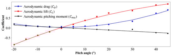
Figure 7.
Fitting of aerodynamic coefficient functions.
Substituting Equations (19)–(21) into Equation (18), the following equation can be obtained for computing the aerodynamic forces and moments:
The overall impact of aerodynamic forces on the tethered cable can not be overlooked. The outer surface of the cable serves as the location where aerodynamic forces act. When the cable moves under the influence of airflow, the aerodynamic forces it experiences are primarily considered as the combined force of aerodynamic drag and additional mass forces . Treating the aerodynamic forces acting on the discrete rigid bodies of the tethered cable as external forces, denoted as , the calculation formula for in Equations (7) and (8) is as follows:
where is the cable aerodynamic drag coefficient, and represents the corresponding area. represents the additional mass force of the discrete rigid body of the cable in the X-axis direction, and is the additional inertia coefficient matrix of the cable.
The tethered balloon works in the troposphere at 600 m above the ground. The wind speed varies as a function of the height. The wind profile model with respect to the height is therefore described as follows:
where h represents the height, and is the friction velocity, which refers to a parameter used to describe turbulence and friction effects near the Earth’s surface. represents the von Karman constant, which was set to 0.4 in this work. It is worth noting that represents the ground roughness length when the height above ground is 10 m. When the height is less than 10 m, the original ground roughness length becomes ineffective. Therefore, in Equation (24), the wind profile model is divided into two parts. When the height is below 10 m, the wind speed value at the height of 10 m is taken as the wind speed of the wind profile. And can be calculated by assuming the Charnock constant:
where represents Charnock constant, which was set to 0.014 in this work. was regarded as 0.4186 m/s.
By substituting Equation (25) into Equation (24), we obtain the following equation to describe the wind profiles:
Taking into account that the troposphere is 600 m, the tethered balloon rarely operates at more than 35 m/s. Thus, the working environment of the balloon was set below 35 m/s. Equation (26) was used to calculate the wind speed, whereas the gust model was not considered. We will explain the gust model as an external boundary condition in the next section.
4. Simulation Results
The near-surface troposphere presents a more challenging air flow scenario, making it difficult for tethered balloons used for scientific observation. As a result, the dynamic responses of the tethered balloon were examined in three different scenarios: one in which the balloon only encounters a steady wind, another in which the balloon and cable are subjected to wind profiles, and a third in which the wind profiles and gusts are coupled. The wind model taking into account the wind profiles, and gusts are defined as follows:
where represents the gust wind speed; it is artificially divided into two cases. The second case is a constant-speed gust with a wind speed of 10 m/s and a duration of 60 s. However, when incorporating a constant gust model into the system, it is necessary to use the STEP function to describe the process of wind speed increase. When the gust model is a constant gust, can be represented by the following equation:
where the STEP function is an approximation of the Heaviside step function using a cubic polynomial, indicating that the process of gust wind speed increase is gradually achieved to 10 m/s through a cubic polynomial, rather than abruptly changing to 10 m/s. Subsequently, the wind maintains a constant speed of 10 m/s until 62 s, and then it decreases back to 0 over the next 2 s starting at 62 s. The entire gust duration lasts 64 s, with the effective wind speed of 10 m/s acting for 60 s. The purpose of introducing a constant gust is to assess the impact of gust loads on the system’s dynamic response. In the second case, the gust wind speeds follow a normal distribution of . A scaling factor of 25 is chosen to ensure that the wind speed approaches 10 m/s when the simulation time is close to 30 s. When the gust model is a constant gust, can be represented by the following equation:
The introduction of normally distributed gusts aims to simulate the stability of the system in a realistic wind field environment. The critical parameters of the tethered cable–balloon system are listed in Table 2.
Table 2.
Critical parameters of the tethered cable system.
In this work, is used to denote the effective length of balloon, and the balloon-related parameters are listed in Table 3. The wind loads mentioned above are applied to the center of mass of the tethered balloon and each discrete segment of the cables, acting in the positive X direction of the global coordinate system (with the balloon’s front facing the wind). Other external forces and moments, such as gravity, buoyancy, aerodynamic forces, cable tension, and associated moments, are applied to the center of mass of the tethered balloon body.
Table 3.
Critical parameters associated with the balloon.
4.1. Comparison of Different Cable Modeling Methods
In the second part of this paper, a detailed description of the dynamics model of the cable system is provided. However, for the evaluation of a new modeling approach, it is essential to compare it with the currently popular methods. Therefore, we utilized the same cable model and employed the finite element method (FEM), computational fluid dynamics (CFDs), rigid bodies with the spherical joint method, and rigid bodies with the bushing method for modeling. We conducted a comparative analysis of the physical quantities related to motion and force in the cable system under the same external loads. This comparison aims to evaluate the effectiveness of the proposed modeling method in this paper.
The physical model used for comparative simulation consists of a cylindrical cable with a length of 100 m and a radius of 0.1 m. Its bottom end is fixed to the ground, as depicted in the schematic diagram shown in Table 4.
Table 4.
Simulation results of different modeling methods.
The applied force on the physical model is a distributed force along the X axis with a magnitude of 10 kN. It is important to note that, in the CFDs method, to ensure consistency with the external loads applied in the other three models, in addition to setting the fluid flow velocity, compensatory forces in the same direction need to be applied on the surface of the physical model. This is done to ensure that the resultant force from the compensatory forces and the air flow acting on the cylinder approximate 10 kN. In the simulation result images shown in Table 4, for the cylinder fixed on the ground and subjected to the same distributed force, the deformations of the models using different modeling methods are not entirely identical. The models using the CFDs method and the rigid bodies with the bushing method exhibited smaller deformations, with an overall inclination consistent with the direction of force. However, the model constructed using the finite element method showed a significant bending deformation at one end of the cylinder, where it hung freely, with stress concentrated near the hanging end. On the other hand, the model established using rigid bodies with the spherical joint method underwent bending at the fixed end, with the direction of bending opposite to the direction of force application. This characteristic resembles more of a chain-like structure than the cable structure.
Here, we have selected the velocity along the X axis, axial force, and constraint reaction force of the cable as the objects of comparative analysis. represents the axial force, denotes the velocity of the cable along the X axis, and and are the constraint reaction forces of the fixed joint along X and Y axis, respectively. The comparative results are as follows:
The results presented in Figure 8 compare four different modeling methods used to evaluate the dynamic response of a cable system. The methods analyzed include the CFDs method, the FEM, the spherical joint method, and the discrete rigid body–bushing force method. The results highlight significant differences in the predictive performance of these models concerning the dynamic characteristics of the cable system. First, the FEM results exhibited a distinct divergence after 0.1 s, indicating that this method is not suitable for modeling the cable system when large displacements and rotations occur. The FEM struggled to produce accurate and stable results under significant deformation and motion, making it an unfavorable choice for dynamic evaluation of the cable system.
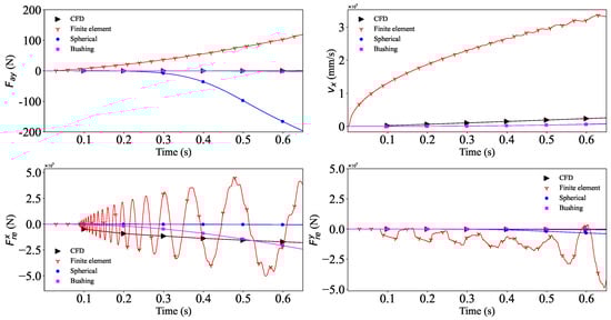
Figure 8.
Comparison of results among different modeling methods.
Second, the spherical joint method showed an unrealistic early increase in axial force. This phenomenon arose from the fact that, after displacement, the rigid bodies connected by spherical joints could not rotate freely, causing abnormal axial force accumulation. This behavior can lead to overstressing the cable, potentially resulting in breakage as the axial force exceeds the tensile strength limit. On the other hand, the spherical joint method is also not ideal for modeling large-deformation cable systems. In contrast, the discrete rigid body–bushing force method demonstrated results that closely align with the CFDs method, and the numerical values remained relatively stable. This indicates that the discrete rigid body–bushing force method effectively handles large-scale cable motion and rotation with greater computational efficiency.
Additionally, the CFDs method, which accounts for complex factors such as airflow and cable stress–strain behavior, serves as a valuable reference for assessing the dynamic characteristics of the cable system, despite its higher computational cost. Therefore, the discrete rigid body–bushing force method proved to be an effective approach for modeling the tethered cable system under large displacements and bending deformations, making it a suitable choice for this study.
4.2. Dynamic Response Comparison with CFDs Benchmark
In the previous section, the effectiveness of modeling using the bushing model was evaluated through comparisons with different modeling approaches, and it was found that the CFDs and the rigid bodies with bushing modeling methods exhibited similarity in the simulation results. To further assess the accuracy of the system modeling, in this section, we employed the same balloon model and conducted motion response analysis using both the CFD and multibody system dynamics methods. The results obtained from the CFDs method were taken as the benchmark to evaluate the accuracy of modeling the balloon. Additionally, we conducted a comparative analysis of the motion response of the entire system using the rigid bodies with spherical joint method to further validate the accuracy of the bushing method and highlight its advantages. The comparison parameter is the pitch angle of the tethered balloon, as shown in Figure 9.
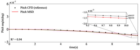
Figure 9.
Results comparation between CFDs and MSDs.
The difference in the tethered balloon pitch angle between the two methods is minuscule, with a deviation of 0.0016° at 10 s, as shown in Figure 9. Taking the results in the CFDs method as the reference and the results in the multibody system dynamics (MSDs) as the data for the fit, we use the value to illustrate the degree of fit of the two groups of data. The value is closer to 1, indicating that the two groups of data fit better. This comparison tested the effectiveness of tethered balloon modeling in multibody dynamics methods. Additionally, compared to the MSDs method under the same conditions, the CFDs method required significantly more computational resources. Specifically, under the same computing setup (workstation simulation platform: Intel(R) Xeon(R) Gold 6248R CPU @ 3.00 GHz, 48 cores; system platform: Windows 10 Professional; CFD simulation platform: Ansys; MSD simulation platform: Adams), the CFDs method took 48 min to solve, whereas the MSDs method only took 10 min. This indicates that the MSDs method improved the computational speed by nearly 80%, with minimal differences in the results. The reason for this is that the CFDs simulation accounts for detailed factors such as the balloon’s surface stress and strain variations, pressure characteristics, and airflow around the balloon. The CFDs method involves meshing both the balloon and the external flow field, resulting in a larger number of mesh elements. In contrast, the MSDs method simplifies the balloon as a rigid body, avoiding the need to compute surface stress and strain parameters, which are not the focus of this study.
What is more, in the cable system, the bushings model was used to replace spherical joints model for connecting rigid bodies. In order to verify the effect of the bushing force model, we analyzed the force of the bushing model and spherical joints model at the rigid body connection under the same conditions, as shown in Figure 10. represents the number of i spherical joints connecting and , exactly as shown in Figure 1.
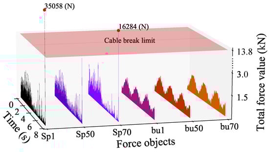
Figure 10.
Total force on different objects.
In Figure 10, the red plane represents the tensile strength limit of the cable, which is 13.8 kN. This indicates that if the axial force calculated in the cable model exceeds this value, there is a significant risk of cable failure. This figure clearly shows that the actuation forces of the spherical joints among the rigid bodies rose steeply after the 7th second, and they exceeded the plane of failure of the cable, resulting in failure of the resolution. This phenomenon is due to the fact that the cable system connected by spherical joints has fewer degrees of freedom than when it is connected by the bushing model.
As the cable system bends due to the action of an external force, the force among discrete rigid bodies will build up at a portion of the joints, causing the abnormal connective force to increase. This conclusion is consistent with earlier findings, further confirming that the rigid body of the spherical joint method is not suitable for the cable model proposed in this paper. While the spherical joints model computed slightly faster than the bushings model, these anomalies still limit its utility as a connection method for multi-rigid-body cable systems. After comparing the modeling methods, the next step is to evaluate in detail the performance of tethered balloons under different working conditions and modeling settings.
4.3. Dynamic Responses under Steady Wind
Analyzing the motion response of a tethered balloon system is a key step in assessing its wind resistance capabilities. The tethered balloon system consists of cables and a balloon connected by spherical joints; thus, the analysis focuses on the balloon sphere and the discrete rigid bodies that make up cables. Within the system, forces on the cable are transmitted through the kinematic pair, resulting in visible changes in the attitude of the tethered balloon. Therefore, the balloon’s attitude is considered the primary parameter for assessment. Additionally, to grasp the forces and torques on the cable, an evaluation of the forces acting on the discrete rigid bodies will also be conducted.
First, the dynamic response of the tethered balloon system was evaluated by dynamic simulations under steady wind profiles. For clarity, this scenario is referred to as Case A throughout the study. The wind speed on the balloon part was set at 15 m/s for 155 s. The displacement of the balloon along its three axes, or its angles of pitch, roll, and yaw, are the primary responses that need to be examined. It is evident that the choice of the aforementioned parameters can effectively characterize the dynamic reactions of the tethered balloon, despite the fact that a large number of factors can reflect the performance of the tethered balloon. It should be noted that cable segment heights are sorted in this section. The numbering begins close to the tether of the balloon and comes to an end not far from the surface.
Under the influence of a constant wind of 15 m/s in the positive X direction, the overall dynamic response of the system is evaluated. As shown in Figure 11a, the tethered balloon oscillated back and forth along the X axis with a period of 100 s, reaching a maximum displacement of 134.4 m. Due to the constraints imposed by the tether, the balloon also underwent vertical oscillations along the Y axis, with a maximum displacement of 18.3 m during the same 100-s period. In the Z direction, there was minimal movement, as there was no lateral wind influence. These observations align with the expected response.
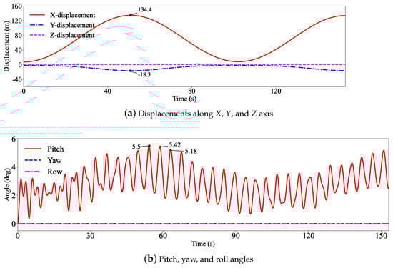
Figure 11.
The displacements and angles of the tethered balloon under steady wind.
Figure 11b illustrates the rotation of the tethered balloon around the X, Y, and Z axes. Due to the connection between the main tether and the balloon via 12 tether cables in an umbrella-shaped configuration, the balloon experienced rotational motion during its oscillation. As expected, the tethered balloon exhibited periodic pitching motion around the Z axis, with a period of 100 s and a maximum pitch angle of 5.5°. This was accompanied by oscillations with an amplitude of approximately 2°, which is attributed to the use of the bushing force model that accounts for the elastic forces in the cable. The yaw and roll angles around the Y axis and X axis, respectively, exhibited only minor fluctuations around 0°, as there was no lateral or gust wind acting on the system. The results also indicate that the closer the tether segment is to the balloon, the greater the displacement variation and the smaller the angular change. Additionally, the overall bending of the tether system was minimal, approximating the behavior of an elastically supported beam structure.
4.4. Dynamic Responses under Wind Profiles
The dynamic responses of the tethered balloon system were easy to calculate when only considering the steady wind load in Case A. However, under more realistic conditions, the tethered balloon and cables operate under varying wind profiles. To simulate these conditions, a wind profile model was employed to evaluate the external wind load, which is referred to as Case B. In this case, the wind profile model (Equation (26)) introduces a variation in wind speed with height, applying external loads to the tethered balloon as defined in Equation (18) and to the cable segments according to Equation (23). The displacements and angles (pitch, yaw, and roll) of the tethered balloon are measured during a 100 s dynamic simulation process, as shown in Figure 12.
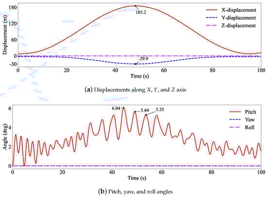
Figure 12.
The displacements and angles of the tethered balloon under wind profiles.
As shown in Figure 12a, the results indicate that under the influence of the wind profile, the tethered balloon underwent periodic motion along both the X and Y axes with a cycle period of 96 s while exhibiting negligible lateral displacement. The balloon moved periodically along the X axis, reaching a maximum displacement of 185.2 m, while along the Y axis, the maximum displacement was 29.9 m. This movement was caused by significant motion in the direction of the wind speed, particularly in the central section of the tethered cables. The increased cable stress resulted in the descent of the tethered balloon. Once the tension in the central section of the cables began to relax slowly, the balloon’s the buoyant force became greater than the cable tension, causing the entire balloon system to ascend. As the balloon rose, the cable tension gradually increased again, leading to periodic motion until dynamic equilibrium was reached between the cable tension and balloon’s buoyancy.
Figure 12b shows the variations in pitch, yaw, and roll angles over time. The pitch angle underwent periodic fluctuations with minor oscillations, reaching a maximum Z axis deflection of 6.04° due to the constraints of the tethered cables and the influence of the wind profile, with subsequent oscillations gradually diminishing. However, the yaw and roll angles remained nearly constant around 0° throughout the simulation. This confirms the conclusion from the previous case, where the wind blowing along the X axis primarily affected the pitch angle, with minimal impact on the yaw and roll angles.
4.5. Dynamic Responses under Wind Profile and Gust Wind
The wind profile model is often used to represent the average wind speed over a period of time. That is, the wind speed does not change with respect to time. Because the tropospheric air velocity changes not only in height but also in time, a discrete gust was additionally introduced to combine with the model of the wind profiles in this section. Suppose an additional gust with a constant velocity of 10 m/s occurs at 300 to 600 m above the ground for more than 60 s; thus, the gust model (Equation (28)) proceeds as follows. The gust wind starts at 2 s and ends at 62 s during the dynamic simulations. The dynamic responses of the tethered balloon under a gusty wind model can clearly illustrate the influence of uneven flow on the tethered balloon. The dynamic responses in this case are critical to evaluate the wind resistance of the tethered balloon. Similarly, the displacements and angles of the tethered balloon are used as key parameters to describe the motions of the tethered balloon system. This situation is defined as Case C.
The gust model was created according to Equation (27). Figure 13a,b depict the displacement and orientation of the tethered balloon in Case C. Based on the analysis of previous cases, applying wind loads solely in the X direction did not affect displacement along the Z axis. Therefore, Figure 13a only illustrates the displacement along the X axis under wind profiles with and without additional gusts, as well as the Y-axis displacement when gust loads were considered. The additional gust load increased the maximum X-axis displacement of the tethered balloon from 185.2 m (without gusts) to 203.4 m, yielding an increase of 18.2 m. The red shaded area in the figure highlights this difference. Figure 13b shows the difference in pitch angle between the scenarios with and without gusts, which is also indicated by the red shaded area. Similarly, the additional gust load increased the pitch angle of the tethered balloon, with the maximum pitch angle increasing by 0.55° from 6.04° (without gusts) to 6.59° when gusts were included.
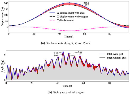
Figure 13.
The displacements and angles of the tethered balloon under wind profile and gust wind.
In real-world conditions, gust increases and decreases are not abrupt; given a sufficient number of samples, the variation in gust wind speed typically follows a certain distribution pattern. This gust model is markedly different from a constant gust model. Based on Equation (27), an alternative gust model (a normally distributed wind with N (30,1) characteristics, Equation (29)) was applied to the entire system, defining this scenario as Case D. By comparing Case D with Case C, this scenario was developed. The stability of the tethered balloon system under more realistic environmental conditions was assessed. Figure 14 illustrates the performance of the discrete rigid bodies within the cable section of the tethered balloon system under different gust models. The investigation focuses on a discrete rigid body located in the middle of the cable, evaluating the forces along the X and Y axes, the torque around the Z axis, and the displacement along the X axis. Among these, the force along the Y axis corresponds to the axial force on the cable.
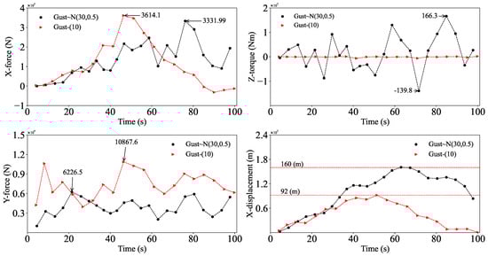
Figure 14.
The impact of varying gust models on cables.
Figure 14 shows that under the constant gust model (Guest∼(10)), the forces along both the X and Y axes experienced by the discrete rigid body were significantly larger than those under the normal distribution gust condition (Guest∼N (30, 0.5)). Additionally, the torque around the Z axis was consistently greater throughout the simulation in the normal distribution gust scenario, indicating that the normal distribution gusts are more likely to cause bending of the cable around the Z axis. This corresponds to the increased X axis displacement observed in the tethered balloon under the normal distribution gust model. Moreover, the axial force results in the Y direction indicate that under a sustained constant gust, the cable experienced a much larger axial load (up to 10,867.6 N), which could potentially lead to cable failure. In contrast, under the normal distribution gust model, the variation in axial force was more stable. The force along the X axis behaved differently. After 64 s, when the normal distribution gust dissipated, the X-axis force acting on the balloon continued to oscillate and increase, indicating a higher likelihood of system instability and failure due to attitude anomalies. On the other hand, under the constant gust conditions, the X-axis force gradually decreased, reducing the risk of system failure.
To quantitatively analyze the impact of environmental changes on the dynamic responses of the tethered balloon system, the main responses in these four cases have been compared. The information about the displacement, attitude angle, and bushing force and torque of cable segments under the above cases are depicted in Table 5.
Table 5.
Main parameters in four cases.
It can be seen that the overall displacement of the tethered balloon system under the action of wind profile increased by 32.3% compared to the result under the action of steady wind. The roll and yaw angles increased inconspicuously under the wind profiles. When considering the tethered cable load, the tethered balloon dropped downward due to the increase in cable forces.
By comparing the results with and without gust wind, it can be seen that the air velocity is the key factor affecting the dynamic responses of the tethered balloon system. Furthermore, the gust wind increased the pitch movement of the tethered balloon, and the displacements between discrete rigid bodies became greater, which is more likely to lead to cable failure. The greater the pitch displacement is, the larger the roll and yaw motions of the balloon are due to the special funnel cable structure connected to the balloon. The balloon is more susceptible to rolling and capsizing when considering the big change in pitch angle.
Upon comparing Case D with Case C, it has been discerned that a normal distribution gust model precipitates a more pronounced oscillation of the cable system, surpassing that induced by a constant gust model. Furthermore, as the oscillations of the cable system intensify, there is also a marked increase in the variation of the tethered balloon’s attitude. Under a constant gust environment, the forces acting upon the discrete rigid bodies were conspicuously greater than those in a normal distribution gust environment. In summary, under the normal distribution gust model, the torque on the discrete rigid bodies escalated, augmenting the swaying of the cable system and rendering the system susceptible to attitude anomalies and consequent failure. Conversely, under the constant gust model, the forces exerted on the discrete rigid bodies were amplified, increasing the axial force on the cable and predisposing the system to the likelihood of rope breakage and failure.
5. Discussion
In the above sections, a three-dimensional model of the tethered cable system was established, and the overall dynamic response of the system was evaluated by analyzing the three situations. The validity of the model of replacing the ball–hinge pair with the bushing force has been verified. In addition, it is significant for assessing the dynamic response of tethered balloons to evaluate the influence of the number of tethered cable segments on the dynamic response of the system, the impact of external wind load on different parts of the tethered cable on the overall motion response of the system, and the effect of the lateral wind on a tethered balloon. In this section, we will analyze and discuss the above problems in detail to describe more parameters that affect the normal operation of the tethered balloon. The discussion of these problems fully applies the established model to the three-dimensional scene and considers the performance of the model. The discussion in this part can provide valuable advice and experience for the correct establishment of a dynamic model of tethered balloons.
5.1. The Number of Cable Segments
From the analysis in the previous sections, it can be concluded that both the spherical joint modeling method and the discrete rigid body–bushing force modeling method can describe the rotational motion between adjacent discrete cable segments. Therefore, in scenarios involving small tensile loads on the cable, these two methods can be considered equivalent and interchangeable. However, the ideal spherical joint does not allow for deformation, which means that under large tensile loads, this method cannot accurately capture the elastic stretching characteristics of the cable. In contrast, the bushing force model allows for more flexible and elastic connections, better capturing the continuous bending and stretching behavior of a cable under external forces. Consequently, this study further investigated the effect of the number of discrete segments in the discrete rigid body–bushing force model on the accuracy of dynamic simulations of a tethered balloon system.
The tethered balloon system in this study included a 600-meter-long tether cable, which was discretized into 220, 320, and 420 segments of rigid bodies for analysis. The segment models have different lengths but the same radius. In the comparative simulation, the total simulation time was set to 100 s with a time step of 0.01 s, and the external loads included aerodynamic forces, additional inertial forces, and wind profile effects. Since the balloon’s attitude and displacement directly reflect the system’s dynamic response, the X-axis displacement, Y-axis displacement, and pitch angle of the balloon were selected as key metrics for comparing simulation accuracy. The maximum and average values of these motion characteristics from the simulation results are summarized in Table 6.
Table 6.
Effect of number of cable segments.
The data set is expressed by a violin diagram in Figure 15, which describes the data distribution of the displacement and pitch angle during the simulation process. As shown in Table 6 and Figure 15, the number of cable segments had a negligible influence on the balloon’s displacement along both the X and Y axes. Specifically, the relative change in displacement between models with 320 and 420 cable segments was only 0.5% the for X-axis displacement and 1.5% for the Y-axis displacement, highlighting that the translational movement of the balloon remained largely consistent regardless of the number of segments.
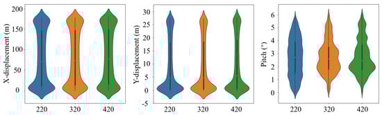
Figure 15.
Violin plot of data set under different number of cable segments.
However, the number of cable segments significantly impacted the pitch angle of the balloon. Figure 15 clearly shows that the time-series data for the pitch angle distribution diverged across the different models. The 220-segment model exhibited a narrower spread, indicating rapid changes in the pitch angle, while the 320- and 420-segment models displayed longer periods of stability at pitch angles of 1–2°. This suggests that while the 220-segment model responded quickly to external forces, it may also be more prone to instability or failure under larger external loads due to faster pitch angle variations. In contrast, although the 420-segment model demonstrated greater flexibility, it also took longer to stabilize back to a smaller pitch angle, as indicated by the concentration of data around higher pitch angles in Figure 15. This prolonged period at larger pitch angles increases the likelihood of abnormal balloon attitude, particularly under higher loads. Therefore, it is critical to strike a balance in selecting an appropriate number of cable segments. A model with too few segments may be overly stiff, leading to rapid changes in attitude and potential instability, while too many segments may lead to prolonged recovery times at higher angles, increasing the risk of system failure. This is the reason that the 320-segment cable MSD-model will be used in the following simulation research.
5.2. Different Parts the Gust Act
The gust model only considered the interval of 300–600 m in Section 4, that is, the dynamic response under wind acting on the upper part of the cable. However, it is natural that the gust generated in the near-surface troposphere can be artificially regarded as randomly appearing in any height range. Here, we only set the gust height directly (the wind speed is still 10 m/s and the duration is 60 s) and applied it to the upper part of the cable (300–600 m), the middle part (150–450 m) and the bottom part (0–300 m), respectively, to evaluate the performance of the system.
Table 7 shows the maximum value and mean value of the displacement along X axis, the displacement along Y axis, and the pitch angle of the tethered balloon under wind acting on different parts of cable. The data set is expressed by a violin diagram in Figure 16, which describes the data distribution of displacement and pitch angle during the simulation process. It can be seen from Figure 16 and Table 7 that the displacement and angle of the tethered balloon will be greater than it would be in other situations when the wind acts on the top of the cable. These results indicate that the ability to withstand wind at the bottom of the rope is stronger than it at the top of the rope in the tethered balloon system. The phenomenon is also valuable for designing tethered balloons that work at higher altitudes. When the tethered balloon is operating at a higher altitude, the effect of wind on the tethered line will be greater, which means that additional measures are needed to strengthen the stability of the tethered balloon. Several methods are listed that include increasing the buoyancy of the tether ball, adding auxiliary buoyancy equipment in the middle of the cable, and using better materials to reduce the diameter of the rope. But increasing the buoyancy of the balloon and increasing the amount of auxiliary buoyancy equipment also increases the work load, which is a further optimization issue. High-performance materials are also expected to be the key to the height of tethered balloons.
Table 7.
Influence of wind acting on different parts.
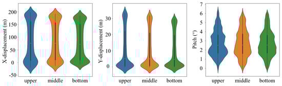
Figure 16.
Violin plot of data set under wind acting on different parts.
5.3. The Directions of Gust
Section 4.3 is an evaluation of the dynamic response characteristics of the tethered balloon system under a gusty wind with no deflection, which is applicable to the two-dimensional model. However, the construction of a full three-dimensional model requires consideration of wind direction as a factor that shows the variation in the performance of the tethered balloon. Therefore, we fixed the direction of the gust, including the gust deflection of −20°, −10°, 10°, and 20°. Since the tethered balloon structure is symmetrical about the plane, we only counted the data sets under 10° deflection, 20° deflection, and no deflection, as shown in Figure 17 and Table 8.
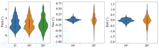
Figure 17.
Violin plot of data set under different wind direction.
Table 8.
Impact of wind direction.
Table 8 shows the maximum value and mean value of the pitch angle, yaw angle, and roll angle of the tethered balloon under gust acting in different directions. The data set is expressed by a violin diagram in Figure 17, which describes the data distribution of pitch angle, yaw angle, and roll angle during the simulation process. Due to the fact that the maximum yaw and roll angles of the balloon were less than 0.001° under the influence of gusts at a 0° deflection angle, they are not displayed in the violin plot of Figure 17. From the figure and the table, it can be observed that the direction of the gust significantly affected the pitch, yaw, and roll angles, with the latter two being particularly impacted. When the gust deflection angle increased to 10°, the maximum changes in the yaw and roll angles reached 0.24° and 0.45°, respectively. As the deflection angle increased further to 20°, their maximum angles nearly tripled, reaching 0.65° and 1.4°, respectively, though their average angles remained nearly unchanged, indicating that the tethered balloon oscillated around its initial position and that the oscillations became more intense as the gust angle increased. This phenomenon could be explained by the fact that when a deflected gust acts on a cable and causes it to move in the direction of the wind, the physical properties of the cable, combined with modeling inaccuracies, result in vibrations. These vibrations accumulate along the cable and are transferred to the tethered balloon, leading to additional yaw and roll motion.
5.4. Limitations of Simulated Motion
It can be seen from the Case D that there will be mutation points in the X and Y directions. This point is caused by the limited length of the cable and the connection with the ground by the ball joint. The energy is transferred between the balloon and the discrete rigid body of the cable in the form of waves. This is particularly evident in the displacement diagram. There are abrupt turning points at the last stages of the balloon descent and recovery. When the external loading conditions are further extended to more than three times the usual range, the large displacement at the turning point will cause the balloon to capsize. A common measure is to increase the buoyancy of the balloon to enhance the tightness of the cable to resist the influence of external load, but this measure obviously needs to increase the work load of the balloon. The ground-tethered equipment endowed with a certain buffer device can slow down the occurrence of such phenomena, wherein a method with buffer characteristics and less freedom of the restraint cable is desirable.
Incidentally, the modeling method proposed in the manuscript incorporates a six degrees of freedom framework that, while representing the most generic case theoretically, also introduces certain perplexities. The arduous nature of solving equations manifests when the chosen materials exhibit either infinitesimal or infinite resistance in particular orientations. This implies that the application of materials with such characteristics within a cable system may, when utilizing the bushing method outlined in this paper, give rise to issues of computational inefficiency.
Additionally, in the process of balloon modeling, the aerodynamic force only considers the aerodynamic lift, aerodynamic drag, and aerodynamic pitch moment in the plane, which is far from enough for complete aerodynamic modeling. The aerodynamic yaw moment, the aerodynamic roll moment, and the force generated by the side wind of the balloon will have a certain impact on the balloon. More data will establish a more durable and stable balloon model. However, according to the existing research results, there is a lack of data in this respect, and comprehensive CFDs calculations and wind tunnel tests are necessary for tethered balloon modeling. The wind profile used in this paper is only a statistical near-surface wind profile model. In fact, the height of tethered balloon theory can far exceed this limit, and it seems feasible to fit the wind profile model with relevant meteorological bureau information. The development of a stratospheric-related wind profile or airflow will bring new possibilities for tethered balloons.
6. Conclusions
The purpose of this paper was to use a new equivalent method to model a tethered balloon cable structure based on multibody dynamics, and the entire tethered balloon system was modeled by combining the relevant aerodynamic parameters and wind data. Based on this, the model was simulated, and its motion-response characteristics were estimated. In addition, the correctness of the modeling method was verified, and some interesting results were obtained. Coupled with an improved model, some research has been done on the motion response characteristics of a tethered balloon system, and a few crucial results have been obtained. Although the attached research setup conditions are relatively simple, they can still accurately reflect the influence of some external environmental factors on the overall motion response characteristics of a tethered balloon system, as well as the changing tendency of the system. From the above assessment of the motion characteristics of the tethered balloon system, the following conclusions can be drawn:
- -
- Compared to the CFD method, the balloon model established by the MSDs method had an 80% reduction in solution time with a difference of 0.0016° in pitch angle. The use of bushing models instead of spherical joints significantly reduced the force between discrete rigid bodies to a level below the maximum capacity of a cable. The results show that multibody system dynamics are more efficient and faster than other methods in dealing with the performance evaluation of objects.
- -
- The position and condition of a tethered balloon can be significantly affected or even dominated by the load carried by the cable at work. Thus, the cable load must be considered when modeling a tethered balloon system. The longer the tether and the greater the height of the tethered balloon, the more obvious the proportion of cable loading will be. The number of cable segments connected by the bushing force directly affects the characteristics of a flexible body and a rigid body. The appropriate number of segments established in this paper was controlled to be 0.3–0.5% of the total length of the cable for each segment of a discrete rigid body, that is, 320 segments. The characteristics of a flexible cable body may be more accurately reflected in this range.
- -
- The position and direction of the wind will have a great impact on the performance of the system. This is reflected in the effect of wind acting on the upper, middle, and bottom part of the cable, wherein the pitch angle and displacement of the balloon will change. The wind direction directly affects the posture angle of the balloon, which is more obvious than the different part of wind acting on it. In other words, if there is a wind gust near the critical wind speed that the tethered balloon can withstand and acting on the upper part of the cable with a large deflection, the stability of the tethered balloon will be more severely tested.
To summarize, the tethered cable model connected with the bushing force effectively captures the overall motion state of the tethered balloon system, offering a novel approach for designing tethered balloon cables and systems. While the proposed method demonstrates high computational efficiency and applicability to tethered cables, future work will focus on optimizing the model for anisotropic materials and cases with significant stiffness and damping to further enhance its versatility. Additionally, the current aerodynamic model, which partially relies on empirical formulas for certain degrees of freedom, could be improved through additional wind tunnel tests to establish a more comprehensive and accurate external load model.
Author Contributions
Conceptualization, Y.P.; Conceptualization and methodology, Z.L. and M.T.; software, M.T.; validation, Z.L.; formal analysis, X.H.; investigation, X.S.; resources, Y.P. and Z.L.; data curation, Z.L. and M.T.; writing—original draft preparation, M.T.; writing—review and editing, W.H. and X.S.; visualization, M.T; supervision, Y.P. and Z.L.; project administration, Y.P and Z.L.; funding acquisition, Y.P. and Z.L. All authors have read and agreed to the published version of the manuscript.
Funding
This work was supported by the National Natural Science Foundation of China (12072050).
Data Availability Statement
Dataset available on request from the authors.
Conflicts of Interest
The authors declare no conflict of interest.
Nomenclature
| E | Elasticity modulus |
| Poisson ratio | |
| The density of the cable | |
| The diameter of the discrete rigid body | |
| The length of the discrete rigid body | |
| The reference area of the discrete rigid body | |
| r | Position matrix of the rigid body in the global coordinate system |
| z | Euler angle matrix of the rigid body in the global coordinate system |
| s | Position matrix of the rigid body in the floating coordinate system |
| Translational/rotational constraint equations | |
| Q | Generalized force matrix of the rigid body |
| K | Stiffness coefficient matrix of bushing force |
| C | Damping coefficient matrix of bushing force |
| X | Position and angle matrix of discrete rigid body |
| A | Coordinate rotation matrix described by Euler angle |
| M | Mass matrix of the rigid body |
| J | Moment of inertia matrix |
| T | Torque matrix exert on the rigid body |
| F | Force matrix exert on the rigid body |
| Angular velocity matrix of rigid body | |
| Stiffness coefficient of bushing force | |
| Air velocity | |
| Air density | |
| The total volume of the balloon was retained | |
| The reference area of the tethered balloon | |
| Aerodynamic drag | |
| Aerodynamic lift | |
| Aerodynamic pitch moment | |
| Additional inertia force | |
| Additional inertia torque | |
| h | The altitude of the tethered balloon |
| U | Wind spped |
| Ground friction velocity | |
| Ground roughness length | |
| The pitch angle of the tethered balloon | |
| Aerodynamic lift coefficient, aerodynamic drag coefficient, aerodynamic pitch moment coefficient | |
| Number of rigid bodies | |
| Gusty wind speed | |
| The direction of the gusts | |
| Additional inertia coefficient matrix of the balloon | |
| Additional inertia coefficient matrix of the discrete rigid body |
References
- Ramelli, F.; Beck, A.; Henneberger, J.; Lohmann, U. Using a holographic imager on a tethered balloon system for microphysical observations of boundary layer clouds. Atmos. Meas. Tech. 2020, 13, 925–939. [Google Scholar] [CrossRef]
- Alsamhi, S.H.; Almalki, F.A.; Ma, O.; Ansari, M.S.; Angelides, M.C. Performance optimization of tethered balloon technology for public safety and emergency communications. Telecommun. Syst. 2020, 75, 235–244. [Google Scholar] [CrossRef]
- Geng, C.; Wang, J.; Yin, B.; Zhao, R.; Li, P.; Yang, W.; Xiao, Z.; Li, S.; Li, K.; Bai, Z. Vertical distribution of volatile organic compounds conducted by tethered balloon in the Beijing-Tianjin-Hebei region of China. J. Environ. Sci. 2020, 95, 121–129. [Google Scholar] [CrossRef]
- Guan, X.; Zhang, N.; Tian, P.; Tang, C.; Zhang, Z.; Wang, L.; Zhang, Y.; Zhang, M.; Guo, Y.; Du, T.; et al. Wintertime vertical distribution of black carbon and single scattering albedo in a semi-arid region derived from tethered balloon observations. Sci. Total. Environ. 2022, 807, 150790. [Google Scholar] [CrossRef] [PubMed]
- Zhang, K.; Wang, D.F.; Bian, Q.G.; Duan, Y.S.; Zhao, M.F.; Fei, D.N.A.; Xiu, G.L.; Fu, Q.Y. Tethered balloon-based particle number concentration, and size distribution vertical profiles within the lower troposphere of Shanghai. Atmos. Environ. 2017, 154, 141–150. [Google Scholar] [CrossRef]
- Zhou, B.; Zhang, S.; Xue, R.; Li, J.; Wang, S. A review of space-air-ground integrated remote sensing techniques for atmospheric monitoring. J. Environ. Sci. 2023, 123, 3–14. [Google Scholar] [CrossRef] [PubMed]
- Liu, Y.; Xu, Z.; Du, H.; Lv, M. Increased utilization of real wind fields to improve station-keeping performance of stratospheric balloon. Aerosp. Sci. Technol. 2022, 122, 107399. [Google Scholar] [CrossRef]
- Du, H.; Sun, T.; Lv, M.; Junhui, M.; Zhang, Z. Dynamic coverage performance of wind-assisted balloons mesh based on voronoi partition and energy constraint. Adv. Space Res. 2022, 70, 470–484. [Google Scholar] [CrossRef]
- Zhang, D.; Luo, H.; Cui, Y.; Zeng, X.; Wang, S. Tandem, long-duration, ultra-high-altitude tethered balloon and its system characteristics. Adv. Space Res. 2020, 66, 2446–2465. [Google Scholar] [CrossRef]
- Thompson, N. Turbulence measurements over the sea by a tethered-balloon technique. Q. J. R. Meteorol. Soc. 1972, 98, 745–762. [Google Scholar]
- Moriarty, W.W. Tether correction for tethered balloon wind measurements. Bound.-Layer Meteorol. 1992, 61, 407–417. [Google Scholar] [CrossRef]
- Alsamhi, S.H.; Ansari, M.S.; Rajput, N.S. Disaster coverage predication for the emerging tethered balloon technology: Capability for preparedness, detection, mitigation, and response. Disaster Med. Public Health Prep. 2018, 12, 222–231. [Google Scholar] [CrossRef] [PubMed]
- Belmekki, B.E.Y.; Alouini, M.S. Unleashing the potential of networked tethered flying platforms: Prospects, challenges, and applications. IEEE Open J. Veh. Technol. 2022, 3, 278–320. [Google Scholar] [CrossRef]
- Aglietti, G.S. Dynamic esponse of a high-altitude tethered balloon system. J. Aircr. 2009, 46, 2032–2040. [Google Scholar] [CrossRef][Green Version]
- Akita, D. Feasibility study of a sea-anchored stratospheric balloon for long-duration flights. Adv. Space Res. 2012, 50, 508–515. [Google Scholar] [CrossRef]
- Ashraf, M.Z.; Choudhry, M.A. Dynamic modeling of the airship with Matlab using geometrical aerodynamic parameters. Aerosp. Sci. Technol. 2013, 25, 56–64. [Google Scholar] [CrossRef]
- Carrion, M.; Steijl, R.; Barakos, G.N.; Stewart, D. Analysis of hybrid air vehicles using computational fluid dynamics. J. Aircr. 2016, 53, 1001–1012. [Google Scholar] [CrossRef]
- Zhang, M.; Tian, P.F.; Zeng, H.Y.; Wang, L.G.; Liang, J.I.; Cao, X.J.; Zhang, L. A comparison of wintertime atmospheric boundary layer heights determined by tethered balloon soundings and lidar at the site of SACOL. Remote Sens. 2021, 13, 1781. [Google Scholar] [CrossRef]
- Htun, T.Z.; Suzuki, H.; García-Vallejo, D. On the theory and application of absolute coordinates-based multibody modelling of the rigid-flexible coupled dynamics of a deep-sea ROV-TMS (tether management system) integrated model. Ocean Eng. 2022, 258, 111748. [Google Scholar] [CrossRef]
- Xu, S.; Wu, J. The maneuverability and hydrodynamics of a tethered underwater vehicle based on adaptive mesh refinement. Ocean Eng. 2022, 265, 112644. [Google Scholar] [CrossRef]
- Tian, Q.; Flores, P.; Lankarani, H.M. A comprehensive survey of the analytical, numerical and experimental methodologies for dynamics of multibody mechanical systems with clearance or imperfect joints. Mech. Mach. Theory 2018, 122, 1–57. [Google Scholar] [CrossRef]
- He, L.; Pan, Y.; He, Y.; Li, Z.; Królczyk, G.; Du, H. Control strategy for vibration suppression of a vehicle multibody system on a bumpy road. Mech. Mach. Theory 2022, 174, 104891. [Google Scholar] [CrossRef]
- Simionescu, P. A unified approach to the kinematic synthesis of five-link, four-link, and double-wishbone suspension mechanisms with rack-and-pinion steering control. Proc. Inst. Mech. Eng. Part D J. Automob. Eng. 2017, 231, 1374–1387. [Google Scholar] [CrossRef]
- Yang, F.; Zhao, L.; Yu, Y.; Zhou, C. Analytical description of ride comfort and optimal damping of cushion-suspension for wheel-drive electric vehicles. Int. J. Automot. Technol. 2017, 18, 1121–1129. [Google Scholar] [CrossRef]
- Min, C.; Pan, Y.; Dai, W.; Kawsar, I.; Li, Z.; Wang, G. Trajectory optimization of an electric vehicle with minimum energy consumption using inverse dynamics model and servo constraints. Mech. Mach. Theory 2023, 181, 105185. [Google Scholar] [CrossRef]
- Xu, B.; Dong, P.; Zhang, J.; Zhang, S. A three dimensional approach to model steel wire ropes used in high energy absorber apparatus. Int. J. Solids Struct. 2014, 51, 4280–4293. [Google Scholar] [CrossRef]
- Htun, T.Z.; Suzuki, H.; García-Vallejo, D. Dynamic modeling of a radially multilayered tether cable for a remotely-operated underwater vehicle (ROV) based on the absolute nodal coordinate formulation (ANCF). Mech. Mach. Theory 2020, 153, 103961. [Google Scholar] [CrossRef]
- He, B.; Li, K.; Nie, R.; Gao, B. Deployment modeling for soft cable networks from slack to tension. Int. J. Mech. Sci. 2022, 221, 107225. [Google Scholar] [CrossRef]
- García de Jalón, J.; Álvarez, E.; de Ribera, F.; Rodríguez, I.; Funes, F. A fast and simple semi-recursive formulation for multi-rigid-body systems. In Advances in Computational Multibody Systems; Ambrósio, J., Ed.; Computational Methods in Applied Sciences; Springer: Dordrecht, The Netherlands, 2005; Chapter 1; Volume 2, pp. 1–23. [Google Scholar]
- Pan, Y.; Dai, W.; Huang, L.; Li, Z.; Mikkola, A. Iterative refinement algorithm for efficient velocities and accelerations solutions in closed-loop multibody dynamics. Mech. Syst. Signal Process. 2021, 152, 107463. [Google Scholar] [CrossRef]
- Pan, Y.; Sun, Y.; Min, C.; Li, Z.; Gardoni, P. Maneuver-based deep learning parameter identification of vehicle suspensions subjected to performance degradation. Veh. Syst. Dyn. 2023, 61, 1260–1276. [Google Scholar] [CrossRef]
- Huston, R.L. Computer methods in flexible multibody dynamics. Int. J. Numer. Methods Eng. 1991, 32, 1657–1668. [Google Scholar] [CrossRef]


Disclaimer/Publisher’s Note: The statements, opinions and data contained in all publications are solely those of the individual author(s) and contributor(s) and not of MDPI and/or the editor(s). MDPI and/or the editor(s) disclaim responsibility for any injury to people or property resulting from any ideas, methods, instructions or products referred to in the content. |
© 2024 by the authors. Licensee MDPI, Basel, Switzerland. This article is an open access article distributed under the terms and conditions of the Creative Commons Attribution (CC BY) license (https://creativecommons.org/licenses/by/4.0/).