Indirect Adaptive Control Using Neural Network and Discrete Extended Kalman Filter for Wheeled Mobile Robot

Abstract

This paper presents a novel approach to address the challenges associated with the trajectory tracking control of wheeled mobile robots (WMRs). The proposed control approach is based on an indirect adaptive control PID using a neural network and discrete extended Kalman filter (IAPIDNN-DEKF). The proposed IAPIDNN-DEKF scheme uses the NN to identify the system Jacobian, which is used for tuning the PID gains using the stochastic gradient descent algorithm (SGD). The DEKF is proposed for state estimation (localization), and the NN adaptation improves the tracking error performance. By augmenting the state vector, the NN captures higher-order dynamics, enabling more accurate estimations, which improves trajectory tracking. Simulation studies in which a WMR is used in different scenarios are conducted to evaluate the effectiveness of the IAPIDNN-DEKF control. In order to demonstrate the effectiveness of the IAPIDNN-DEKF control, its performance is compared with direct adaptive NN (DA-NN) control, backstepping control (BSC) and an adaptive PID. On lemniscate, IAPIDNN-DEKF achieves RMSE values of $0.078769$, $0.12086$ and $0.1672$. On sinusoidal trajectories, the method yields RMSE values of $0.01233$, $0.015138$ and $0.088707$, and on sinusoidal with perturbation, RMSE values are $0.021495$, $0.016504$ and $0.090142$ in x, y and $\theta$, respectively. These results demonstrate the superior performance of IAPIDNN-DEKF for achieving accurate control and state estimation. The proposed IAPIDNN-DEKF offers advantages in terms of accurate estimation, adaptability to dynamic environments and computational efficiency. This research contributes to the advancement of robust control techniques for WMRs and showcases the potential of IAPIDNN-DEKF to enhance trajectory tracking and state estimation capabilities in real-world applications.

1. Introduction

1.1. Motivations

In recent years, the widespread utilization of wheeled mobile robots (WMRs) has become prevalent across various industries and has found significant application in challenging and hazardous environments [1]. These environments include space exploration [2], military operations [3], natural disaster response and nuclear areas [4] among others [5]. Despite advances in the field of intelligent WMRs, the ability to autonomously track planned paths and perform tasks in such demanding environments remains a key challenge for researchers. An area of extensive research focus has been trajectory tracking control, where the primary objective is to develop effective control strategies for WMRs. Many of these strategies employ a kinematic model, which generates a reference velocity based on positional errors [6,7,8,9,10]. The navigation of a WMR involves the regulation of its movement from an initial point to a designated target within a specified environment, necessitating the incorporation of obstacle avoidance capabilities and collision prevention mechanisms. Environments can be broadly categorized as structured (known), semi-structured or unstructured (unknown). Navigating through an unknown environment, with its inherent uncertainties, necessitates a comprehensive approach to address the challenges posed. In the realm of WMR motion control, various methodologies have been published, offering strategies tailored to specific needs. Some methods focus on kinematic or dynamic control, precisely addressing tracking control issues, while others provide broader solutions for generalized navigation problems. To delve deeper into the intricacies of trajectory-tracking control techniques, it is essential to examine previous works that have laid the groundwork for understanding and refining these specific aspects of WMR motion control.

1.2. State of the Art

Numerous methods have been introduced to address motion control challenges in WMR. Some of these approaches suggest kinematic or dynamic control strategies specifically for tracking-control problems, while others aim to tackle broader navigation issues. This section provides a concise overview of existing research on WMR motion control, encompassing recent methodologies involving artificial intelligence (AI) [11], neural networks (NNs) [12], fuzzy logic control (FLC) [13], classical approaches and so on.

The primary goal of a tracking controller is to guide a WMR to trace a predefined reference path. This involves regulating both linear and angular velocities or accelerations to minimize the deviation between the desired path and the actual trajectory. Inherent challenges such as slippage, disturbances and noise contribute to unavoidable errors in the tracking process. Several tracking control strategies have been developed in the literature.

Conventional control methods such as PID control and sliding mode control (SMC) play a fundamental role in addressing the challenges of WMR trajectory tracking. PID controllers offer a classic and widely used approach that leverages proportional, integral and derivative terms to achieve stable and accurate trajectory tracking [14]. On the other hand, SMC introduces a sliding surface to guide the system along the desired trajectory and demonstrates robust performance against disturbances and uncertainties [15]. These conventional control techniques have been pivotal for addressing the challenges of mobile robot trajectory tracking and for providing stable and effective solutions in diverse scenarios. Hence, Liu et al. [16] investigated the trajectory tracking control problem for WMRs in two scenarios: without and with kinematic disturbances. In the absence of kinematic disturbances, the study introduces a tracking controller grounded in cascaded system theory, which ensures asymptotic tracking of the WMR to the reference trajectory. However, when kinematic disturbances are present, a two-tiered controller approach is employed. Initially, a PID tracking controller is proposed to address these disturbances. Subsequently, the design incorporates generalized proportional-integral observers (GPIOs) to estimate kinematic disturbances. This estimation forms the basis for a comprehensive GPIO-based composite tracking controller that seamlessly integrates disturbance estimates with a tracking controller initially designed for disturbance-free scenarios. Comparative simulations demonstrate that with accurate disturbance estimations and compensations provided by the GPIOs, the GPIO-based composite controller exhibits superior performance at trajectory tracking for WMRs experiencing kinematic disturbances when compared to the other two controllers. Wang et al. [17] introduced an innovative trajectory tracking control algorithm for WMRs that combines reinforcement learning with PID. Utilizing Q-learning and PID, the method is designed to guide the WMR along a specified trajectory while reducing the computational complexity of the Q-learning reward function and enhancing tracking accuracy. Simulation tests validate the effectiveness of the proposed algorithm, showcasing its potential for real-world applications.

Classic approaches have been widely employed but may encounter challenges when handling nonlinearities and disturbances. Recent advancements, however, have seen a shift towards more adaptive and learning-based tuning techniques. Strategies like stochastic gradient descent (SGD), gradient approximation (GA) and perturbation stochastic approximation (SPSA) algorithms offer dynamic parameter adjustments based on real-time feedback, enhancing the adaptability of classic controllers. Furthermore, the exploration of PID and FOPID controllers presents a promising avenue that allows additional control parameters at the derivative and integral parts for improved response and robustness. The integration of these advanced tuning methods reflects a concerted effort to address the evolving demands of trajectory tracking for WMRs, ensuring optimal performance in the face of uncertainties and dynamic environmental conditions. Hence, Mok et al. [18] address a critical challenge in the realm of automatic voltage regulation (AVR) systems, where uncertainty in load conditions poses a significant engineering problem. In their study, they emphasize the pivotal role of PID-based controllers for maintaining optimal AVR system performance. Recognizing the limitations of traditional PID controllers, the authors delve into the application of fractional-order proportional-integral-derivative (FOPID) controllers, which offer additional control parameters at the derivative and integral parts. This augmentation allows for improved output response and robustness compared to conventional PID controllers. To enhance the tuning process of FOPID controllers, the authors propose a modified smoothed function algorithm (MSFA) method, which mitigates the computational burdens associated with existing optimization tools. The MSFA-based approach not only requires fewer function evaluations per iteration but also addresses the unstable convergence issue present in the original smoothed function algorithm (SFA). Through extensive simulations, including step response analysis, Bode plot analysis, trajectory tracking analysis, disturbance rejection analysis and parameter variation analysis, results demonstrate the effectiveness of their proposed MSFA-FOPID controller for AVR systems. The results underscore the method’s significant improvements over other existing FOPID controllers and contribute to the advancement of control strategies in the context of AVR systems. Kong et al. [19] introduced an innovative approach to enhance the PID-type control systems widely applied in industrial settings. Recognizing the need for optimal controller parameters, the conventional methods for PID parameter optimization were acknowledged as cumbersome, time-consuming and reliant on experience. In their work, a refined PID parameter sequential optimization technique grounded in the SPSA algorithm is developed. This novel method strategically perturbs all parameters simultaneously and iteratively searches for the direction that enhances control performance directly. The efficacy of this approach was demonstrated through implementation on a dual-tank liquid-level control system encompassing both simulated and experimental evaluations. The results substantiated the effectiveness of the proposed method for improving the performance of PID-type control systems, offering a more efficient alternative to traditional optimization approaches. Wang et al. [20] proposed a novel approach in the realm of deep neural network (DNN) training and recognized the pivotal role played by the learning rate. In their study, they introduced an incremental PID controller, a well-established tool in automatic control systems, to function as a learning rate scheduler for SGD. The key innovation lies in leveraging feedback control to dynamically calculate the current learning rate, resulting in incremental PID learning rates, specifically PID-Base and PID-Warmup. These novel schedulers aim to mitigate dependence on the initial learning rate and achieve heightened accuracy. Through extensive comparisons with established methods such as multistep learning rates (MSLRs), cyclical learning rates (CLRs) and SGD with warm restarts (SGDR), incremental PID learning rates, guided by feedback control, demonstrated superior accuracy on the CIFAR-10, CIFAR-100 and Tiny-ImageNet-200 datasets. The proposed approach offers a promising avenue for improving the performance of SGD with DNN training. Cui et al. [21] introduced adaptive sliding mode control (ASMC) to address the challenges associated with the uncertain nonlinear kinematic model of differential-driving WMRs. The proposed controller is specifically designed for trajectory tracking in the presence of unknown parameter variations and external disturbances. Online estimation of total uncertainties is achieved using an improved linear extended state observer (ESO), which incorporates an error-compensating term. The developed ASMC, featuring real-time adjustable switching gain, is formulated by selecting a PID-type sliding surface. The theoretical substantiation of the convergence of tracking errors for WMRs is established through the Lyapunov stability theory. Simulation and real experimental results collectively affirm the effectiveness and superiority of the ASMC method, particularly when compared to traditional SMC and backstepping control (BSC) techniques.

The use of NNs for WMR trajectory tracking is a common and effective approach in the field of robotics. NNs can be employed to learn complex mappings between sensor inputs and control outputs, allowing a robot to navigate and follow trajectories in diverse environments [22]. Hence, Hassan et al. [23] proposed a novel hybrid approach for trajectory tracking in WMRs. Their system integrates an NN-based kinematic controller with a model reference adaptive control to dynamically adapt parameters online for swift convergence to the desired trajectory. Leveraging the Lyapunov stability method ensures stability amid uncertainties. Comparative analysis, including PID, kinematic and adaptive dynamic controllers, reveals superior tracking accuracy and fast convergence in simulations. Real-world experiments confirm the effectiveness of their proposed controller by demonstrating enhanced tracking accuracy, minimized control effort and robustness against uncertainties. However, in recent research, the integration of NNs with conventional controllers has garnered significant attention. This hybrid approach seeks to capitalize on the respective strengths of both methodologies: combining the interpretability and stability of conventional controllers, such as PID and sliding mode approaches, with the adaptability and learning capabilities of NNs [24]. This integration holds promise for enhancing control system performance, particularly in scenarios characterized by uncertainties and nonlinearities. For instance, Nguyen et al. [25] proposed an adaptive sliding mode control (ASMC) method for tracking a WMR confronted with unknown wheel slips, model uncertainties and unknown bounded disturbances. The method incorporates self-recurrent wavelet neural networks (SRWNNs) to approximate unknown nonlinear functions arising from these uncertainties and disturbances to effectively compensate for their adverse effects. The control strategy ensures desired tracking performance, with position tracking errors converging to a small neighborhood of the origin independent of their initial values. The stability of the closed-loop system is guaranteed through the Lyapunov theory and LaSalle extension. Notably, offline training of neural network weights is unnecessary, as they can be easily initiated. Online tuning algorithms are employed for weight training. The validity and efficiency of the proposed control method are demonstrated through computer simulations.

On the other hand, FLC has been integrated with diverse techniques, showcasing its versatility at handling uncertainties [26]. FLC has been successfully combined with conventional controllers like PID and SMC in order to provide stability and well-defined control strategies. This adaptability extends to behavior-based systems, where FLC aids with coordinating and blending different behaviors for effective navigation. These hybrid approaches reflect the multifaceted nature of FLC and offer robust and adaptive solutions for WMR trajectory tracking in complex and dynamic environments. FLC uses linguistic information based on human expertise; as a result, FLC has several advantages: robustness, no models are required (free model), the use of expert knowledge and the the IF-THEN rules algorithm [27]. Thus, FLC has attracted more attention in mobile robot control research. Hence, Hsu et al. [28] introduced a novel approach for the design and implementation of a wheeled bipedal robot (WBR), which combines the mobility of WMRs with the dexterity of legged robots. The design of this WBR incorporates additional knee joints, enhancing body balance on uneven terrain. Given the robot’s highly nonlinear, dynamic, unstable and under-actuated nature, the study introduces an intelligent motion and balance controller (IMBC) based on an FLC approach. Notably, the IMBC system eliminates the need for prior knowledge of system dynamics, and its controller parameters are tuned using qualitative aspects of human knowledge. The implementation involves utilizing a 32-bit microcontroller with memory, programmable I/O peripherals and a processor core. The proposed IMBC system undergoes testing across various scenarios, including moving, rotating, height-changing, posture-keeping and ’one leg on slope’ movements, effectively demonstrating its feasibility. Experimental results highlight that the WBR, employing the IMBC system, effectively maintains balance and mobility on both flat ground and complex terrain and showcases the capability to extend each leg independently for enhanced body balance.

On the other hand, drawing inspiration from the cooperative behaviors seen in social insects, swarm intelligence algorithms have become valuable tools in the world of WMR trajectory tracking. These algorithms, like ant colony optimization (ACO) [29], particle swarm optimization (PSO) [30], grey wolf optimizer [31], black widow optimization (BWO) [32] and the bat algorithm (BA) [33], mimic the natural ways of ants, birds, wolfs, spiders and bats, respectively, to help robots navigate. The use of these decentralized approaches can optimize how robots move and follow desired paths. This collective approach makes WMRs more efficient and adaptable in changing environments, offering a promising solution for complex navigation tasks. For instance, Castillo et al. [34] proposed an approach based on ant colony optimization (ACO), a population-based meta-heuristic inspired by the foraging behavior of real ants. This approach aims to avoid or slow down full convergence by dynamically varying a specific parameter. The study assesses the performance of different ACO variants to identify a suitable foundation for the proposed method. Subsequently, a convergence FLC is developed with the objective of maintaining diversity at a specified level to mitigate premature convergence. Encouraging results are presented through application of the proposed method to various instances of the traveling salesman problem, along with its utilization for optimizing membership functions for trajectory control of a unicycle mobile robot. Saleh et al. [35] proposed an optimized fractional order PID (FOPID) controller using PSO to enhance trajectory tracking for wheeled mobile robots (WMRs). The objective is to minimize the disparity between the actual trajectory and a desired reference velocity, with the aim of achieving zero distance and deviation angle. For precise trajectory tracking, two FOPID controllers are employed—one for velocity control and another for azimuth control. The implementation involves path planning and path tracking methodologies and enables diverse desired tracking trajectories. The PSO algorithm is applied to determine the optimal parameters for the FOPID controllers. Kinematic and dynamic models of the wheeled mobile robot are simulated in Simulink–MATLAB for desired trajectory tracking using the PSO algorithm. Simulation results demonstrate that the proposed optimal FOPID controllers exhibit superior effectiveness and improved dynamic performance compared to conventional methods.

Traditional PID tuning methods, while widely applied, may fall short at capturing the intricate nonlinearities and uncertainties prevalent in real-world scenarios. The SGD algorithm, known for its versatility and effectiveness at optimizing complex systems, is strategically employed to enhance the adaptability and learning capabilities of PID controllers. Unlike conventional methods, SGD facilitates dynamic adjustment of PID parameters based on real-time feedback, allowing the controller to continually refine its performance in response to changing conditions. This choice is motivated by the need for a comprehensive approach that goes beyond the limitations of static tuning methods in order to ensure robust trajectory tracking in the face of the uncertainties, disturbances and nonlinearities inherent in wheeled mobile robot dynamics. Therefore, integration of the SGD algorithm serves as a pivotal component for achieving a PID controller that can dynamically adapt and optimize its parameters and thereby enhance the overall performance for challenging navigation tasks.

In order to address the challenges associated with WMR trajectory tracking, an innovative approach is proposed that integrates an NN and DEKF alongside PID tuning, departing from the conventional method of tuning a PID directly using the SGD algorithm. The motivation for this novel strategy lies in the limitations of PID tuning alone when confronted with complex, nonlinear system dynamics and uncertainties. The NN facilitates the learning of intricate mappings between sensor inputs and control outputs, enhancing adaptability to nonlinearities and uncertainties. Simultaneously, the DEKF ensures real-time adaptation of NN weights and accurate state estimation, guiding the learning process with precise feedback. This combined methodology aims to leverage the stability of a PID alongside the adaptability and learning capabilities of an NN to provide a comprehensive and effective solution for robust trajectory tracking in diverse and challenging WMR environments.

1.3. Contributions

This paper focuses on implementing adaptive control based on a neural network to improve the tracking performance for WMRs. The main contributions of the proposed control scheme are summarized as follows:

• We successfully applied the discrete extended Kalman filter (DEKF) for neural network (control or identification) weight adaptation and state estimation (localization).
• We designed an adaptive control strategy based on a neural network for mobile robot trajectory tracking.
• Simulations were conducted to verify the proposed adaptive control strategy’s performance.

1.4. Structure Overview

The subsequent sections of this paper are structured as follows. Section 2 provides an introduction to the kinematics model of the WMR. Following that, Section 3 outlines the control structure. Section 4 delves into the simulation results and conclusions.

2. Kinematics Model

A kinematics model of a unicycle mobile robot serves as a fundamental basis for various types of nonholonomic wheeled mobile robots (WMRs). This particular model has garnered significant theoretical attention from researchers due to its relevance and applicability [36]. Unicycle WMRs typically consist of two driving wheels, with one mounted on each side of the robot’s center, along with a free-rolling wheel that supports the mechanical structure. These driving wheels possess the same radius, denoted as r, and are separated by a distance of $2R$. The motion and orientation of the robot are controlled by two electrical actuators, while the free-rolling wheel functions as a self-adjusting support [37].

In the analysis, the mobile robot is considered to be composed of a rigid frame and non-deformable wheels and to move within a two-dimensional horizontal plane defined by the global coordinate frame $(O,X,Y)$. The robot configuration is represented by a vector of coordinates, denoted as q = [$x,y,\theta$]. Here, x and y correspond to the position coordinates of the WMR center in the fixed coordinate frame $OXY$, while $\theta$ represents the orientation angle, as depicted in Figure 1. The linear velocity of the wheels is denoted as v, and the angular velocity of the mobile robot is denoted as w. With these considerations, the kinematics model, also referred to as the equation of motion, for the mobile robot can be expressed as follows [38]:

$$\begin{array}{c}\left(\begin{array}{c}\dot{x}\\ \dot{y}\\ \dot{\theta }\end{array}\right)=\left(\begin{array}{c}v·cos\left(\theta \right)\\ v·sin\left(\theta \right)\\ w\end{array}\right)\hfill \end{array}$$

(1)

This kinematics model forms the basis for understanding and analyzing the motion and behavior of unicycle mobile robots. By studying this model, researchers gain valuable insights into the robot’s trajectory, velocity and orientation, enabling the development of advanced control and planning algorithms for improved robot performance and navigation in various environments.

In order to address a trajectory tracking issue, it is necessary to generate a reference trajectory. This reference trajectory serves as a benchmark or target against which the actual trajectory can be compared. The reference trajectory is given as follows [38]:

$$\begin{array}{c}\left(\begin{array}{c}{\dot{x}}_r\\ {\dot{y}}_r\\ {\dot{\theta }}_r\end{array}\right)=\left(\begin{array}{c}v·cos\left({\theta }_r\right)\\ v·sin\left({\theta }_r\right)\\ w_r\end{array}\right)\hfill \end{array}$$

(2)

where the error coordinates are represented by the world coordinates, which are given as follows [39]:

$$\begin{array}{c}{q}_r-q=\left(\begin{array}{c}{x}_r-x\\ y_r-y\\ w_r-w\end{array}\right)\hfill \end{array}$$

(3)

From the perspective of moving coordinates, the error coordinates undergo a transformation, with the results as follows [39]:

$$\begin{array}{c}\left(\begin{array}{c}{x}_e\\ y_e\\ {\theta }_e\end{array}\right)=\left(\begin{array}{ccc}cos\left(\theta \right)& sin\left(\theta \right)& 0\\ sin\left(\theta \right)& cos\left(\theta \right)& 0\\ 0& 0& 1\end{array}\right)·\left(\begin{array}{c}{x}_r-x\\ y_r-y\\ {\theta }_r-\theta \end{array}\right)\hfill \end{array}$$

(4)

3. Indirect Adaptive Control

In this section, an indirect adaptive PID controller based on an NN for WMR trajectory tracking is introduced, as illustrated in Figure 2. The distinctive feature of the indirect adaptive controller lies in its capacity for online identification of the system parameters. The identification process is facilitated by the NN, which assumes a pivotal role in extracting system parameters. This dynamic learning mechanism enables the tuning of PID parameters through the SGD algorithm [40]. Moreover, in order to underscore the significance of this integration, adaptability to complex and nonlinear dynamics is offered by the NN, allowing the trajectory tracking system to effectively navigate uncertainties. Concurrently, a crucial role in real-time weight adaptation for the NN is played by the DEKF, ensuring that the learning process is guided by precise feedback. This deliberate integration of an NN and DEKF enhances the adaptability, learning capabilities and overall robustness of the trajectory tracking system, making it well-suited for navigating challenging dynamics and uncertainties.

3.1. PID Control Technique

A proportional-integral-derivative (PID) controller is a widely used feedback control mechanism employed in various engineering applications to regulate and stabilize dynamic systems [41]. A PID controller combines three fundamental control actions—proportional, integral and derivative—to achieve good system performance. The proportional term (P) responds to the present error, the integral term (I) accounts for past accumulated errors, and the derivative term (D) anticipates future error trends. The controller output is determined by summing these three terms, with each multiplied by its respective tuning constant. The PID controller equation can be expressed mathematically as follows [42]:

$$u_{ad}\left(t\right)=K_{p}e\left(t\right)+K_i{\int }_0^{t}e\left(\tau \right)d\tau +K_d\frac{de\left(t\right)}{dt}$$

(5)

where $u_{ad}\left(t\right)$ is the controller output; $e\left(t\right)$ is the error signal (difference between the desired setpoint and the actual process variable); and $K_p$, $K_i$ and $K_d$ are the proportional, integral and derivative tuning constants, respectively. The proportional term determines the response based on the current error, the integral term eliminates any steady-state error, and the derivative term anticipates future error changes, contributing to system stability. The appropriate tuning of these constants is crucial for achieving the desired system performance. In this context, the input error for this controller is defined as follows:

$$\begin{array}{c}\left(\begin{array}{c}{x}_e\\ y_e\\ {\theta }_e\end{array}\right)=\left(\begin{array}{ccc}cos\left(\theta \right)& sin\left(\theta \right)& 0\\ sin\left(\theta \right)& cos\left(\theta \right)& 0\\ 0& 0& 1\end{array}\right)·\left(\begin{array}{c}{x}_r-x\\ y_r-y\\ {\theta }_r-\theta \end{array}\right)=T_e{e}_r=T_e(q_r-q)=\left(\begin{array}{c}{e}_1\\ e_2\\ e_3\end{array}\right)=e\hfill \end{array}$$

(6)

where $[x;y;\theta ]$ is the state vector and $[x_r;y_r;{\theta }_r]$ is the reference vector. By using Equations (5) and (6), the PID controller equation for a WMR is given as follows [43]:

$$\begin{array}{c}u=\left(\begin{array}{c}v\\ w\end{array}\right)=\left(\begin{array}{c}{K}_{pv}{e}_x\left(t\right)+K_{iv}{\int }_0^t{e}_x\left(\tau \right)d\tau +K_{dv}\frac{d{e}_x\left(t\right)}{dt}\\ K_{pw}(e_{\theta }\left(t\right)+e_y\left(t\right))+K_{iw}{\int }_0^t(e_{\theta }\left(\tau \right)+e_y\left(\tau \right))d\tau +K_{dw}\frac{d(e_{\theta }\left(t\right)+e_y\left(t\right))}{dt}\end{array}\right)\hfill \end{array}$$

(7)

where $K_{pv,iv,dv}$ and $K_{pw,iw,dw}$ represent the proportional, integral and derivative constants for linear and angular velocities, respectively.

3.2. PID Gain Adaptation

The gain adaptation algorithm enhances PID controller stability and tunes the gains according to the reference trajectory. To describe this algorithm, a cost function is defined as follows [44]:

$$F=\frac{1}{2}({\alpha }_1{e}_1^2+{\alpha }_2{e}_2^2+{\alpha }_3{e}_3^2)$$

(8)

where ${\alpha }_{1,2,3}$ are positive constants associated with the squared error terms, and $e_{1,2,3}$ are the error signals. The PID controller gains are considered part of the cost function (8) and are optimized and updated according to the SGD. The kinematic controller gains are represented by the vector $K=(K_{pv},K_{iv},K_{dv},K_{pw},K_{iw},K_{dw})$. The updated gains based on the SGD are given by the following equation [45]:

$$K(t+1)=K\left(t\right)-\mu \frac{\partial F}{\partial K}$$

(9)

Therefore, the updated gains for the PID controller using the SGD are given as follows:

$$K_{p,i,d}(t+1)=K_{p,i,d}\left(t\right)-{\mu }_{p,i,d}\frac{\partial F}{\partial K_{p,i,d}}$$

(10)

where ${\mu }_{p,i,d}\in (0,1)$ is the learning rate of the SGD. The partial derivative of the cost function with respect to $K_{p,i,d}$ is given as follows:

$$\frac{\partial F}{\partial K}={\alpha }_1{e}_1\frac{\partial e_1}{\partial K}+{\alpha }_2{e}_2\frac{\partial e_2}{\partial K}+{\alpha }_3{e}_3\frac{\partial e_3}{\partial K}=e^T\left(\Gamma \frac{\partial e}{\partial K}\right)$$

(11)

where $\Gamma =\left(\begin{array}{ccc}{\alpha }_1& 0& 0\\ 0& {\alpha }_2& 0\\ 0& 0& {\alpha }_3\end{array}\right)$

Therefore, by substituting Equation (6) into Equation (11), the expression can be as follows:

$$\begin{array}{c}\frac{\partial F}{\partial K}=e^T\left(\Gamma \frac{\partial T_e(q_r-q)}{\partial K}\right)=-e^T\Gamma T_e\frac{\partial q}{\partial K}=-e^T\Gamma T_e\frac{\partial q}{\partial u}\frac{\partial u}{\partial K}\hfill \end{array}$$

(12)

where the derivative $\partial q/\partial u$ is defined as the Jacobian matrix with respect to the system velocity inputs. The Jacobian matrix and the derivative of $\partial u/\partial k$ are given as follows [46]:

$$\begin{array}{c}\frac{\partial q}{\partial u}=J=\left(\begin{array}{cc}\frac{\partial x}{\partial v}& \frac{\partial x}{\partial w}\\ \frac{\partial y}{\partial v}& \frac{\partial y}{\partial w}\\ \frac{\partial \theta }{\partial v}& \frac{\partial \theta }{\partial w}\end{array}\right)\hfill \end{array}$$

(13)

$$\begin{array}{c}\frac{\partial u}{\partial k}=\left(\begin{array}{cccccc}\frac{\partial v}{\partial K_{pv}}& \frac{\partial v}{\partial K_{iv}}& \frac{\partial v}{\partial K_{dv}}& \frac{\partial v}{\partial K_{pw}}& \frac{\partial v}{\partial K_{iw}}& \frac{\partial v}{\partial K_{dw}}\\ \frac{\partial w}{\partial K_{pv}}& \frac{\partial w}{\partial K_{iv}}& \frac{\partial w}{\partial K_{dv}}& \frac{\partial w}{\partial K_{pw}}& \frac{\partial w}{\partial K_{iw}}& \frac{\partial w}{\partial K_{dw}}\end{array}\right)\hfill \end{array}$$

(14)

Using Equations (5) and (14), the the derivative of $\partial u/\partial k$ can be calculated as follows:

$$\begin{array}{c}\frac{\partial u}{\partial k}=\hfill \end{array}\left(\begin{array}{cccccc}{e}_x\left(t\right)& {\int }_0^t{e}_x\left(\tau \right)d\tau & \frac{d{e}_x\left(t\right)}{dt}& 0& 0& 0\\ 0& 0& 0& (e_{\theta }\left(t\right)+e_y\left(t\right))& {\int }_0^t(e_{\theta }\left(\tau \right)+e_y\left(\tau \right))d\tau & \frac{d(e_{\theta }\left(t\right)+e_y\left(t\right))}{dt}\end{array}\right)$$

(15)

Therefore, by substituting Equations (13) and (14) into Equation (12), the expression can be as follows:

$$\begin{array}{c}\frac{\partial q}{\partial k}=J\left(\begin{array}{cccccc}{e}_x\left(t\right)& {\int }_0^t{e}_x\left(\tau \right)d\tau & \frac{d{e}_x\left(t\right)}{dt}& 0& 0& 0\\ 0& 0& 0& (e_{\theta }\left(t\right)+e_y\left(t\right))& {\int }_0^t(e_{\theta }\left(\tau \right)+e_y\left(\tau \right))d\tau & \frac{d(e_{\theta }\left(t\right)+e_y\left(t\right))}{dt}\end{array}\right)\hfill \end{array}$$

(16)

The derivative of the cost function with respect to the controller gains in Equation (11) can be written as follows:

$$\frac{\partial F}{\partial K}=-e^T\Gamma T_{e}J\left(\begin{array}{cccccc}{e}_x\left(t\right)& {\int }_0^t{e}_x\left(\tau \right)d\tau & \frac{d{e}_x\left(t\right)}{dt}& 0& 0& 0\\ 0& 0& 0& (e_{\theta }\left(t\right)+e_y\left(t\right))& {\int }_0^t(e_{\theta }\left(\tau \right)+e_y\left(\tau \right))d\tau & \frac{d(e_{\theta }\left(t\right)+e_y\left(t\right))}{dt}\end{array}\right)$$

(17)

The critical aspect of the derivation in Equation (17) involves computation of the Jacobian matrix J for the system. In the suggested control framework, this matrix can be effectively computed through utilization of the NN identification model.

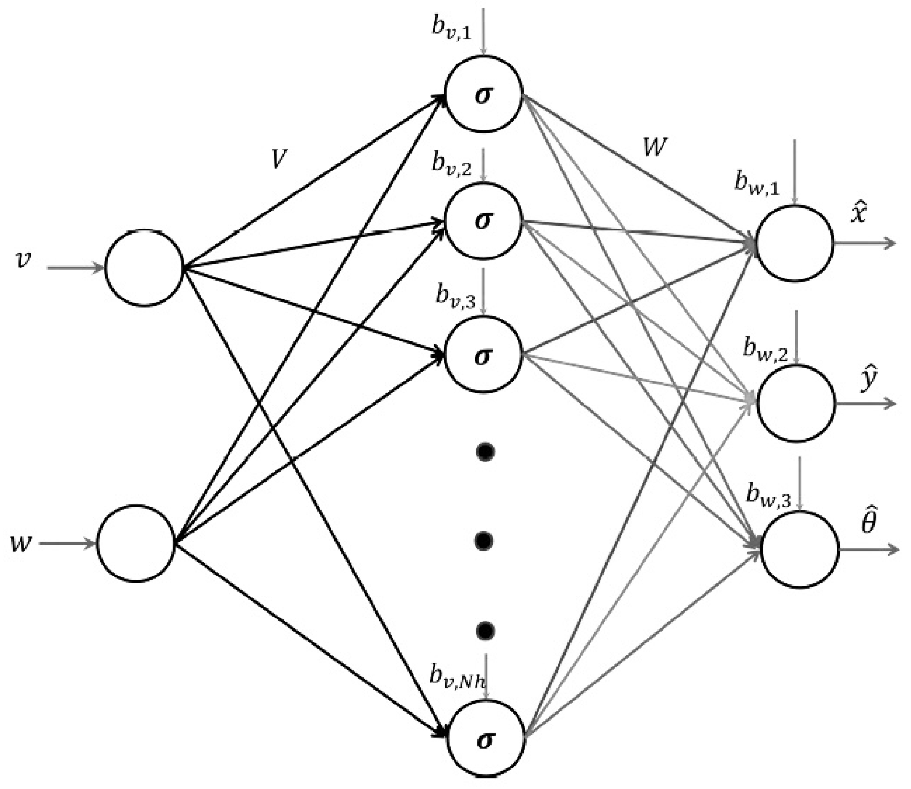
3.3. Jacobian Calculation Using the NN Model

The neural network (NN) serves the purpose of recognizing and approximating the robot system. Illustrated in Figure 3, the NN identification topology comprises a single hidden layer, an input layer with two inputs and an output layer with three outputs. The neural network’s inputs, denoted as $u=[v;w]$, correspond to the linear and angular velocity components, while its output is the predicted state of the mobile robot. The determination of the NN outputs is outlined as follows:

$$z_i=\sum _{j=1}^{Nh}\left(w_{i,j}{h}_j+b_{w,i}\right)$$

(18)

$$h_j=\sigma \left(\sum _{k=1}^{Ni}{v}_{j,k}{u}_k+b_{v,j}\right)$$

(19)

where $z=\hat{q}={\left[\begin{array}{ccc}\hat{x}& \hat{y}& \hat{\theta }\end{array}\right]}^T$ is the output of the NN, $h_j$ is the output of the hidden layer of the neural network, and $\sigma$ is the activation function.

The Jacobian matrix can be calculated from the NN identification formulas of Equations (18) and (19) by performing the following derivations:

$$\begin{array}{c}\hat{J}=\frac{\partial z}{\partial u}=\frac{\partial \hat{q}}{\partial u}=\left(\begin{array}{cc}\frac{\partial \hat{x}}{\partial v}& \frac{\partial \hat{x}}{\partial w}\\ \frac{\partial \hat{y}}{\partial v}& \frac{\partial \hat{y}}{\partial w}\\ \frac{\partial \hat{\theta }}{\partial v}& \frac{\partial \hat{\theta }}{\partial w}\end{array}\right)\hfill \end{array}$$

(20)

Applying the chain rule [47], the derivative for computing the Jacobian matrix is expressed as follows:

$$\frac{\partial z}{\partial u}=\frac{\partial z}{\partial h}\frac{\partial h}{\partial u}$$

(21)

where the derivatives of Equation (21) previous can be calculated as follows:

$$\frac{\partial z_i}{\partial h_j}=w_{i,j}\sum _{j=1}^{Nh}\left(w_{i,j}{h}_j\right)$$

(22)

$$\frac{\partial h_j}{\partial u_k}=v_{j,k}\sigma \left(\sum _{k=1}^{Ni}{v}_{j,k}{u}_k\right)$$

(23)

Therefore, using Equations (22) and (23), Equation (21) is given as follows:

$$\frac{\partial z_i}{\partial u_k}=\frac{\partial z_i}{\partial h_j}\frac{\partial h_j}{\partial u_k}=w_{i,j}\left(\sum _{j=1}^{Nh}\left(w_{i,j}{h}_j\right)\right)v_{j,k}\sigma \left(\sum _{k=1}^{Ni}{v}_{j,k}{u}_k\right)$$

(24)

Online updating of the Jacobian matrix estimation is employed to dynamically adjust the gains of the PID controller. Simultaneously, the NN weights undergo online tuning through a backpropagation algorithm (BPA) as described in [48]. This iterative tuning enhances the accuracy of the system’s Jacobian approximation, consequently improving the performance of the tracking control.

3.4. Discrete Extended Kalman Filter for NN Adaptation

The discrete extended Kalman filter (DEKF) is widely recognized as an algorithm for NN parameter estimation, as evidenced in prior studies [49]. Its appeal is attributed to its ease of implementation and computationally efficient calculations, which are particularly beneficial for nonlinear systems and practical applications [50]. For adaptive NN control based on DEKF, the weights of the NN are considered as the states that Kalman filter attempts to estimate, and the outputs of the NN are the optimal control signals of the WMR, as shown in Figure 2. The discrete nonlinear system for the NN adaptation process is given as follows [50]:

$${\theta }_k=f\left({\theta }_{k-1}\right)$$

(25)

$$z_k=h\left({\theta }_k,x_k\right)+v_k$$

(26)

where ${\theta }_k$ denotes the state vector encompassing all the NN weight parameters. The output of the NN is represented by $z_k$, while $v_k$ denotes an unknown bounded error. The input vector of the NN is denoted as $x_k$, and $h\left(\right)$ signifies the function of the NN. The algorithm for adapting the NN using the Kalman filter can be succinctly summarized as follows:

• State estimate propagation:

  $${\hat{\theta }}_{k|k-1}=f\left({\hat{\theta }}_{k-1|k-1}\right)$$

  (27)

  $$P_{k|k-1}=A_k{P}_{k-1|k-1}{A_k}^T+Q_{k-1}$$

  (28)
• The updated equations of the Kalman filter (or correction) are given as follows:

  $$K_k=P_{k|k-1}{H_k}^T{\left(H_k{P}_{k|k-1}{H_k}^T+R\right)}^{-1}$$

  (29)

  $${\hat{\theta }}_{k|k}={\hat{\theta }}_{k|k-1}+K_k\left(d_k-h\left({\hat{\theta }}_{k|k-1},0\right)\right)$$

  (30)

  $$P_{k|k}=\left(I-K_k{H}_k\right)P_{k|k-1}$$

  (31)

where $d_k$ in Equation (30) represents the reference or the desired control signal. Many variables affect the DEKF learning algorithm’s performance. These variables are matrices that must be correctly initialized; otherwise, the DEKF algorithm can exhibit poor learning performance and can exhibit negative impacts on the stability of the system. These matrices are the covariance matrix P, the covariance matrix learning rate R and the additional process noise matrix Q.

3.4.1. Stochastic Stability Analysis

Consider a nonlinear control system represented as follows:

$${\theta }_{k+1}=f\left({\theta }_k\right)$$

(32)

$$z_k=h\left({\theta }_k,x_k\right)+v_k$$

(33)

where ${\theta }_k\in R^n$ denotes the state of the system, $z_k$ represents the output of the system, $v_k$ is unknown noise, and $x_k$ are the inputs of the NN; f and h are continuously differentiable at ${\hat{\theta }}_{k|k}$ and ${\hat{\theta }}_{k|k-1}$, respectively. Developing Equations (32) and (33) using Taylor expansion gives [51]:

$$f\left({\theta }_k\right)-f\left({\hat{\theta }}_{k|k}\right)=A_k\left({\theta }_k-{\hat{\theta }}_{k|k}\right)+\varphi ({\theta }_k,{\hat{\theta }}_{k|k})$$

(34)

$$h\left({\theta }_k,x_k\right)-h\left({\hat{\theta }}_{k|k-1},x_k\right)=H_k\left({\theta }_k-{\hat{\theta }}_{k|k-1},x_k\right)+\chi ({\theta }_k,{\hat{\theta }}_{k|k},x_k)$$

(35)

where $\varphi$ and $\chi$ denote the residue terms. Therefore, the estimation errors are defined as follows:

$$e_{k+1|k}={\theta }_{k+1}-{\hat{\theta }}_{k+1|k}$$

(36)

$$e_{k+1|k+1}={\theta }_{k+1}-{\hat{\theta }}_{k+1|k+1}$$

(37)

According to Equations (36) and (37), the derivative can be calculated as follows:

$$\begin{array}{c}{e}_{k+1|k+1}=f\left({\theta }_k\right)-f\left({\hat{\theta }}_{k|k}\right)-k_k\left(h\left({\theta }_{k+1}\right)-h\left({\hat{\theta }}_{k+1|k}\right)\right)\hfill \\ ={\mathrm{A}}_k({\theta }_k-{\hat{\theta }}_{k|k})+\varphi ({\theta }_k,{\hat{\theta }}_{k|k})-K_k{H}_k({\theta }_{k+1}-{\hat{\theta }}_{k+1|k})-K_k\chi ({\theta }_{k+1},{\hat{\theta }}_{k+1|k})\hfill \\ =\left(I-k_k{H}_k\right)e_{k+1|k}+\varphi ({\theta }_k,{\hat{\theta }}_{k|k})-K_k\chi ({\theta }_{k+1},{\hat{\theta }}_{k+1|k})\hfill \end{array}$$

(38)

$$e_{k+1|k}={\mathrm{A}}_k\left(I-K_k{H}_k\right)e_{k|k-1}+r_k+s_k$$

(39)

where

$$r_k=\varphi ({\theta }_k,{\hat{\theta }}_{k|k})-K_k\chi ({\theta }_{k+1},{\hat{\theta }}_{k+1|k})$$

(40)

$$s_k=-K_v{v}_k$$

(41)

Definition 1.

The estimation error $e_{k|k}$ is exponentially bounded if there are real numbers $\overline{\eta },v>0$ and $0<\gamma <1$ such that:

$$E\left[{∥e_{k|k}∥}^2\right]\le \overline{\eta }{∥e_{0|0}∥}^2\gamma +v$$

(42)

In addition, the stochastic process is bounded if $sup∥e_{k|k}∥<\infty ,k\ge 0$.

3.4.2. Boundedness of the Estimation Error

This section demonstrates that the estimation error produced by the extended Kalman filter remains bounded if the following assumption holds:

Assumption 1.

There are real constants $\overline{a},\overline{h},\overline{p},\underline{p},\underline{q},\underline{r}>0$ such that:

$$\begin{array}{c}∥A_k∥\le \overline{a},∥H_k∥\le \overline{c},\underline{\mathrm{p}}{\mathrm{I}}_n\le P_k\le \overline{\mathrm{p}}{\mathrm{I}}_n\hfill \\ \underline{\mathrm{q}}{\mathrm{I}}_n\le Q_k,\overline{\mathrm{r}}{\mathrm{I}}_n\le R_k\hfill \end{array}$$

(43)

Assumption 2.

The nonlinear functions φ and χ are bounded if there are real numbers ${ϵ}_{\phi },{ϵ}_{\chi },{\kappa }_{\phi },{\kappa }_{\chi }\ge 0$ such that:

$$∥\varphi ({\theta }_k,{\hat{\theta }}_{k|k})∥\le {\kappa }_{\phi }{∥{\theta }_k-{\hat{\theta }}_{k|k}∥}^2$$

(44)

$$∥\chi ({\theta }_{k+1},{\hat{\theta }}_{k+1|k})∥\le {\kappa }_{\chi }{∥{\theta }_{k+1}-{\hat{\theta }}_{k+1|k}∥}^2$$

(45)

for $∥{\theta }_k-{\hat{\theta }}_{k|k}∥\le {ϵ}_{\phi }$ and $∥{\theta }_{k+1}-{\hat{\theta }}_{k+1|k}∥\le {ϵ}_{\chi }$

Lemma 1.

Suppose there is stochastic process $V_k\left(e_{k|k-1}\right)$ and positive real numbers $\overline{v},\underline{v},\mu >0$ and $0<\beta \le 1$ such that:

$$\overline{v}{∥V_k\left(e_{k|k-1}\right)∥}^2\le V_k\left(e_{k|k-1}\right)\le \underline{v}{∥V_k\left(e_{k|k-1}\right)∥}^2$$

(46)

$$E\left[V_{k+1}\left(e_{k+1|k}\right)\right]-V_k\left(e_{k|k-1}\right)\le -\beta V_k\left(e_{k|k-1}\right)+\mu$$

(47)

Equations (46) and (47) guarantee the boundedness of the estimation error.

Lemma 2.

Under Assumption 1, assume there is a real positive number $0<\alpha <1$ and ${\Pi }_k={P_k}^{-1}$ that satisfies the inequality:

$${\left(A_k\left(I-K_k{H}_k\right)\right)}^T{\Pi }_{k+1}\left(A_k\left(I-K_k{H}_k\right)\right)\le (1-\alpha ){\Pi }_k$$

(48)

where $1-\alpha =1/\left(1+\frac{\underline{q}}{\overline{p}{\left(\overline{a}+\overline{a}\overline{p}{\overline{c}}^2/\phantom{\overline{a}\overline{p}{\overline{c}}^2\underline{r}}\underline{r}\right)}^2}\right)$

Lemma 3.

Under Assumption 2, by defining ${\Pi }_k={P_k}^{-1}$, there are real numbers $\overline{ϵ},{\kappa }_{max}>0$ such that:

$${r_k}^T{\Pi }_k\left[2\left(A_k-K_k{H}_k\right)\left({\theta }_k-{\hat{\theta }}_{k|k}\right)+r_k\right]\le {\kappa }_{max}{∥{\theta }_k-{\hat{\theta }}_{k|k}∥}^3$$

(49)

holds for $∥{\theta }_k-{\hat{\theta }}_{k|k}∥\le \overline{ϵ}$, where $\overline{ϵ}=min\left({ϵ}_{\phi },{ϵ}_{\chi }\right)$.

Lemma 4.

Let Assumption 1 hold, and let ${\Pi }_k={P_k}^{-1}$ and $K_k,s_k$ be defined as in (41); therefore, there are positive real numbers ${\kappa }_{noise},\delta >0$ such that:

$$E\left[s_k{\Pi }_{k+1}{s}_k\right]\le {\kappa }_{noise}\delta$$

(50)

Theorem 1.

Consider the nonlinear stochastic system given by (32) and (33). Let Assumption 1 hold. Then the estimation error $V_k\left(e_{k|k}\right)$ is exponentially bounded by the mean square provided that the initial estimation error satisfies:

$$∥V_0\left(e_{0|0}\right)∥\le ϵ$$

(51)

where $ϵ>0$.

Proof. 

By choosing

$$V_k\left(e_{k|k-1}\right)={e_{k|k-1}}^T{\Pi }_k{e}_{k|k-1},$$

(52)

with ${\Pi }_k={P_k}^{-1}$, therefore

$$\overline{v}{∥V_k\left(e_{k|k-1}\right)∥}^2\le V_k\left(e_{k|k-1}\right)\le \underline{v}{∥V_k\left(e_{k|k-1}\right)∥}^2$$

(53)

where $\overline{v}=\frac{1}{\overline{p}}$ and $\underline{v}=\frac{1}{\underline{p}}$. □

To satisfy the requirements for the application of Lemma 2, an upper bound is needed on $E\left[V_{k+1}\left(e_{k+1|k}\right)\right]$. From Equation (39), the upper bound becomes as follows:

$$\begin{array}{c}{V}_{k+1}\left(e_{k+1|k}\right)={e_{k+1|k}}^T{\Pi }_{k+1}{e}_{k+1|k}\hfill \\ ={\left[{\mathrm{A}}_k\left(I-K_k{H}_k\right)e_{k|k-1}+r_k+s_k\right]}^T{\Pi }_{k+1}\left[{\mathrm{A}}_k\left(I-K_k{H}_k\right)e_{k|k-1}+r_k+s_k\right]\hfill \\ ={\left({\mathrm{A}}_k\left(I-K_k{H}_k\right)e_{k|k-1}\right)}^T{\Pi }_{k+1}\left({\mathrm{A}}_k\left(I-K_k{H}_k\right)e_{k|k-1}\right)\hfill \\ +{\left({\mathrm{A}}_k\left(I-K_k{H}_k\right)e_{k|k-1}\right)}^T{\Pi }_{k+1}\left(r_k+s_k\right)\hfill \\ +{\left(r_k+s_k\right)}^T{\Pi }_{k+1}\left({\mathrm{A}}_k\left(I-K_k{H}_k\right)e_{k|k-1}\right)+{\left(r_k+s_k\right)}^T{\Pi }_{k+1}\left(r_k+s_k\right)\hfill \\ ={e_{k|k-1}}^T{\left({\mathrm{A}}_k\left(I-K_k{H}_k\right)\right)}^T{\Pi }_{k+1}\left({\mathrm{A}}_k\left(I-K_k{H}_k\right)\right)e_{k|k-1}\hfill \\ +{\left(r_k+s_k\right)}^T{\Pi }_{k+1}\left[2{\mathrm{A}}_k\left(I-K_k{H}_k\right)e_{k|k-1}+r_k+s_k\right]\hfill \\ +2{s_k}^T{\Pi }_{k+1}\left[{\mathrm{A}}_k\left(I-K_k{H}_k\right)e_{k|k-1}+r_k+s_k\right]+{s_k}^T{\Pi }_{k+1}{s}_k\hfill \end{array}$$

(54)

Applying Lemma 1 in (52), the equation becomes as follows:

$$\begin{array}{c}{V}_{k+1}\left(e_{k+1|k}\right)=(1-\alpha )V_k\left(e_{k|k-1}\right)+{\left(r_k+s_k\right)}^T{\Pi }_{k+1}\left[2{\mathrm{A}}_k\left(I-K_k{H}_k\right)e_{k|k-1}+r_k+s_k\right]\hfill \\ +2{s_k}^T{\Pi }_{k+1}\left[{\mathrm{A}}_k\left(I-K_k{H}_k\right)e_{k|k-1}+r_k+s_k\right]+{s_k}^T{\Pi }_{k+1}{s}_k\hfill \end{array}$$

(55)

Taking the conditional expectation $E\left[V_{k+1}\left(e_{k+1|k}\right)\right]$ and considering the white noise property, the remaining terms are estimated via Lemmas 2 and 3, yielding:

$$E\left[V_{k+1}\left(e_{k+1|k}\right)\right]-V_k\left(e_{k|k-1}\right)\le -\alpha V_k\left(e_{k|k-1}\right)+{\kappa }_{max}{∥e_{k|k-1}∥}^3+{\kappa }_{noise}\delta$$

(56)

for $∥e_{k|k-1}∥\le {ϵ}^{\prime }$ defining:

$$ϵ=min\left({ϵ}^{\prime },\frac{\alpha }{2\overline{p}{\kappa }_{max}}\right)$$

(57)

with (52) and (52) for $∥e_{k|k-1}∥\le ϵ$

$${\kappa }_{max}∥e_{k|k-1}∥{∥e_{k|k-1}∥}^2\le \frac{\alpha }{2\overline{p}}{∥e_{k|k-1}∥}^2\le \frac{\alpha }{2}{V}_k\left(e_{k|k-1}\right)$$

(58)

Inserting into (57) yields:

$$E\left[V_{k+1}\left(e_{k+1|k}\right)\right]-V_k\left(e_{k|k-1}\right)\le -\frac{\alpha }{2}{V}_k\left(e_{k|k-1}\right)+{\kappa }_{noise}\delta$$

(59)

for $∥e_{k|k-1}∥\le ϵ$. Therefore, by applying Lemma 2 with $∥e_{0|0}∥\le ϵ$, $\underline{v}=\frac{1}{\overline{p}}$ and $\mu ={\kappa }_{noise}\delta$. However, by taking care that for $\widetilde{ϵ}\le ∥e_{k|k-1}∥\le ϵ$ with some $\widetilde{ϵ}\le ϵ$, the supermartingale inequality is as follows:

$$E\left[V_{k+1}\left(e_{k+1|k}\right)\right]-V_k\left(e_{k|k-1}\right)\le -\frac{\alpha }{2}{V}_k\left(e_{k|k-1}\right)+{\kappa }_{noise}\delta \le 0$$

(60)

To guarantee the boundedness of the estimation error, we choose:

$$\delta =\frac{\alpha }{2\overline{p}{\kappa }_{noise}}{\widetilde{ϵ}}^2$$

(61)

with $\widetilde{ϵ}$; therefore, for $∥e_{k|k-1}∥\ge \widetilde{ϵ}$

$${\kappa }_{noise}\delta \le \frac{\alpha }{2\overline{p}}{∥e_{k|k-1}∥}^2\le \frac{\alpha }{2}{V}_k\left(e_{k|k-1}\right)$$

(62)

It is concluded that the estimation error is bounded if the initial error and the noise terms are verified and bounded by (51) and (43). In this section, it is demonstrated that the estimation error produced by the extended Kalman filter remains bounded if the initial error and the noise terms are bounded.

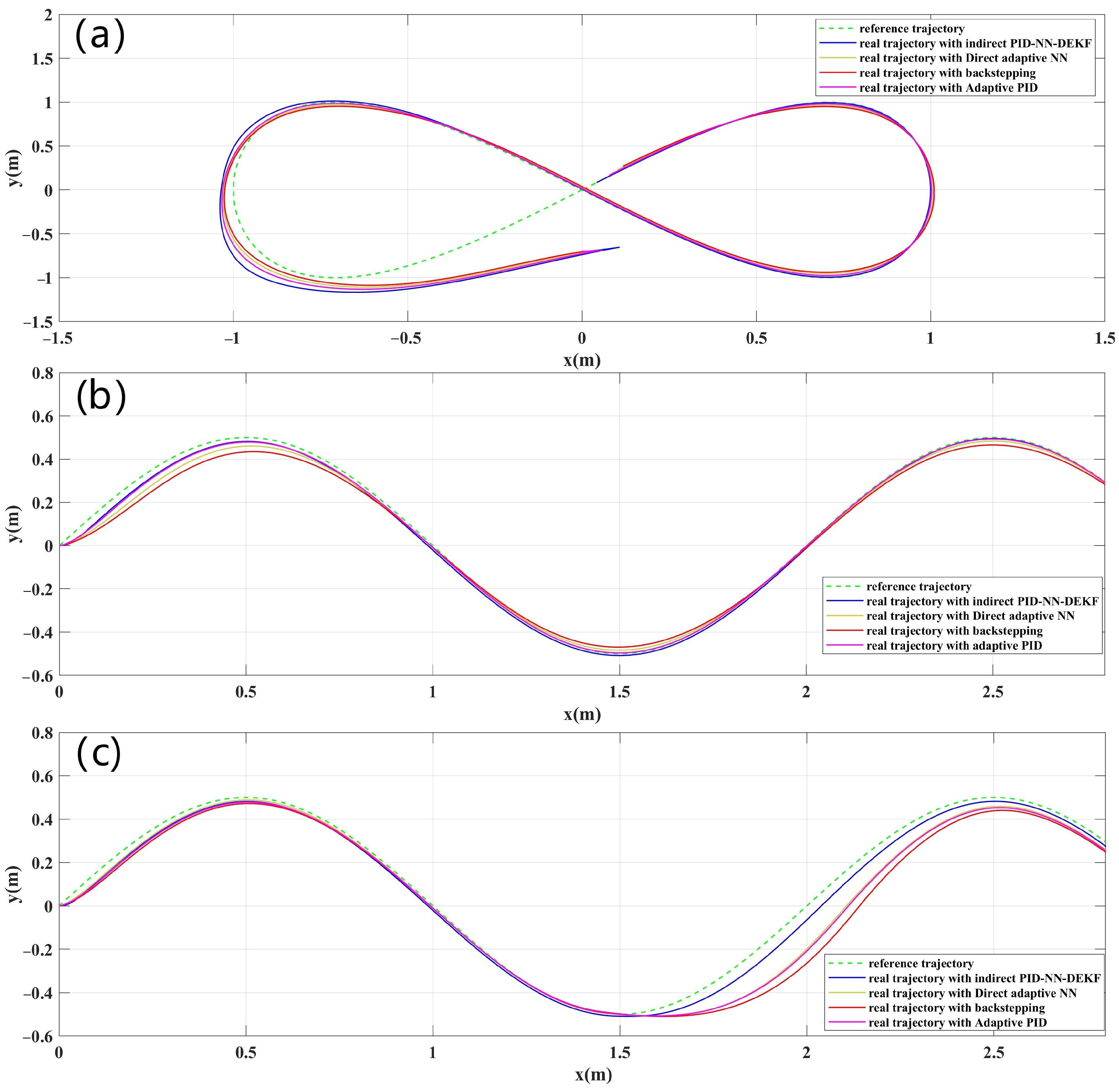
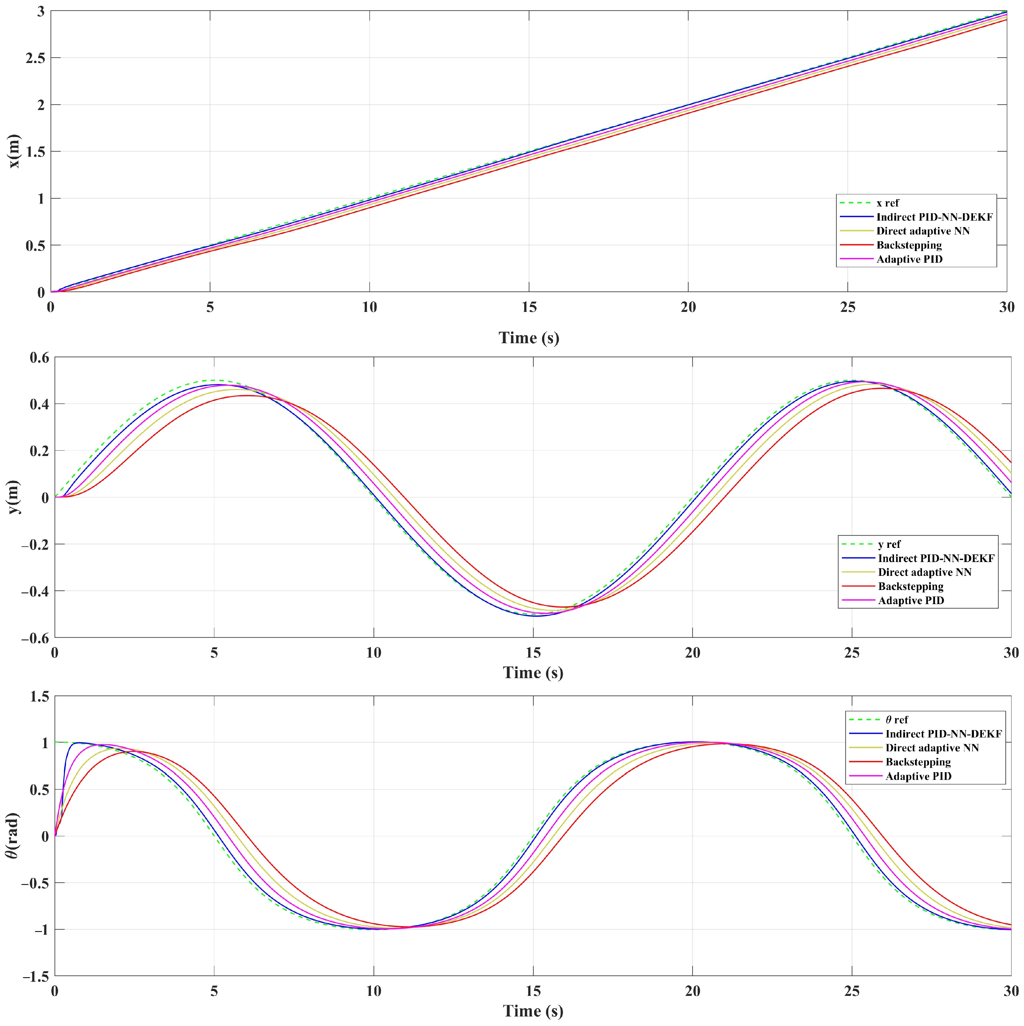
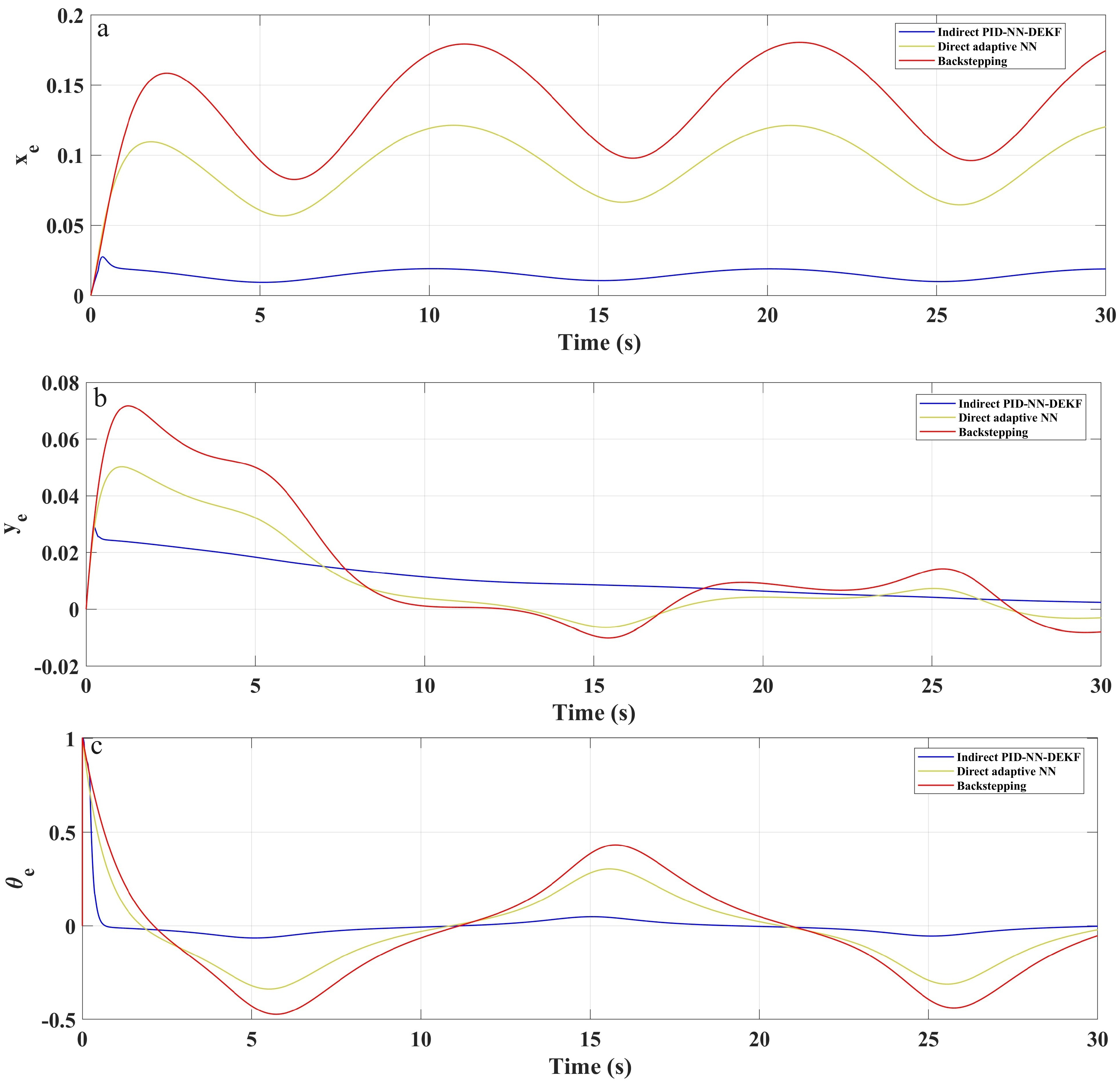
4. Results and Discussion

The primary objective of this research is to demonstrate the effectiveness of the proposed IAPID-NN-DEKF control strategy for tracking the trajectory of a WMR. This study is based on the implementation of adaptive control schemes, which are represented in the IAPID-NN-DEKF as NN adaptation and state estimation and are compared to DA-NN, BSC and the adaptive PID control techniques. The proposed schemes are tested, analyzed and compared under the same operating conditions, the same reference trajectory and the same initial robot posture to prove their effectiveness for WMR trajectory tracking. The learning rates are set to ${\mu }_{p,i,d}=0.9$ for linear and angular velocities. Hence, the parameters for DEKF for the IAPID-NN-DEKF are chosen as follows:

$$\begin{array}{c}{P}_0=I_{ns,ns}\times 1000\hfill \\ Q=I_{ns,ns}\times {10}^{-5}\hfill \\ R=\left[\begin{array}{ccc}1000& 0& 0\\ 0& 1000& 0\\ 0& 0& 1000\end{array}\right]\hfill \end{array}$$

(63)

Evaluation of the root mean square error (RMSE) is undertaken as a performance criterion, with the RMSE calculated according to the following equation:

$$RMSE=\sqrt{\frac{1}{n}\sum _{i=1}^n{\left(X\left(i\right)-X_r\left(i\right)\right)}^2}$$

(64)

where $X\left(i\right)$, $X_r\left(i\right)$ are vectors representing the actual and reference values at the i-th data point, respectively, and n denotes the total number of data points.

Figure 4 shows the lemniscate and the sinusoidal reference paths with the real tracked paths of the WMR using the proposed controllers. The inherent complexity of the lemniscate trajectory provides a challenging test for the control system: assessing its ability to navigate intricate paths and adapt to dynamic changes. By incorporating continuous variations in curvature, the lemniscate demands the control system to handle maneuvers with different turning radii: offering insights into its versatility. This choice is motivated by a desire to evaluate the robustness of the control system, as the lemniscate shape introduces complexities that simulate real-world uncertainties and disturbances. Moreover, using a lemniscate reflects a commitment to realism, as trajectories in practical scenarios rarely conform to perfect circles or straight lines. Benchmarking the performance of the control system against the lemniscate allows for a quantitative assessment, with metrics like root mean square error (RMSE) providing a measure of how closely the WMR follows the desired trajectory. Ultimately, the lemniscate serves as a comprehensive and challenging reference path that aids with assessing the adaptability, robustness and real-world applicability of the proposed control strategies. The dashed green line represents the reference trajectory; hence, the solid blue, yellowish, red and pink lines represent the trajectories followed by the mobile robot for the proposed schemes. According to this figure, it can be noted that the IAPID-IN-DEIF controller has more precise tracking performance compared to DA-NN, BSC and the adaptive PID, even when applying perturbation from $t=15$ s to $t=20$ s. The IAPID-NN-DEKF tracking performance confirms the effectiveness of the adaptive control scheme: using adaptive NN-DEKF and the good performance of DEKF for NN weight adaptation. Further, the RMSE indexes in

Table 1. Root mean squared error (RMSE) for different control strategies (lemniscate).

Control Strategy	RMSE of x	RMSE of y	RMSE of $\mathit{\theta }$
Indirect PID-NN-DEKF	0.078769	0.12086	0.1672
Backstepping	0.1139	0.2066	0.3409
Adaptive NN	0.1041	0.1832	0.2973
Adaptive PID	0.0917	0.1523	0.2375

,

Table 2. Root mean squared error (RMSE) for different control strategies (sinusoidal).

Control Strategy	RMSE of x	RMSE of y	RMSE of $\mathit{\theta }$
Indirect PID-NN-DEKF	0.01233	0.015138	0.088707
Backstepping	0.0475	0.0563	0.1586
Adaptive NN	0.0319	0.0380	0.1134
Adaptive PID	0.0384	0.0453	0.1326

and

Table 3. Root mean squared error (RMSE) for different control strategies (sinusoidal with perturbation).

Control Strategy	RMSE of x	RMSE of y	RMSE of $\mathit{\theta }$
Indirect PID-NN-DEKF	0.021495	0.016504	0.090142
Backstepping	0.0908	0.1076	0.1794
Adaptive NN	0.0617	0.0739	0.12512
Adaptive PID	0.0583	0.0415	0.1252

show that the tracking performance of the mobile robot is slightly improved when using IAPID-NN-DEKF instead of conventional DA-NN, BSC and the adaptive PID control techniques over the three proposed trajectories. Further, it is clearly noted from this table that IAPID-NN-DEKF shows highly reduced trajectory error and has a smaller RMSE compared to the other schemes. This note shows the high superiority of the IAPID-NN-DEKF structure for mobile robot trajectory tracking.

In Figure 5, Figure 6 and Figure 7, the mobile robot’s position coordinates ($x,y$ and $\theta$) are depicted as the reference coordinates for the lemniscate trajectory. In addition, Figure 8, Figure 9 and Figure 10 illustrate the tracking errors for $x_e,y_e$ and ${\theta }_e$ for different trajectories. Analysis of these figures reveals the efficacy of the implemented control scheme: IAPID-NN-DEKF achieved stable speed and high accuracy during mobile robot trajectory tracking.

5. Conclusions

This research paper introduced and evaluated an adaptive control scheme, IAPID-NN-DEKF, for addressing the challenges associated with the trajectory tracking and state estimation of wheeled mobile robots (WMRs). The proposed scheme leverages an adaptive indirect control proportional-integral-derivative (PID) controller using a neural network (NN) and discrete extended Kalman filter (DEKF).

The simulation results demonstrate the efficacy of the IAPID-NN-DEKF controller for achieving precise trajectory tracking. A lemniscate reference path was followed with superior accuracy; the controller outperformed the conventional DA-NN, backstepping (BSC) and adaptive PID control techniques. IAPID-NN-DEKF exhibited a more stable and accurate trajectory, as evidenced by the tracking errors depicted in the results.

Quantitative analysis further supports the superior performance of the IAPID-NN-DEKF scheme. The root mean squared error (RMSE) values for different control strategies indicate a noticeable reduction in trajectory tracking error: emphasizing the enhanced accuracy achieved by the proposed controller. IAPID-NN-DEKF outperforms DA-NN, BSC and the adaptive PID control strategies in terms of RMSE, showcasing its effectiveness at achieving accurate control and state estimation. In conclusion, the IAPID-NN-DEKF scheme demonstrates a high level of superiority for mobile robot trajectory tracking. The integration of adaptive control through an NN and DEKF contributes to the scheme’s adaptability to dynamic environments, computational efficiency and improved accuracy in state estimation. This research significantly advances the field of robust control techniques for WMRs and provides valuable insights into the potential of the proposed IAPID-NN-DEKF approach for real-world applications.

References

1. Shafaei, S.M.; Mousazadeh, H. Development of a mobile robot for safe mechanical evacuation of hazardous bulk materials in industrial confined spaces. J. Field Robot. 2022, 39, 218–231. [Google Scholar] [CrossRef]
2. Luo, F.; Zhou, Q.; Fuentes, J.; Ding, W.; Gu, C. A Soar-Based Space Exploration Algorithm for Mobile Robots. Entropy 2022, 24, 426. [Google Scholar] [CrossRef]
3. Kot, T.; Novák, P. Application of virtual reality in teleoperation of the military mobile robotic system TAROS. Int. J. Adv. Robot. Syst. 2022, 15, 1729881417751545. [Google Scholar] [CrossRef]
4. Bhondve, T.B.; Satyanarayan, R.; Mukhedkar, M. Mobile rescue robot for human body detection in rescue operation of disaster. Int. J. Adv. Res. Electr. Electron. Instrum. Eng. 2014, 3, 9876–9882. [Google Scholar]
5. West, A.; Tsitsimpelis, I.; Licata, M.; Jazbec, A.; Snoj, L.; Joyce, M.J.; Lennox, B. Use of Gaussian process regression for radiation mapping of a nuclear reactor with a mobile robot. Sci. Rep. 2021, 11, 13975. [Google Scholar] [CrossRef]
6. Matraji, I.; Al-Durra, A.; Haryono, A.; Al-Wahedi, K.; Abou-Khousa, M. Trajectory tracking control of skid-steered mobile robot based on adaptive second order sliding mode control. Control Eng. Pract. 2018, 72, 167–176. [Google Scholar] [CrossRef]
7. Saradagi, A.; Muralidharan, V.; Krishnan, V.; Menta, S.; Mahindrakar, A.D. Formation control and trajectory tracking of nonholonomic mobile robots. IEEE Trans. Control Syst. Technol. 2017, 26, 2250–2258. [Google Scholar] [CrossRef]
8. Hao, Y.; Wang, J.; Chepinskiy, S.A.; Krasnov, A.J.; Liu, S. Backstepping based trajectory tracking control for a four-wheel mobile robot with differential-drive steering. In Proceedings of the 2017 36th Chinese Control Conference (CCC), Dalian, China, 26–28 July 2017; pp. 4918–4923. [Google Scholar]
9. Rubagotti, M.; Della Vedova, M.L.; Ferrara, A. Time-optimal sliding-mode control of a mobile robot in a dynamic environment. IET Control Theory Appl. 2011, 5, 1916–1924. [Google Scholar] [CrossRef]
10. Bencherif, A.; Chouireb, F. A recurrent TSK interval type-2 fuzzy neural networks control with online structure and parameter learning for mobile robot trajectory tracking. Appl. Intell. 2019, 49, 3881–3893. [Google Scholar] [CrossRef]
11. Talaat, F.M.; Ibrahim, A.; El-Kenawy, E.S.M.; Abdelhamid, A.A.; Alhussan, A.A.; Khafaga, D.S.; Salem, D.A. Route Planning for Autonomous Mobile Robots Using a Reinforcement Learning Algorithm. Actuators 2022, 12, 12. [Google Scholar] [CrossRef]
12. Zhao, W.; Gu, L. Adaptive PID Controller for Active Suspension Using Radial Basis Function Neural Networks. Actuators 2023, 12, 437. [Google Scholar] [CrossRef]
13. Sun, Y.; Liang, X.; Wan, Y.; Zhao, W.; Gu, L. Tracking Control of Robot Manipulator with Friction Compensation Using Time-Delay Control and an Adaptive Fuzzy Logic System. Actuators 2023, 12, 184. [Google Scholar] [CrossRef]
14. Zhao, P.; Chen, J.; Song, Y.; Tao, X.; Xu, T.; Mei, T. Design of a control system for an autonomous vehicle based on adaptive-pid. Int. J. Adv. Robot. Syst. 2012, 9, 44. [Google Scholar] [CrossRef]
15. Ouyang, P.R.; Acob, J.; Pano, V. PD with sliding mode control for trajectory tracking of robotic system. Robot. Comput.-Integr. Manuf. 2014, 30, 189–200. [Google Scholar] [CrossRef]
16. Liu, W.; Wang, X.; Liang, S. Trajectory tracking control for wheeled mobile robots based on a cascaded system control method. In Proceedings of the IECON 2020 the 46th Annual Conference of the IEEE Industrial Electronics Society, Singapore, 18–21 October 2020; pp. 396–401. [Google Scholar]
17. Wang, S.; Yin, X.; Li, P.; Zhang, M.; Wang, X. Trajectory tracking control for mobile robots using reinforcement learning and PID. Iran. J. Sci. Technol. Trans. Electr. Eng. 2020, 44, 1059–1068. [Google Scholar] [CrossRef]
18. Mok, R.; Ahmad, M.A. Fast and optimal tuning of fractional order PID controller for AVR system based on memorizable-smoothed functional algorithm. Eng. Sci. Technol. Int. J. 2022, 35, 101264. [Google Scholar] [CrossRef]
19. Kong, I.; Qian, I.; Wang, I. SPSA-based PID parameters optimization for a dual-tank liquid-level control system. In Proceedings of the 2016 IEEE International Conference on Industrial Engineering and Engineering Management (IEEM), Bali, Indonesia, 4–7 December 2016; pp. 1463–1467. [Google Scholar]
20. Wang, Z.; Zhang, J. Incremental PID Controller-Based Learning Rate Scheduler for Stochastic Gradient Descent. IEEE Trans. Neural Netw. Learn. Syst. 2022; Early Access. [Google Scholar] [CrossRef]
21. Cui, M.; Liu, W.; Liu, H.; Jiang, H.; Wang, Z. Extended state observer-based adaptive sliding mode control of differential-driving mobile robot with uncertainties. Nonlinear Dyn. 2016, 83, 667–683. [Google Scholar] [CrossRef]
22. Riccio, V.; Jahangirova, G.; Stocco, A.; Humbatova, N.; Weiss, M.; Tonella, P. Testing machine learning based systems: A systematic mapping. Empir. Softw. Eng. 2020, 25, 5193–5254. [Google Scholar] [CrossRef]
23. Hassan, N.; Saleem, A. Neural network-based adaptive controller for trajectory tracking of wheeled mobile robots. IEEE Access 2022, 10, 13582–13597. [Google Scholar] [CrossRef]
24. Liu, Z.; Peng, K.; Han, L.; Guan, S. Modeling and control of robotic manipulators based on artificial neural networks: A review. Iran. J. Sci. Technol. Trans. Mech. Eng. 2023, 47, 1307–1347. [Google Scholar] [CrossRef]
25. Nguyen, T.; Nguyentien, K.; Do T, P.T. Neural network-based adaptive sliding mode control method for tracking of a nonholonomic wheeled mobile robot with unknown wheel slips, model uncertainties, and unknown bounded external disturbances. Acta Polytech. Hung. 2018, 15, 103–123. [Google Scholar]
26. Abdelwahab, M.; Parque, V.; Elbab, A.M.F.; Abouelsoud, A.A.; Sugano, S. Trajectory tracking of wheeled mobile robots using z-number based fuzzy logic. IEEE Access 2020, 8, 18426–18441. [Google Scholar] [CrossRef]
27. Novák, V.; Lehmke, S. Logical structure of fuzzy IF-THEN rules. Fuzzy Sets Syst. 2006, 157, 2003–2029. [Google Scholar] [CrossRef]
28. Hsu, C.F.; Chen, B.R.; Lin, Z.L. Implementation and Control of a Wheeled Bipedal Robot Using a Fuzzy Logic Approach. Actuators 2022, 11, 357. [Google Scholar] [CrossRef]
29. Dorigo, M.; Birattari, M.; Stutzle, T. Ant colony optimization. IEEE Comput. Intell. Mag. 2006, 1, 28–39. [Google Scholar] [CrossRef]
30. Marini, F.; Walczak, B. Particle swarm optimization (PSO). A tutorial. Chemom. Intell. Lab. Syst. 2015, 149, 153–165. [Google Scholar] [CrossRef]
31. Silaa, M.Y.; Barambones, O.; Bencherif, A.; Rahmani, A. A New MPPT-Based Extended Grey Wolf Optimizer for Stand-Alone PV System: A Performance Evaluation versus Four Smart MPPT Techniques in Diverse Scenarios. Inventions 2023, 8, 142. [Google Scholar] [CrossRef]
32. Silaa, M.Y.; Barambones, O.; Cortajarena, J.A.; Alkorta, P.; Bencherif, A. PEMFC Current Control Using a Novel Compound Controller Enhanced by the Black Widow Algorithm: A Comprehensive Simulation Study. Sustainability 2023, 15, 13823. [Google Scholar] [CrossRef]
33. Yang, X.S.; He, X. Bat algorithm: Literature review and applications. J. Univ. Babylon Eng. Sci. 2013, 26, 292–306. [Google Scholar] [CrossRef]
34. Castillo, O.; Neyoy, H.; Soria, J.; Melin, P.; Valdez, F. A new approach for dynamic fuzzy logic parameter tuning in ant colony optimization and its application in fuzzy control of a mobile robot. Appl. Soft Comput. 2015, 128, 150–159. [Google Scholar] [CrossRef]
35. Saleh, A.L.; Hussain, M.A.; Klim, S.M. Optimal trajectory tracking control for a wheeled mobile robot using fractional order PID controller. Int. J. Bio-Inspired Comput. 2018, 5, 141–149. [Google Scholar] [CrossRef]
36. Morin, P.; Samson, C. Motion control of wheeled mobile robots. In Springer Handbook of Robotics; Springer: Berlin/Heidelberg, Germany, 2008; Volume 1, pp. 799–826. [Google Scholar]
37. Zhao, Y.; BeMent, S.L. Kinematics, dynamics and control of wheeled mobile robots. In Proceedings of the 1992 IEEE International Conference on Robotics and Automation, Nice, France, 12–14 May 1992; pp. 91–92. [Google Scholar]
38. Peng, Y.; Zhang, P.; Fang, Z.; Zheng, S.; Guo, Z. Trajectory tracking control of the wheeled mobile robot based on the curve tracking algorithm. J. Phys. Conf. Ser. 2023, 2419, 012106. [Google Scholar] [CrossRef]
39. Li, Z.; Deng, J.; Lu, R.; Xu, Y.; Bai, J.; Su, C.Y. Trajectory-tracking control of mobile robot systems incorporating neural-dynamic optimized model predictive approach. IEEE Trans. Syst. Man Cybern. Syst. 2015, 46, 740–749. [Google Scholar] [CrossRef]
40. Silaa, M.Y.; Barambones, O.; Bencherif, A. A Novel Adaptive PID Controller Design for a PEM Fuel Cell Using Stochastic Gradient Descent with Momentum Enhanced by Whale Optimizer. Electronics 2022, 11, 2610. [Google Scholar] [CrossRef]
41. Borase, R.P.; Maghade, D.K.; Sondkar, S.Y.; Pawar, S.N. A review of PID control, tuning methods and applications. Int. J. Dyn. Control 2021, 9, 818–827. [Google Scholar] [CrossRef]
42. He, N.; Yang, Z.; Fan, X.; Wu, J.; Sui, Y.; Zhang, Q. A Self-Adaptive Double Q-Backstepping Trajectory Tracking Control Approach Based on Reinforcement Learning for Mobile Robots. Actuators 2023, 12, 326. [Google Scholar] [CrossRef]
43. Yiğit, S.; Sezgin, A. Design of a Kinematic Model Based Backstepping PID and SMC for Mobile Robots. Sak. Univ. J. Sci. (SAUJS)/Sak. Üniv. Bilim. Enst. Derg. 2023, 27, 120. [Google Scholar]
44. Bengio, Y.; Goodfellow, I.; Courville, A. Deep learning. In Genetic Programming and Evolvable Machines; MIT Press: Cambridge, MA, USA, 2017; Volume 1. [Google Scholar]
45. Wu, H.; Zhang, X.; Song, L.; Zhang, Y.; Wang, C.; Zhao, X.; Gu, L. Parallel Network-Based Sliding Mode Tracking Control for Robotic Manipulators with Uncertain Dynamics. Actuators 2023, 12, 187. [Google Scholar] [CrossRef]
46. Chu, M.T.; Zhang, Z. An Innate Moving Frame on Parametric Surfaces: The Dynamics of Principal Singular Curves. Mathematics 2023, 11, 3306. [Google Scholar] [CrossRef]
47. Asadi, A.R.; Abbe, E. Chaining meets chain rule: Multilevel entropic regularization and training of neural networks. J. Mach. Learn. Res. 2020, 21, 5453–5484. [Google Scholar]
48. I. Breesam, W.; L. Saleh, A.; A. Mohamad, K.; J. Yaqoob, S.; A. Qasim, M.; T. Alwan, N.; Nayyar, A.; Al-Amri, J.F.; Abouhawwash, M. Speed control of a multi-motor system based on fuzzy neural model reference method. Actuators 2022, 11, 123. [Google Scholar] [CrossRef]
49. Kulikova, M.V.; Kulikov, G.Y. Data-driven parameter estimation in stochastic dynamic neural fields by state-space approach and continuous-discrete extended Kalman filtering. Digit. Signal Process. 2023, 136, 104010. [Google Scholar] [CrossRef]
50. Lv, C.; Lan, Z.; Chang, J.; Yu, D. Extended-Kalman-filter-based equilibrium manifold expansion observer for ramjet nonlinear control. Aerosp. Sci. Technol. 2023, 138, 108359. [Google Scholar] [CrossRef]
51. Linnainmaa, S. Taylor expansion of the accumulated rounding error. BIT Numer. Math. 1976, 16, 146–160. [Google Scholar] [CrossRef]
Figure 1. The mobile robot tracking error.
Actuators 13 00051 g001
Figure 2. Control scheme for indirect adaptive control based on NN.
Actuators 13 00051 g002
Figure 3. NN application for WMR identification in indirect adaptive control.
Actuators 13 00051 g003
Figure 4. Tracking response of the WMR for initial positions X 0 = [ 0 ; 0.7 ; π / 2 ] for the lemniscate and X 0 = [ 0 ; 0 ; 0 ] for the sinusoidal trajectories: (a) lemniscate, (b) sinusoidal, and (c) sinusoidal with perturbation.
Actuators 13 00051 g004
Figure 5. The position coordinates for lemniscate trajectory.
Actuators 13 00051 g005
Figure 6. The position coordinates for sinusoidal trajectory.
Actuators 13 00051 g006
Figure 7. The position coordinates for sinusoidal trajectory with perturbation.
Actuators 13 00051 g007
Figure 8. Tracking errors for (a) x e , (b) y e and (c) θ e for lemniscate trajectory.
Actuators 13 00051 g008
Figure 9. Tracking errors for x e , y e and θ e for sinusoidal trajectory.
Actuators 13 00051 g009
Figure 10. Tracking errors for x e , y e and θ e for sinusoidal trajectory with perturbation.
Actuators 13 00051 g010