Two-Stage Predefined-Time Exact Sliding Mode Control Based on Predefined-Time Exact Disturbance Observer

Abstract

This paper is concerned with the predefined-time exact sliding mode control issue of a class of high-order uncertain nonlinear systems with disturbances. The proposed control scheme is composed of a predefined-time exact disturbance observer and a two-stage predefined-time exact sliding mode controller. The disturbance observer can estimate the system disturbances accurately within an arbitrary predefined observation time, and the time can be set as the handover time between two control stages. The classic sliding mode controller guarantees bounded system states in the first control stage. Then, a predefined-time sliding mode controller is designed based on time-varying tuning function, regulating the system states to exact zero within a final predefined settling time in the second stage. It is shown that the control input signal is always chattering-free with respect to time. The effectiveness and superiority of the proposed control scheme is demonstrated with simulation examples.

1. Introduction

System settling time is a critical indicator to describe the performance and the efficiency of a controller. A Finite-time controller provides a finite upper bound of settling time (UBST) for a controlled system, but the UBST may vary with initial system conditions [1]. Then, a fixed-time controller guarantees a system to exhibit a uniform UBST which is independent on initial system conditions; however, the UBST may be formulated as a complex expression that contains a series of parameters [2]. Some complex calculations may be inevitable for UBST presetting when applying a fixed-time controller. Recently, predefined-time control (also named as prescribed-time control in some studies) has drawn much attention [3,4,5], since the provided UBST under a predefined-time controller is an explicit and direct parameter in the control algorithm. The parameter is uniform with respect to both initial system conditions and the other control parameters [6]. It is significantly convenient for users to know and adjust the UBST a priori via the exact parameter in a predefined-time control algorithm.

Designing predefined-time controllers with time-varying control gains is an effective approach that has been widely studied. Pal et al. [7] and Song et al. [8,9,10] proposed predefined-time controllers based on time-varying control gains that tend to infinity as the time tends to the predefined settling time. Singh et al. [11] proposed predefined-time controllers for large-scale systems using vector control Lyapunov functions and time-varying control gains. In order to avoid the problem that the time-varying gains may be unbounded as the time approaches to the predefined convergence time, Gómez-Gutiérrez [12,13] and Orlov [14] applied the time space deformation approach to switch the predefined-time controllers before the prescribed settling time. As for the control issue of nonlinear high-order strict-feedback systems, Fu et al. [15,16] and Ye and Song [17] proved that the predefined-time control input signal with infinite time-varying control gains can be guaranteed to be bounded if precise control is achieved.

Applying predefined-time stable Lypapunov dynamics is another available control approach for various nonlinear systems [18,19,20]. To overcome the potential singularity problem of the predefined-time control issue for high-order systems, Xie et al. [21] and Ding et al. [22] designed nonsingular predefined-time controllers for spacecraft and robot systems, ensuring that the attitude tracking errors converge into a small neighborhood of the origin within a predefined settling time. Xu et al. [23] and Zhang et al. [24] designed nonsingular adaptive predefined-time controllers for interconnected systems and stochastic systems by applying predefined-time stable Lypapunov dynamics with fractional powers. In addition, the time base generator (TBG) method [25,26] and the time-varying tuning function method [27,28,29] were investigated, transforming an original system to stable zero dynamics for predefined-time stabilization. Then, Lv et al. [30] took advantage of predefined-time stable Lypapunov dynamics and the time-varying tuning function method, proposing a nonsingular predefined-time backstepping controller for uncertain high-order systems and provided a less conservative UBST for presetting.

It is seen that if a system is affected by perturbations or disturbances, the asymptotic stability rather than the rigorous predefined-time stability of the controlled system is guaranteed under the TBG-based method [25,26]. In order to guarantee a controlled system with disturbances to exhibit rigorous predefined-time stability, the variable structure control strategy was widely utilized to deal with disturbances in the related studies [15,16,18,19,20,27,28,29]. It is known that the variable structure control algorithms with signum terms may lead to discontinuous control input signals. Such chattering control signals may deteriorate the components of a real physical system due to high-frequency oscillations, or may even be impossible to implement due to the limited actuator response [4]. In order to avoid the control input chattering issue under system disturbances, several continuous predefined-time controllers have been proposed, regulating the system error into a region with an arbitrary predefined bound within an arbitrary predefined UBST. For example, Cao et al. [31] designed a predefined-time and predefined-bound controller for nonlinear high-order strict-feedback systems with non-vanishing disturbances based on prescribed performance control method. Shao et al. [32] and Ye et al. [33] proposed predefined-time and predefined-bound controllers for uncertain second-order systems and spacecraft attitude systems using predefined-time stable Lypapunov dynamics. However, system errors at the predefined UBST may not be zero exactly under the continuous predefined-time algorithms [31,32,33], thus decreasing the control accuracy.

In order to enhance the practicality and the accuracy of a controller, this paper proposes a novel two-stage continuous predefined-time exact control scheme for a class of high-order uncertain nonlinear systems with disturbances based on time-varying tuning functions. We notice that traditional predefined-time controllers may lead to chattering control signal to handle system disturbances [15,16,18,19,20,27,28,29], and system steady errors may not be eliminated entirely at the final UBST under some continuous predefined-time control algorithms [31,32,33]. The aim of this paper is to overcome the problem of control signal chattering and to eliminate system errors at the predefined UBST simultaneously by designing a new two-stage predefined-time control scheme. A new predefined-time exact disturbance observer is constructed, estimating the system disturbances precisely within an arbitrary predefined observation time $t_d<t_s$. A two-stage high-order sliding mode controller is designed, regulating the system to equilibrium accurately within a final predefined settling time $t_s$. Predefined observation time $t_d$ and predefined settling time $t_s$ are two explicit parameters designed in two time-varying tuning functions involved in the structure of the observer and the controller, respectively. It is worth noting that the proposed control scheme has the following advantages compared with the previous predefined-time control studies:

(1) The control signal under the proposed controller is continuous and chattering-free when considering disturbances compared with [15,16,18,19,20,27,28,29]. There is no discontinuous term appearing in the direct expression of the proposed controller.

(2) The control accuracy after the predefined settling time is guaranteed rigorously. The proposed controller guarantees zero steady error at the provided UBST compared with [25,26,31,32,33], where the errors may not be eliminated essentially at the UBST.

(3) The control gains of the proposed controller are constant and bounded. The potential unbounded time-varying control gain is not involved compared with [7,8,9,10] when the time tends to the predefined settling time.

The reminder of the paper is organized as follows: Section 2 provides some preliminaries and formulates the problem studied in this paper. Section 3 presents the details of the predefined-time control scheme, which contains a predefined-time exact disturbance observer and a two-stage predefined-time exact sliding mode controller. Then, Section 4 demonstrates the effectiveness of the proposed control scheme with two simulation examples. Finally, Section 5 draws the conclusion of the paper.

Notation

In this paper, $\mathbb{R}$ is the set of real numbers, ${\mathbb{R}}_{\ne 0}$ is the set of non-zero real numbers. ${\mathbb{R}}^i$ is the set of an i-dimensional real vector, ${\mathbb{R}}^{i_1\times i_2}$ is the set of an $i_1\times i_2$ real matrix, $0_i\in {\mathbb{R}}^i$ is an i-dimensional zero vector and $I_i\in {\mathbb{R}}^{i\times i}$ is an $i\times i$ identity matrix. For any $y\in \mathbb{R}$, $\mathrm{sign}\left(y\right)$ is the signum function of y. For any vector $\eta \in {\mathbb{R}}^i$, ${\eta }^T$ is its transpose vector, and $\parallel \eta \parallel =\sqrt{{\eta }^T\eta }$. For any positive integer i, $i!=i\times (i-1)\times \dots \times 1$ is its factorial, with $0!=1$. For any nonnegative integer $i_1$ and $i_2$ with $i_1\ge i_2$, $A_{i_1}^{i_2}=i_1!/(i_1-i_2)!$ is the number of permutations.

2. Problem Formulation and Preliminaries

2.1. Preliminaries

Consider a non-autonomous nonlinear system:

$$\begin{array}{c}\hfill \dot{z}=G(t,z,T),z\left(t_0\right)=z_0\in {\mathbb{R}}^m\end{array}$$

(1)

where $z\in {\mathbb{R}}^m$ is the system state, $T\in (t_0,\infty )$ is a fixed system parameter with $t_0\in [0,\infty )$ being the initial control time, and $G:[t_0,\infty )\times {\mathbb{R}}^m\times (t_0,\infty )\to {\mathbb{R}}^m$ is piecewise continuous in t and globally Lipschitz in z. The solutions of (1) are given by $z(t,z_0,T)$. In the rest of the paper, the arguments of some functions are sometimes dropped if no confusion arises.

Definition 1. 

Ref. [29], The solutions of (1) are globally predefined-time stable if, for any $z_0\in {\mathbb{R}}^m$, $z(t,z_0,T)=0_m$ holds for all $t\in [T,\infty )$.

Notice that System (1) is equivalent to controlled system

$$\begin{array}{c}\hfill \dot{z}=H(t,z,v(t,z,T)),z\left(t_0\right)=z_0\in {\mathbb{R}}^m\end{array}$$

(2)

where $v:[t_0,\infty )\times {\mathbb{R}}^m\times (t_0,\infty )\to {\mathbb{R}}^p$ is a feedback control input, $H:[t_0,\infty )\times {\mathbb{R}}^m\times {\mathbb{R}}^p\to {\mathbb{R}}^m$, and $H(t,z,v)=G(t,z,T)$ holds for all $t\in [t_0,\infty )$. Now, if System (2) is globally predefined-time stable, one knows that the UBST of (2) can be known directly and set arbitrarily by users with explicit parameter T in input signal v.

Then, a lemma about the finite-time stability condition of a super-twisting system and another about the input-to-state stable (ISS) system are presented.

Lemma 1. 

Ref. [34], We consider system

$$\begin{array}{c}\hfill \left\{\begin{array}{c}{\dot{\lambda }}_1=-a_1{\left|{\lambda }_1\right|}^{\frac{1}{2}}\mathrm{sign}\left({\lambda }_1\right)+{\lambda }_2\hfill \\ {\dot{\lambda }}_2=-a_2\mathrm{sign}\left({\lambda }_1\right)+w\left(t\right)\hfill \end{array}\right.\end{array}$$

(3)

where ${\lambda }_1\in \mathbb{R}$ and ${\lambda }_2\in \mathbb{R}$ are system states, the system gains $a_1>0$ and $a_2>0$ are constant parameters, and $w\left(t\right)\le W$, with $W>0$ being a constant. Then, System (3) is finite-time stable if

$$\begin{array}{c}\hfill a_2>W,a_1>\sqrt{a_2+W}.\end{array}$$

(4)

Lemma 2. 

Ref. [35], We consider system

$$\dot{\chi }=F(t,\chi ,\nu )$$

(5)

where $\chi \in {\mathbb{R}}^m$ is the system state, $\nu \in {\mathbb{R}}^r$ is the system input, and $F:[t_0,\infty )\times {\mathbb{R}}^m\times {\mathbb{R}}^r\to {\mathbb{R}}^m$ is continuously differentiable and globally Lipschitz in $(\chi ,\nu )$, uniformly in t. If the unforced system $\dot{\chi }=F(t,\chi ,0)$ has a globally exponentially stable equilibrium point at origin $\chi =0_m$, then system (5) is ISS.

2.2. Problem Formulation of the Paper

We consider an uncertain nonlinear system [36]:

$$\begin{array}{c}\hfill \left\{\begin{array}{c}{\dot{x}}_i=x_{i+1},i=1,\dots ,n-1\hfill \\ {\dot{x}}_n=f(x,t)+b(x,t)u+d(x,t)\hfill \end{array}\right.\end{array}$$

(6)

with bounded initial system conditions $x_j\left(t_0\right)\in \mathbb{R}$$(j=1,\dots ,n)$, where $n\ge 2$ is the system order, $x={[x_1,\dots ,x_n]}^T\in {\mathbb{R}}^n$ is the system state vector, $f:{\mathbb{R}}^n\times [t_0,\infty )\to \mathbb{R}$ and $b:{\mathbb{R}}^n\times [t_0,\infty )\to {\mathbb{R}}_{\ne 0}$ are known continuous functions, $u\in \mathbb{R}$ is the control input signal, and $d:{\mathbb{R}}^n\times [t_0,\infty )\to \mathbb{R}$ represents the unknown system disturbances.

The objective of the paper is to design a disturbance observer,

$$\begin{array}{c}\hfill \dot{\xi }=g(t,t_d,x,u,\xi ),t\in [t_0,\infty )\end{array}$$

(7)

and a feedback control input signal,

$$\begin{array}{c}\hfill u=u(t,t_s,x,\xi ),t\in [t_0,\infty )\end{array}$$

(8)

such that

$$\begin{array}{cc}\hfill d(x,t)-{\xi }_2\left(t\right)=& 0,\mathrm{for}\mathrm{all}t\in [t_d,\infty )\hfill \end{array}$$

(9)

$$\begin{array}{cc}\hfill x\left(t\right)=& 0,\mathrm{for}\mathrm{all}t\in [t_s,\infty )\hfill \end{array}$$

(10)

where $t_s\in (t_0,\infty )$ is the predefined settling time of System (6), $t_d\in (t_0,t_s)$ is the predefined observation time of Disturbance observer (7), $\xi ={[{\xi }_1,{\xi }_2]}^T\in {\mathbb{R}}^2$ is the observer state vector, $g:[t_0,\infty )\times (t_0,t_s)\times {\mathbb{R}}^n\times \mathbb{R}\times {\mathbb{R}}^2\to {\mathbb{R}}^2$ is an update function, and u$:[t_0,\infty )\times (t_0,\infty )\times {\mathbb{R}}^n\times {\mathbb{R}}^2\to \mathbb{R}$ should be continuous with respect to time for all $t\in [t_0,\infty )$.

Remark 1. 

Predefined-time stabilization of System (6) is the eventual control objective. For any selected predefined settling time $t_s\in (t_0,\infty )$ of System (6), there exists time $t_d\in (t_0,t_s)$ being chosen as the predefined observation time of Disturbance observer (7). Thus, the predefined-time observation objective should be achieved before the predefined-time stabilization objective.

The following assumptions can be made without loss of generality.

Assumption 1. 

Ref. [36], The state vector $x\left(t\right)$ of System (6) is available for all $t\in [t_0,\infty )$.

Assumption 2. 

Ref. [36], The magnitude and rate of disturbance in System (6) is bounded, i.e., $\left|d(x,t)\right|\le l_0$ and $|\dot{d}(x,t)|\le l_1$ hold for all $t\in [t_0,\infty )$, where $l_0$ and $l_1$ are known positive constants.

Remark 2. 

Any single input and single output linear time-invariant system $\dot{\overline{x}}=A^{\ast }\overline{x}+B^{\ast }u$ can be transformed into an n-order Integrator system (6), provided it is controllable, by transforming the system into the so-called controllable canonical form and applying an input that cancels the open-loop dynamics of the nth state equation [25], where $\overline{x}\in {\mathbb{R}}^n,A^{\ast }\in {\mathbb{R}}^{n\times n}$ and $B^{\ast }\in {\mathbb{R}}^n$.

Remark 3. 

Note that Assumption 2 is realistic in practical applications. For example, when a cutting tool or an end mill of a CNC machine tool cuts a work-piece, the load torque may change as the cutting thickness changes, but the load torque and its change rate are always limited [36]. Their boundaries can be obtained from pre-experiment tests and practical experience. The appropriate increment of the value of $l_0$ and $l_1$ is recommended in applications to guarantee that the inequalities in Assumption 2 always hold.

3. Main Results

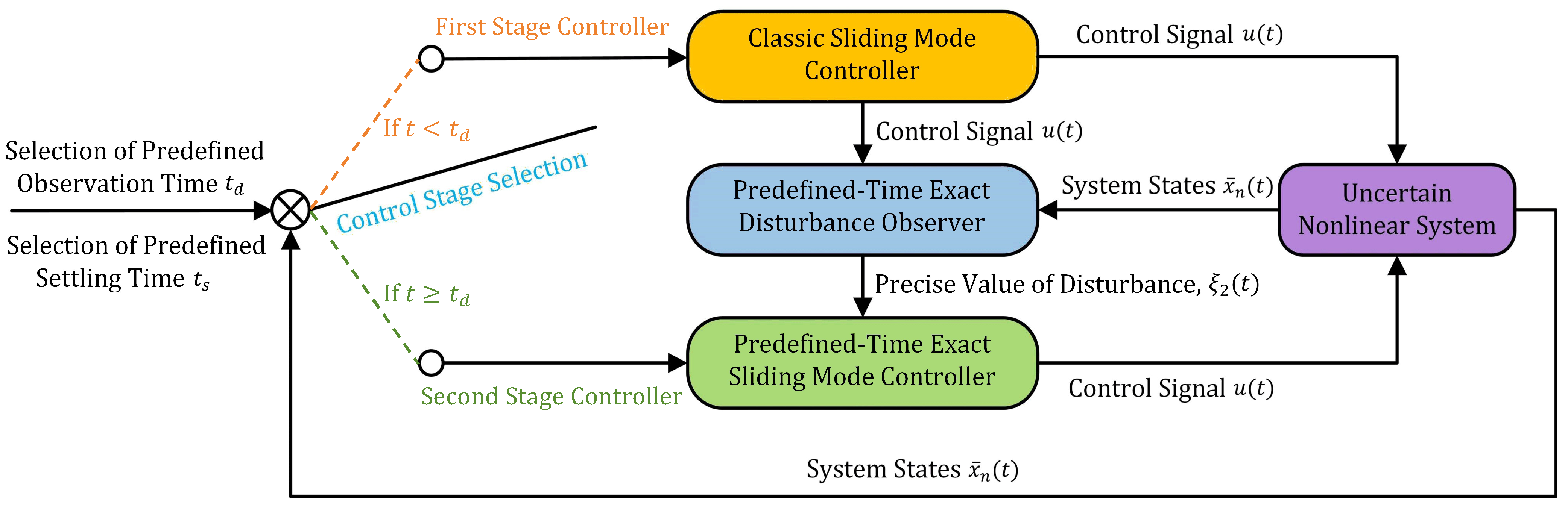
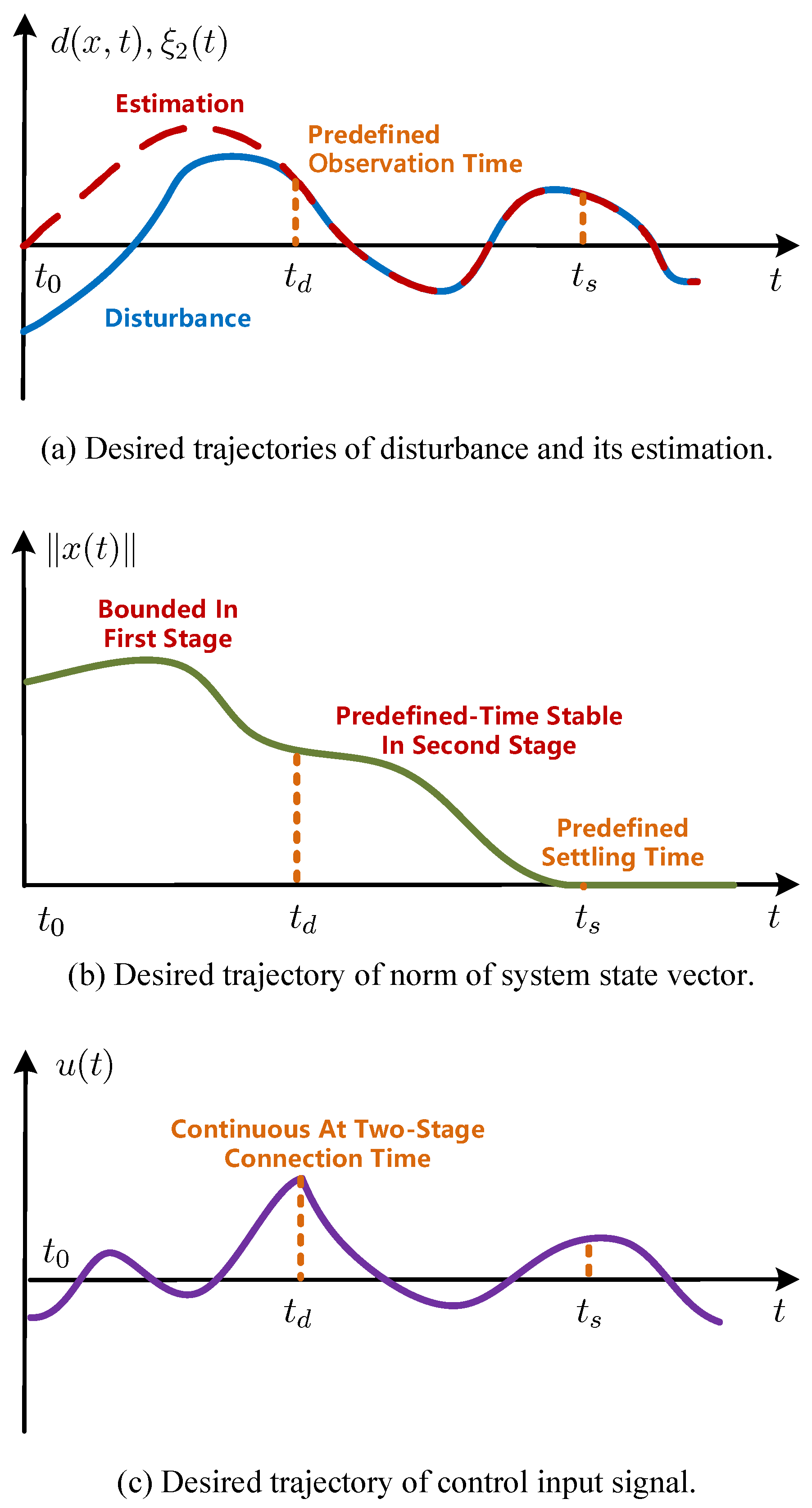
3.1. Two-Stage Control Scheme

In order to achieve the predefined-time exact control objective, the whole control stage is divided into two stages: the first stage is ${\mathbb{T}}_1=\{t:t_0\le t<t_d\}$ and the second stage is ${\mathbb{T}}_2=\{t:t\ge t_d\}$, respectively. The two-stage handover time is the predefined observation time $t_d$. Then, the structure of the two-stage predefined-time control scheme is shown in Figure 1, and the desired control result under the control scheme is illustrated in Figure 2.

In the first stage ${\mathbb{T}}_1$, predefined-time Disturbance observer (7) takes effect, generating the exact value of disturbances $d(x,t)$ with observer state ${\xi }_2\left(t\right)$ within predefined observation time $t_d$, as shown in Figure 2a. Meanwhile, controller $u\left(t\right)$ in (8) based on a classic sliding mode controller is applied, guaranteeing the boundedness of system states, as shown in Figure 2b,c.

In the second stage ${\mathbb{T}}_2$, with the exact knowledge of disturbances $d(x,t)$ provided by the predefined-time observer state ${\xi }_2\left(t\right)$ constantly, system (6) can be stabilized within the predefined settling time $t_s$ under the continuous control input signal $u\left(t\right)$ in (8) generated by a predefined-time exact sliding mode controller, as shown in Figure 2b,c.

Though the feedback control input signal $u\left(t\right)$ in (8) is continuous with respect to time in two stages, respectively, it is proven that $u\left(t\right)$ is absolutely continuous at the two-stage connection time $t_d$, as shown in Figure 2c. Thus, the control input signal under the proposed control scheme is continuous, i.e., chattering-free, essentially.

3.2. Predefined-Time Exact Disturbance Observer

Inspired by Levant’s robust finite-time sliding mode differentiator [37], we establish the structure of the new time-varying tuning function-based predefined-time exact Disturbance observer (7) as

$$\begin{array}{c}\hfill \left\{\begin{array}{c}{\dot{\xi }}_1=k_1{|\mu (t,t_d)x_n-{\xi }_1|}^{\frac{1}{2}}\mathrm{sign}(\mu (t,t_d)x_n-{\xi }_1)\hfill \\ +\dot{\mu }(t,t_d)x_n+\mu (t,t_d)f+\mu (t,t_d)bu+{\xi }_2,{\xi }_1\left(t_0\right)=0\hfill \\ {\dot{\xi }}_2=k_2\mathrm{sign}(\mu (t,t_d)x_n-{\xi }_1),{\xi }_2\left(t_0\right)=0\hfill \end{array}\right.\end{array}$$

(11)

in which $\mu :[t_0,\infty )\times (t_0,t_s)\to \mathbb{R}$ is a time-varying tuning function that satisfies the following three conditions:

Condition 1. 

There exist known constants ${\mu }_0>0$ and ${\mu }_1>0$ such that $|\mu (t,t_d)|\le {\mu }_0$ and $|\dot{\mu }(t,t_d)|\le {\mu }_1$ hold for all $t\in [t_0,\infty )$.

Condition 2. 

The initial condition $\mu (t_0,t_d)=0$ holds.

Condition 3. 

The steady condition $\mu (t,t_d)=1$ holds for all $t\in [t_d,\infty )$.

The solutions of (11) are understood in the sense of Filippov [38]. Then, we use the following theorem to analyze Observer (11):

Theorem 1. 

We consider System (6) and Observer (11). If the parameters in (11) are selected such that

$$\begin{array}{c}\hfill k_2>L,k_1>\sqrt{k_2+L}\end{array}$$

(12)

in which $L=\frac{1}{2}({\mu }_0^2+l_0^2+{\mu }_1^2+l_1^2)$, then Observer (11) can estimate $d(x,t)$ precisely within the predefined observation time $t_d$, i.e., ${\xi }_2\left(t\right)=d(x,t)$ holds for all $t\in [t_d,\infty )$.

Proof. 

We define the composite estimation errors $y_1$ and $y_2$ as

$$\begin{array}{c}\hfill \left\{\begin{array}{c}{y}_1=\mu (t,t_d)x_n-{\xi }_1\hfill \\ y_2=\mu (t,t_d)d-{\xi }_2\hfill \end{array}\right.\end{array}$$

(13)

whose dynamics can be obtained from (6) and (11) as

$$\begin{array}{c}\hfill \left\{\begin{array}{c}{\dot{y}}_1=\dot{\mu }{x}_n+\mu (f+bu+d)-k_1{\left|y_1\right|}^{\frac{1}{2}}\mathrm{sign}\left(y_1\right)-\dot{\mu }{x}_n-\mu (f+bu)-{\xi }_2\hfill \\ {\dot{y}}_2=\dot{\mu }d+\mu \dot{d}-k_2\mathrm{sign}\left(y_1\right)\hfill \end{array}\right.\end{array}$$

(14)

which yields

$$\begin{array}{c}\hfill \left\{\begin{array}{c}{\dot{y}}_1=-k_1{\left|y_1\right|}^{\frac{1}{2}}\mathrm{sign}\left(y_1\right)+y_2\hfill \\ {\dot{y}}_2=-k_2\mathrm{sign}\left(y_1\right)+\delta (t,t_d)\hfill \end{array}\right.\end{array}$$

(15)

where $\delta (t,t_d)=\dot{\mu }(t,t_d)d+\mu (t,t_d)\dot{d}$ denotes a perturbation. Applying Young’s Inequality, we have, from Assumption 2 and Condition 1, $|\delta (t,t_d)|\le \frac{1}{2}({\mu }_0^2+l_0^2+{\mu }_1^2+l_1^2)=L$ holding for all $t\in [t_0,\infty )$.

We know from (11) that the initial observer condition is set as

$$\begin{array}{c}\hfill {\xi }_1\left(t_0\right)={\xi }_2\left(t_0\right)=0\end{array}$$

(16)

and know from Condition 2 and (13) that the initial value of composite estimation errors $y_1\left(t\right)$ and $y_2\left(t\right)$ are

$$\begin{array}{c}\hfill y_1\left(t_0\right)=y_2\left(t_0\right)=0.\end{array}$$

(17)

It can be seen from Lemma 1 that System (15) is finite-time stable with parameters being selected as (12), so we know from (17) that the zero-state response of stable System (15) is

$$\begin{array}{c}\hfill y_1\left(t\right)=y_2\left(t\right)=0,t\in [t_0,\infty ).\end{array}$$

(18)

Finally, we have from (13), (18) and Condition 3

$$\begin{array}{c}\hfill {\xi }_1\left(t\right)=x_n\left(t\right),{\xi }_2\left(t\right)=d(x,t),t\in [t_d,\infty ).\end{array}$$

(19)

This ends the proof. □

Hence, Observer (11) can generate the exact value of disturbances $d(x,t)$ with state ${\xi }_2\left(t\right)$ within the predefined observation time $t_d$ and later. In the second stage ${\mathbb{T}}_2$, the exact knowledge of the real time disturbance information $d(x,t)$ from observer state ${\xi }_2\left(t\right)$ is available for control design.

Remark 4. 

The predefined observation time of Disturbance observer (11), $t_d$, is an explicit parameter in the expression of the time-varying tuning function $\mu (t,t_d)$. Time $t_d$ can be selected as an arbitrary parameter that is lesser than the final UBST $t_s$ of System (6). An example of the profile of time-varying tuning function $\mu (t,t_d)$ with $t_0=0$ and $t_d=0.5$ s is shown in Figure 3, and an example of detailed expression of $\mu (t,t_d)$ is presented in Remark 10.

Remark 5. 

A traditional finite-time disturbance observer can be obtained from Levant’s differentiator [37] as

$$\begin{array}{c}\hfill \left\{\begin{array}{c}{\dot{\xi }}_1^{\ast }=k_1{|x_n-{\xi }_1^{\ast }|}^{\frac{1}{2}}\mathrm{sign}(x_n-{\xi }_1^{\ast })+f+bu+{\xi }_2^{\ast }\hfill \\ {\dot{\xi }}_2^{\ast }=k_2\mathrm{sign}(x_n-{\xi }_1^{\ast })\hfill \end{array}\right.\end{array}$$

(20)

and the observer errors are given by

$$\left\{\begin{array}{c}{y}_1^{\ast }=x_n-{\xi }_1^{\ast }\hfill \\ y_2^{\ast }=d-{\xi }_2^{\ast }.\hfill \end{array}\right.$$

(21)

As for the traditional Observer (20), estimation errors $y_1^{\ast }\left(t\right)$ and $y_2^{\ast }\left(t\right)$ converge to zero in some finite time due to the non-zero initial error conditions $y_1^{\ast }\left(t_0\right)$ and $y_2^{\ast }\left(t_0\right)$ according to Lemma 1. As for the proposed predefined-time Observer (11), time-varying tuning function $\mu (t,t_d)$ under Condition 2 and the initial observer conditions ${\xi }_1\left(t_0\right)={\xi }_2\left(t_0\right)=0$ regulates initial composite estimation errors $y_1\left(t_0\right)=y_2\left(t_0\right)=0$. Then, the stable composite error dynamics (15) lead to $y_1\left(t\right)=y_2\left(t\right)=0$ for all $t\in [t_0,\infty )$. Since the composite estimation error $y_2\left(t\right)$ is transformed to be the real disturbance estimation error $d(x,t)-{\xi }_2\left(t\right)$ after the predefined observation time $t_d$ based on Condition 3, the result is that ${\xi }_2\left(t\right)=d(x,t)$ is obtained after $t_d$. Thus, the proposed Observer (11) generates the exact value of disturbances $d\left(t\right)$ for all $t\in [t_d,\infty )$.

3.3. First-Stage Control Design

The first stage controller $u\left(t\right)$ in ${\mathbb{T}}_1$ is designed based on classic sliding mode control via the following theorem:

Theorem 2. 

We consider System (6). The norm of system state vector $\parallel x\left(t\right)\parallel$ is bounded in the first stage ${\mathbb{T}}_1$ with the following controller:

$$\begin{array}{c}\hfill u=\frac{1}{b}\left(-{\kappa }_1{s}_1-\sum _{i=1}^{n-1}{a}_{1i}{x}_{i+1}-f\right),t\in {\mathbb{T}}_1\end{array}$$

(22)

where ${\kappa }_1>0$ is a design parameter, $s_1$ is a sliding mode function given by

$$\begin{array}{c}\hfill s_1=\sum _{i=1}^{n-1}{a}_{1i}{x}_i+x_n,t\in {\mathbb{T}}_1\end{array}$$

(23)

and $a_{1i}>0$ is a constant parameter selected such that the following matrix is Hurwitz if $n\ge 3$

$$\begin{array}{c}\hfill A_1=\left[\begin{array}{cc}{0}_{n-2}& I_{n-2}\\ -a_{11}& -a_{12}\cdots -a_{1(n-1)}\end{array}\right]\in {\mathbb{R}}^{(n-1)\times (n-1)}\end{array}$$

(24)

or $a_{11}=-A_1>0$ is a constant parameter if $n=2$.

Proof. 

We consider System (6) and define vector ${\chi }_1={[x_1,\dots ,x_{n-1}]}^T\in {\mathbb{R}}^{n-1}$. Differentiating ${\chi }_1$ with respect to time and substituting (23) into it yields

$$\begin{array}{c}\hfill {\dot{\chi }}_1=\left[\begin{array}{c}{x}_2\\ ⋮\\ x_{n-1}\\ x_n\end{array}\right]=\left[\begin{array}{c}{x}_2\\ ⋮\\ x_{n-1}\\ -\sum _{i=1}^{n-1}{a}_{1i}{x}_i+s_1\end{array}\right],t\in {\mathbb{T}}_1.\end{array}$$

(25)

It leads to

$$\begin{array}{c}\hfill {\dot{\chi }}_1=A_1{\chi }_1+B{s}_1,t\in {\mathbb{T}}_1\end{array}$$

(26)

where $B={[0_{n-2}^T,1]}^T\in {\mathbb{R}}^{n-1}$ for $n\ge 3$ or $B=1$ for $n=2$.

Then, differentiating $s_1$ with respect to time and substituting (6) into it yields

$$\begin{array}{cc}\hfill {\dot{s}}_1=& \sum _{i=1}^{n-1}{a}_{1i}{x}_{i+1}+f+bu+d,t\in {\mathbb{T}}_1.\hfill \end{array}$$

(27)

Applying (22) leads to

$$\begin{array}{c}\hfill {\dot{s}}_1=-{\kappa }_1{s}_1+d,t\in {\mathbb{T}}_1.\end{array}$$

(28)

Regarding $s_1$ as the state and d as the input of System (28), we know that unforced System (28), i.e., ${\dot{s}}_1=-{\kappa }_1{s}_1$, has a globally exponentially stable equilibrium point at origin $s_1=0$, and that System (28) is ISS in ${\mathbb{T}}_1$ according to Lemma 2, so $s_1\left(t\right)$ is bounded for all $t\in {\mathbb{T}}_1$ according to the boundedness of d in Assumption 2.

Similarly, regarding ${\chi }_1$ as the state vector and $s_1$ as the input of System (26), we know that the unforced system (26), i.e., ${\dot{\chi }}_1=A_1{\chi }_1$, has a globally exponentially stable equilibrium point at origin ${\chi }_1=0_{n-1}$, and that System (26) is ISS in ${\mathbb{T}}_1$ according to Lemma 2. Therefore, $\parallel {\chi }_1\left(t\right)\parallel$ is bounded for all $t\in {\mathbb{T}}_1$ due to the boundedness of $s_1\left(t\right)$. It indicates that $x_n\left(t\right)$ and $\parallel x\left(t\right)\parallel$ are bounded in ${\mathbb{T}}_1$ according to (23). This ends the proof. □

Hence, we can conclude from Theorem 2 that system states $x_i\left(t\right)$ are bounded in the first stage ${\mathbb{T}}_1$$(i=1,\dots ,n)$.

Remark 6. 

The first-stage control objective is to make system states signals be bounded. It is convenient to apply the simple high-order sliding mode control, i.e., the proposed first-stage controller, to achieve it. High-order finite-time sliding mode controller and some other continues control algorithms such as [36] are also available for first-stage control, but they are abandoned in this paper for simplicity.

3.4. Second-Stage Control Design

Then, a predefined-time exact sliding mode controller based on time-varying tuning function is proposed to regulate system states $x\left(t\right)$ to $0_n$ within the predefined settling time $t_s$ in the second control stage ${\mathbb{T}}_2$.

We denote the sliding mode function in the second stage ${\mathbb{T}}_2$ as $s_2(t,t_s)$, which is given by

$$\begin{array}{c}\hfill s_2(t,t_s)=\sum _{i=1}^{n-1}{a}_{2i}{\sigma }_i(t,t_s)+{\sigma }_n(t,t_s),t\in {\mathbb{T}}_2\end{array}$$

(29)

where $a_{2i}>0$ is a constant parameter selected such that the following matrix is Hurwitz if $n\ge 3$

$$\begin{array}{c}\hfill A_2=\left[\begin{array}{cc}{0}_{n-2}& I_{n-2}\\ -a_{21}& -a_{22}\cdots -a_{2(n-1)}\end{array}\right]\in {\mathbb{R}}^{(n-1)\times (n-1)}\end{array}$$

(30)

or $a_{21}=-A_2>0$ is a constant parameter if $n=2$, and ${\sigma }_j(t,t_s)\in \mathbb{R}$ are composite state variables defined as

$$\begin{array}{c}\hfill {\sigma }_j(t,t_s)=x_j-{\rho }^{(j-1)}(t,t_s),j=1,\dots ,n\end{array}$$

(31)

with $\rho :[t_d,\infty )\times (t_0,\infty )\to \mathbb{R}$ being a time-varying tuning function that fulfills the following three conditions:

Condition 4. 

${\rho }^{\left(j\right)}(t,t_s)$ are bounded and continuous with respect to time for all $t\in [t_d,\infty )$$(j=0,\dots ,n)$.

Condition 5. 

The following initial second-stage conditions hold at time $t_d$:

$$\begin{array}{cc}\hfill {\rho }^{(i-1)}(t_d,t_s)={\rho }_{i-1}:=& x_i\left(t_d\right),i=1,\dots ,n\hfill \end{array}$$

(32)

$$\begin{array}{cc}\hfill {\rho }^{\left(n\right)}(t_d,t_s)={\rho }_n:=& -{\kappa }_1\sum _{i=1}^{n-1}{a}_{1i}{x}_i\left(t_d\right)-{\kappa }_1{x}_n\left(t_d\right)+{\xi }_2\left(t_d\right)-\sum _{i=1}^{n-1}{a}_{1i}{x}_{i+1}\left(t_d\right)\hfill \end{array}$$

(33)

where ${\rho }_{i-1}\in \mathbb{R}$ and ${\rho }_n\in \mathbb{R}$ are available according to Assumption 1 and (11).

Condition 6. 

The steady condition $\rho (t,t_s)=0$ holds for all $t\in [t_s,\infty )$.

To proceed, the following theorem is utilized to design predefined-time exact sliding mode controller $u\left(t\right)$ in the second stage ${\mathbb{T}}_2$.

Theorem 3. 

We consider control input signal

$$\begin{array}{c}\hfill u=\frac{1}{b}\left(-{\kappa }_2{s}_2-\sum _{i=1}^{n-1}{a}_{2i}{\sigma }_{i+1}-f-{\xi }_2+{\rho }^{\left(n\right)}\right),t\in {\mathbb{T}}_2\end{array}$$

(34)

where ${\kappa }_2>0$ is a design parameter. Then, the solutions of System (6) are globally predefined-time stable in the second stage ${\mathbb{T}}_2$, i.e., for any $x\left(t_d\right)\in {\mathbb{R}}^n$, $x\left(t\right)=0_n$ holds for all $t\in [t_s,\infty )$, where $t_s$ is an explicit parameter in the expression of time-varying tuning function $\rho (t,t_s)$.

Proof. 

We define vector ${\chi }_2={[{\sigma }_1,\dots ,{\sigma }_{n-1}]}^T\in {\mathbb{R}}^{n-1}$. Differentiating ${\chi }_2$ with respect to time and substituting (29) into it yields

$$\begin{array}{c}\hfill {\dot{\chi }}_2=\left[\begin{array}{c}{\sigma }_2\\ ⋮\\ {\sigma }_{n-1}\\ {\sigma }_n\end{array}\right]=\left[\begin{array}{c}{\sigma }_2\\ ⋮\\ {\sigma }_{n-1}\\ -\sum _{i=1}^{n-1}{a}_{2i}{\sigma }_i+s_2\end{array}\right],t\in {\mathbb{T}}_2.\end{array}$$

(35)

It leads to

$$\begin{array}{c}\hfill {\dot{\chi }}_2=A_2{\chi }_2+B{s}_2,t\in {\mathbb{T}}_2.\end{array}$$

(36)

Then, differentiating $s_2$ with respect to time and substituting (6) and (31) into it yields

$$\begin{array}{cc}\hfill {\dot{s}}_2=& \sum _{i=1}^{n-1}{a}_{2i}{\sigma }_{i+1}+f+bu+d-{\rho }^{\left(n\right)},t\in {\mathbb{T}}_2.\hfill \end{array}$$

(37)

Applying (34) and the fact that ${\xi }_2\left(t\right)=d(x,t)$ holds for all $t\in {\mathbb{T}}_2$ in Theorem 1 leads to

$$\begin{array}{c}\hfill {\dot{s}}_2=-{\kappa }_2{s}_2,t\in {\mathbb{T}}_2.\end{array}$$

(38)

We know, from (31) and (32), that the value of composite state variables ${\sigma }_i(t,t_s)$ at the initial second-stage time $t_d$ is

$$\begin{array}{c}\hfill {\sigma }_i(t_d,t_s)=0,i=1,\dots ,n.\end{array}$$

(39)

In addition, we know from (29) that the value of sliding mode variable $s_2(t,t_s)$ at the initial second-stage time $t_d$ is

$$\begin{array}{c}\hfill s_2(t_d,t_s)=0.\end{array}$$

(40)

Then, regarding $s_2$ as the state of System (38), we determine from (40) that the zero-state response of globally asymptotic stable System (38) in the second stage is

$$\begin{array}{c}\hfill s_2(t,t_s)=0,t\in [t_d,\infty ).\end{array}$$

(41)

Moreover, regarding ${\chi }_2$ as the state vector and $s_2$ as the input of system (36), one knows from (39) and (41) that the zero-state with zero-input response of the globally asymptotic stable system (36) in the second stage is

$$\begin{array}{c}\hfill {\chi }_2\left(t\right)=0_{n-1},t\in [t_d,\infty ).\end{array}$$

(42)

Combining (29), (41), and (42) results in

$$\begin{array}{c}\hfill {\sigma }_i(t,t_s)=0,t\in [t_d,\infty ),i=1,\dots ,n.\end{array}$$

(43)

Then, Condition 6 indicates that ${\rho }^{(i-1)}(t,t_s)=0$ for all $t\in [t_s,\infty )$$(i=1,\dots ,n)$. We determine from (31) and (43) that

$$\begin{array}{c}\hfill x\left(t\right)=0_n,t\in [t_s,\infty ).\end{array}$$

(44)

Thus, the solutions of System (6) are globally predefined-time stable in the second stage ${\mathbb{T}}_2$ according to Definition 1. This ends the proof. □

Hence, system state vector $x\left(t\right)$ can converge to $0_n$ precisely within the predefined settling time $t_s$ under two-stage controller $u\left(t\right)$ in (22) and (34).

Remark 7. 

The final UBST of System (6), $t_s$, is an explicit parameter in time-varying tuning function $\rho (t,t_s)$. For instance, we consider a third-order system with initial second-stage conditions $x_1\left(t_d\right)=2$, $x_2\left(t_d\right)=-2$ and $x_3\left(t_d\right)=-3$, then an example of the profiles of time-varying tuning function $\rho (t,t_s)$ and its derivatives with $t_0=0$, $t_d=0.5$ s and $t_s=2$ s, which is shown in Figure 4. Moreover, an example of the detailed expression of $\rho (t,t_s)$ for an nth-order system is given in Remark 10.

Remark 8. 

The time-varying tuning function $\rho (t,t_s)$ regulates the initial second-stage sliding mode variable $s_2(t_d,t_s)$ and the initial second-stage composite state variables ${\sigma }_j(t_d,t_s)$ to zero $(j=1,\dots ,n)$; then, stable error dynamics (36) and (38) guarantee that $s_2(t,t_s)$ and ${\sigma }_j(t,t_s)$ are always steered at zero in $t\in [t_d,\infty )$. Finally, due to the fact that ${\sigma }_j(t,t_s)=x_j\left(t\right)$ in $t\in [t_s,\infty )$ according to (31) and Condition 6$(j=1,\dots ,n)$, we have $x_j\left(t\right)=0$ in $t\in [t_s,\infty )$.

3.5. System Analysis

It can be determined from (22) and (34) that the feedback control input signal $u\left(t\right)$ is continuous with respect to time, respectively, in two control stages. Then, the following theorem shows that it is absolutely continuous at the two-stage connection time $t_d$.

Theorem 4. 

We consider (22) and (34). Control input signal $u\left(t\right)$ is continuous with respect to time at $t=t_d$.

Proof. 

We know ${lim}_{t\to t_d^{-}}x\left(t\right)=x\left(t_d\right)$ since $x\left(t\right)$ is differentiable with respect to time. Then, we know from (22) and (23) that

$$\begin{array}{cc}\hfill \underset{t\to t_d^{-}}{lim}u\left(t\right)=& b^{-1}(x\left(t_d\right),t_d)\left(-{\kappa }_1\sum _{i=1}^{n-1}{a}_{1i}{x}_i\left(t_d\right)-{\kappa }_1{x}_n\left(t_d\right)\right.\hfill \\ \hfill & -\left.\sum _{i=1}^{n-1}{a}_{1i}{x}_{i+1}\left(t_d\right)-f(x\left(t_d\right),t_d)\right).\hfill \end{array}$$

(45)

Then, substituting (33) into (34) and considering (45) yields

$$\begin{array}{cc}u\left(t_d\right)=& b^{-1}(x\left(t_d\right),t_d)\left(-{\kappa }_2{s}_2(t_d,t_s)-\sum _{i=1}^{n-1}{a}_{2i}{\sigma }_{i+1}(t_d,t_s)-f(x\left(t_d\right),t_d)\right.\hfill \\ \hfill & \left.-{\kappa }_1\sum _{i=1}^{n-1}{a}_{1i}{x}_i\left(t_d\right)-{\kappa }_1{x}_n\left(t_d\right)-\sum _{i=1}^{n-1}{a}_{1i}{x}_{i+1}\left(t_d\right)\right)\hfill \\ \hfill =& \underset{t\to t_d^{-}}{lim}u\left(t\right)\hfill \end{array}$$

(46)

where the initial second-stage conditions $s_2(t_d,t_s)={\sigma }_i(t_d,t_s)=0$ in (39) and (40) are applied $(i=2,\dots ,n)$. Thus, the control input signal $u\left(t\right)$ is continuous with respect to time at the two-stage handover time $t_d$. This ends the proof. □

Therefore, the two-stage control input signal $u\left(t\right)$ in (22) and (34) is continuous with respect to time and chattering-free for all $t\in [t_0,\infty )$, i.e., in the whole control stage. The control input signal is piecewise continuous in form but absolutely continuous in essence.

Furthermore, the following theorem is established to show that all closed-loop system signals are bounded under the proposed control scheme for all $t\in [t_0,\infty )$.

Theorem 5. 

We consider System (6), disturbance Observer (11), first-stage control input (22) and second-stage control input (34). All closed-loop system signals are bounded for all $t\in [t_0,\infty )$.

Proof. 

It is proven in Theorem 2 that $\parallel x\left(t\right)\parallel$ and $s_1\left(t\right)$ are bounded in ${\mathbb{T}}_1$; then, we know from (22) that $u_1\left(t\right)$ is bounded in ${\mathbb{T}}_1$. Further, $\parallel x\left(t_d\right)\parallel$ is bounded since $x\left(t\right)$ is differentiable with respect to time and $x\left(t_d\right)={lim}_{t\to t_d^{-}}x\left(t\right)$.

It is proven in (18) that $y_2\left(t\right)=0$ holds in $t\in [t_0,\infty )$, so ${\xi }_2\left(t\right)$ is bounded in $t\in [t_0,\infty )$ according to (13), Assumption 2 and Condition 1.

It is proven in Theorem 3 that the trajectory of $x\left(t\right)$ is globally predefined-time stable with bounded initial second-stage condition $x\left(t_d\right)$, so $\parallel x\left(t\right)\parallel$ is bounded in ${\mathbb{T}}_2$. Then, we know that $u\left(t\right)$ is bounded in ${\mathbb{T}}_2$ from (34) and the fact that ${\sigma }_i(t,t_s)=s_2(t,t_s)=0$ in ${\mathbb{T}}_2$$(i=1,\dots ,n)$ in (41) and (43).

Finally, according to (13) and the fact that $y_1\left(t\right)=0$ for all $t\in [t_0,\infty )$ in (18), we determine from the boundedness of $x_n\left(t\right)$ in $t\in [t_0,\infty )$ and Condition 1 that ${\xi }_1\left(t\right)$ is bounded in $t\in [t_0,\infty )$. Thus, all closed-loop system signals are bounded in the whole control stage $t\in [t_0,\infty )$. □

Remark 9. 

We analyze the motivation of introducing the two time-varying tuning functions $\mu (t,t_d)$ and $\rho (t,t_s)$ under Conditions 1–6 here. $\mu (t,t_d)$ and $\dot{\mu }(t,t_d)$ are required to be bounded in Condition 1 for obtaining the boundary of perturbation $\delta (t,t_d)$ in (15). Then, Condition 2 regulates the initial composite estimation errors $y_1\left(t_0\right)$ and $y_2\left(t_0\right)$ to zero. Condition 3 makes the composite estimation error $y_2\left(t\right)$ be the real disturbance estimation error $d(x,t)-{\xi }_2\left(t\right)$ after the predefined observation time $t_d$. Moreover, ${\rho }^{\left(n\right)}(t,t_s)$ is required to be continuous and bounded in Condition 4 since it is included in control input Signal (34). Furthermore, in Condition 5, ${\rho }^{(i-1)}(t_d,t_s)$ are detailed to adjust composite variables ${\sigma }_i(t_d,t_s)$ to zero $(i=1,\dots ,n)$, and ${\rho }^{\left(n\right)}(t_d,t_s)$ is specified to guarantee the continuity of $u\left(t\right)$ at the two-stage connection time $t_d$. Finally, Condition 6 helps to transform the composite state variables ${\sigma }_i(t,t_s)$ to be the original system states $x_i\left(t\right)$ after the predefined settling time $t_s$$(i=1,\dots ,n)$.

Remark 10. 

Different candidates are available for time-varying tuning functions $\mu (t,t_d)$ and $\rho (t,t_s)$. We consider $t_0=0$ for convenience. $\mu (t,t_d)$ can be selected as the following sine function form according to Condition 1–3:

$$\begin{array}{c}\mu (t,t_d)=\left\{\begin{array}{cc}sin\left(\frac{\pi t}{2t_d}\right),\hfill & t<t_d\hfill \\ 1,\hfill & t\ge t_d.\hfill \end{array}\right.\hfill \end{array}$$

(47)

Then, constants ${\mu }_0$ and ${\mu }_1$ in Condition 1 can be selected as ${\mu }_0=1$ and ${\mu }_1=\pi /\left(2t_d\right)$, respectively. Furthermore, $\rho (t,t_s)$ can be chosen as the following polynomial form with degree $(2n+1)$ according to Condition 4–6:

$$\begin{array}{c}\rho (t,t_s)=\left\{\begin{array}{cc}\sum _{i=0}^{2n+1}{c}_i{(t-t_d)}^i,\hfill & t<t_s\hfill \\ 0,\hfill & t\ge t_s\hfill \end{array}\right.\hfill \end{array}$$

(48)

where $c_i\in \mathbb{R}$ can be obtained from the solution of a $(2n+2)$th order linear system of equations $MC=Q$, where $C={[c_{2n+1},\dots ,c_0]}^T$$\in {\mathbb{R}}^{2n+2}$, $Q={[{\rho }_0,\dots ,{\rho }_n,0_{n+1}^T]}^T\in {\mathbb{R}}^{2n+2}$, $M={[M_d,M_s]}^T\in$${\mathbb{R}}^{(2n+2)\times (2n+2)}$, $M_d\in {\mathbb{R}}^{(n+1)\times (2n+2)}$ are given by 

$$\begin{array}{c}\hfill M_d=\left[\begin{array}{ccccccc}{A}_{2n+1}^0& A_{2n}^0& \cdots & A_n^0& & \cdots & A_0^0\\ A_{2n+1}^1& A_{2n}^1& \cdots & A_n^1& \cdots & A_1^1\\ ⋮& ⋮& & ⋮& \begin{array}{c}\hfill ⋰\end{array}\\ A_{2n+1}^n& A_{2n}^n& \cdots & A_n^n\end{array}\right]\end{array}$$

(49)

and $M_s\in {\mathbb{R}}^{(n+1)\times (2n+2)}$ is given by

$$\begin{array}{cc}\hfill M_s=& \left[\begin{array}{ccc}{A}_{2n+1}^0{(t_s-t_d)}^{2n+1}& A_{2n}^0{(t_s-t_d)}^{2n}& \cdots \\ A_{2n+1}^1{(t_s-t_d)}^{2n}& A_{2n}^1{(t_s-t_d)}^{2n-1}& \cdots \\ ⋮& ⋮\\ A_{2n+1}^n{(t_s-t_d)}^{n+1}& A_{2n}^n{(t_s-t_d)}^n& \cdots \end{array}\right.\hfill \\ \hfill & \left.\begin{array}{cccc}{A}_n^0{(t_s-t_d)}^n& & \cdots & A_0^0{(t_s-t_d)}^0\\ A_n^1{(t_s-t_d)}^{n-1}& \cdots & A_1^1{(t_s-t_d)}^0\\ ⋮& \begin{array}{c}\hfill ⋰\end{array}\\ A_n^n{(t_s-t_d)}^0\end{array}\right].\hfill \end{array}$$

(50)

Remark 11. 

Now, we compare the proposed two-stage controller with a traditional two-stage chattering-free finite-time sliding mode controller [36]. We emphasize the different chattering-free control strategies in these two papers and do not analyze the difference between predefined-time and finite-time control here. In [36], in order to obtain the real time signum value, i.e., $\mathrm{sign}\left(s^{\ast }\left(t\right)\right)$, where $s^{\ast }$ denotes the unavailable sliding mode function in [36], a discrete-time procedure is constructed as (see Remark 2.3 in [36])

$$\begin{array}{cc}\hfill \mathrm{sign}\left(s^{\ast }\left(t\right)\right)=& G^{\ast }\left(t\right)-G^{\ast }(t-\tau )\hfill \end{array}$$

(51)

$$\begin{array}{cc}\hfill G^{\ast }\left(t\right)=& x_n\left(t\right)+{\int }_0^t\sum _{i=1}^n{c}_i^{\ast }{\left|x_i\left({\tau }^{\ast }\right)\right|}^{{\alpha }_i}\mathrm{sign}\left(x_i\left({\tau }^{\ast }\right)\right)\mathrm{d}{\tau }^{\ast }\hfill \end{array}$$

(52)

where $c_i^{\ast }$ and ${\alpha }_i$ are proper design parameters, and τ denotes the fundamental sample time. First, wwe can see that the initial $\mathrm{sign}\left(s^{\ast }\left(t_0\right)\right)$ may be unavailable from (51) at the initial control time. Second, $\mathrm{sign}\left(s^{\ast }\left(t\right)\right)$ updated with previous information in (51) may lag behind the actual real-time $\mathrm{sign}\left(s^{\ast }\left(t\right)\right)$. On the contrary, the proposed disturbance observer-based chattering-free control strategy is a continuous-time algorithm without any discrete-time procedure, and all variables involved are available in real time for feedback control.

Remark 12. 

Now, we compare the proposed control scheme with traditional predefined-time controller via TBG [25] when considering disturbances. According to the TBG-based control idea [25], the closed-loop dynamics under disturbances can be given by (see Equation (15) in [25])

$$\left\{\begin{array}{c}\dot{s}=-k_3{\left|s\right|}^{\frac{1}{2}}\mathrm{sign}\left(s\right)+\varrho \hfill \\ \dot{\varrho }=-k_4\mathrm{sign}\left(s\right)+\dot{d}\left(t\right)\hfill \end{array}\right.$$

(53)

where $\varrho =d+v^{\ast }$, $k_3$ and $k_4$ are positive design parameters, and

$$\begin{array}{cc}\hfill {\dot{v}}^{\ast }=& -k_4\mathrm{sign}\left(s\right)\hfill \end{array}$$

(54)

$$\begin{array}{cc}\hfill s(t,t_s)=& \sum _{i=1}^{n-1}{a}_{1i}{\sigma }_i^{\ast }(t,t_s)+{\sigma }_n^{\ast }(t,t_s),t\in [t_0,\infty )\hfill \end{array}$$

(55)

$$\begin{array}{cc}\hfill {\sigma }_i^{\ast }(t,t_s)=& x_i-{\rho }^{\ast (i-1)}(t,t_s),i=1,\dots ,n\hfill \end{array}$$

(56)

with ${\rho }^{\ast }(t,t_s)$ satisfying initial conditions ${\rho }^{\ast (i-1)}(t_0,t_s)=x_i\left(t_0\right)$ and steady condition ${\rho }^{\ast }(t,t_s)=0$ in $t\in [t_s,\infty )$. The appropriate initial condition ${\rho }^{\ast (i-1)}(t_0,t_s)$ regulates the initial sliding mode function to be $s(t_0,t_s)=0$$(i=1,\dots ,n)$, but we can hardly set the initial value $v^{\ast }\left(t_0\right)$ to make $\varrho \left(t_0\right)=0$ due to the unknown initial disturbances $d\left(t_0\right)$. Thus, System (53) with a super-twisting form reaches the equilibrium, ${[s,\varrho ]}^T=0_2$, after some finite time $t_f>t_0$. Then, the trajectories of ${\sigma }_i^{\ast }(t,t_s)$ are globally asymptotic stable under $s(t,t_s)=0$ after $t_f$ according to (55) $(i=1,\dots ,n)$, so the trajectory of $x\left(t\right)$ is asymptotic stable due to $x_i\left(t\right)={\sigma }_i^{\ast }(t,t_s)$ after the predefined settling time $t_s$. Therefore, traditional TBG-based predefined-time controller combined with super-twisting algorithm guarantees asymptotic system convergence rather than predefined-time system convergence under disturbances, as proven in Theorem 4 in [25]. However, the proposed predefined-time controller achieves zero error after predefined time $t_s$ under disturbances. It implies that the proposed controller has superiority in terms of control accuracy over a TBG-based predefined-time algorithm [25].

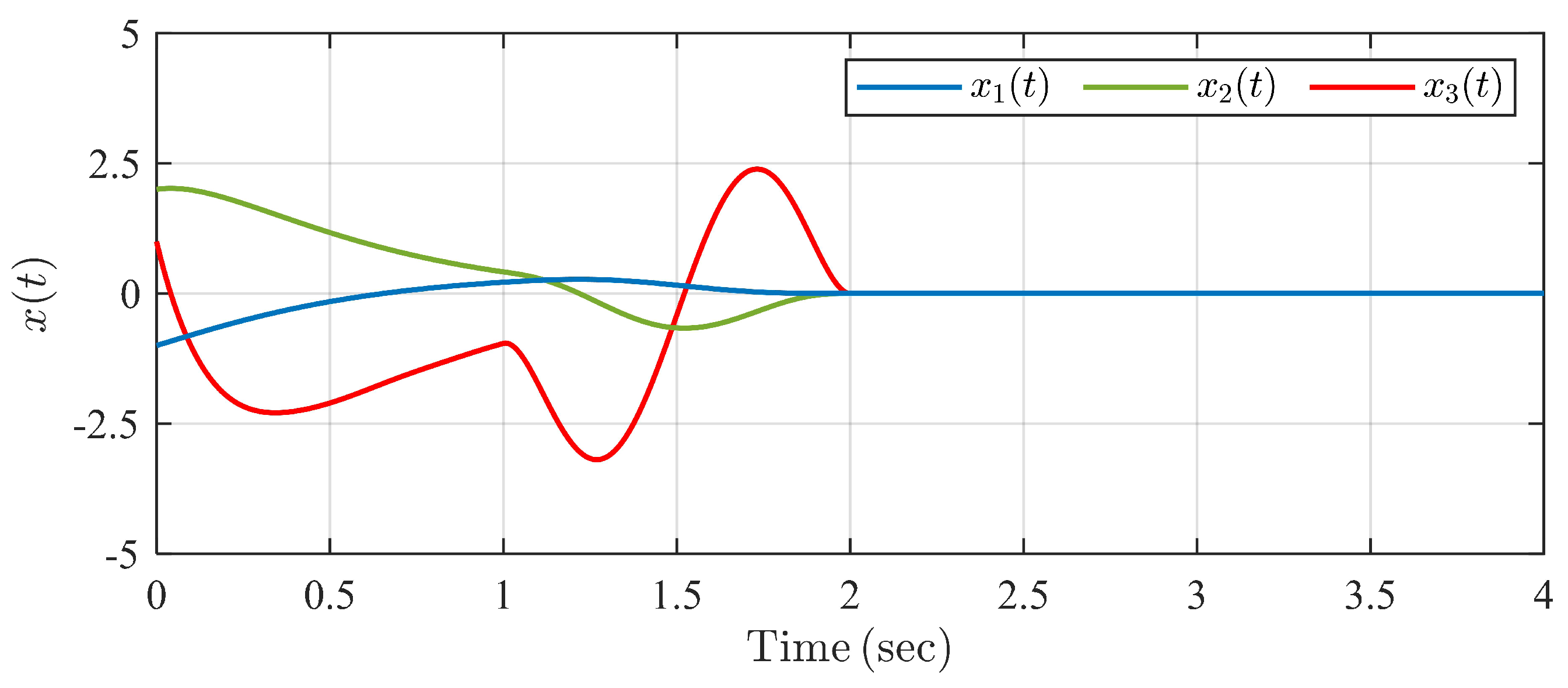
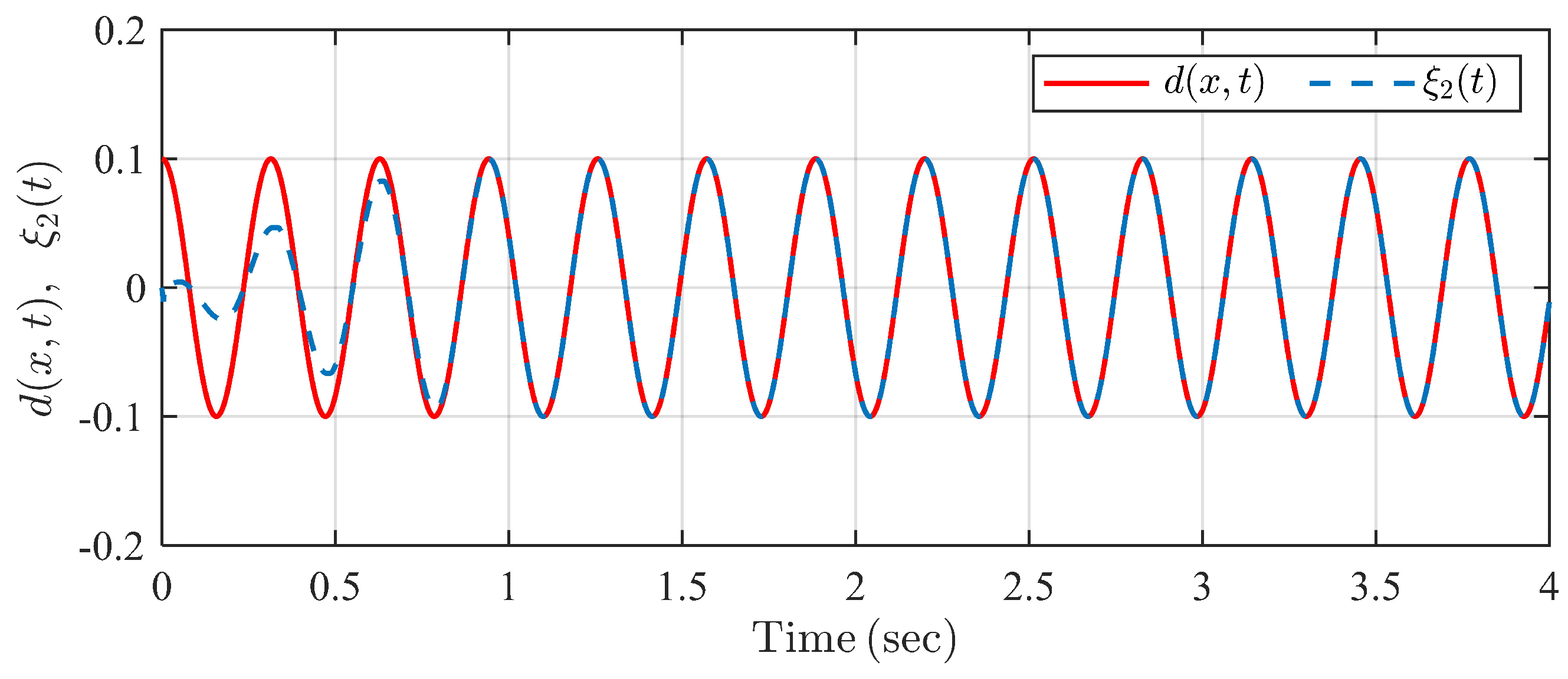
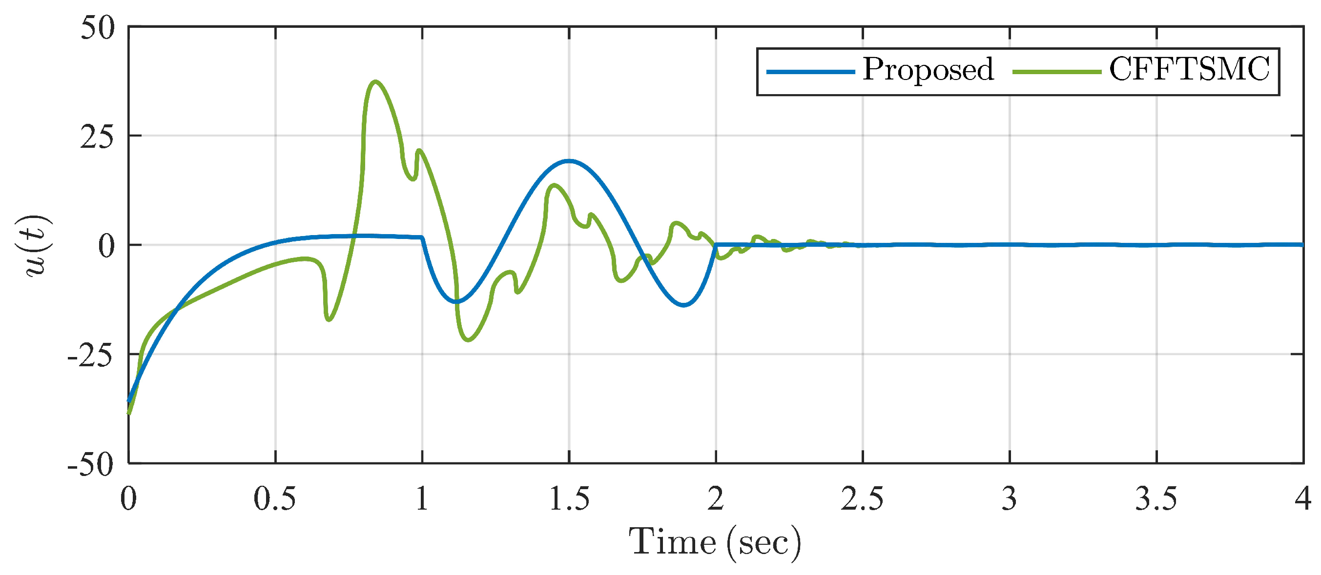
4. Simulation Examples

Two simulation examples are provided to illustrate the effectiveness of the proposed control scheme. We denote $t_0=0$ in this section for convenience.

Example 1. 

We consider the following third-order system:

$$\begin{array}{c}\hfill \left\{\begin{array}{c}{\dot{x}}_1=x_2\hfill \\ {\dot{x}}_2=x_3\hfill \\ {\dot{x}}_3=x_2^2+u+0.1cos\left(20t\right)\hfill \end{array}\right.\end{array}$$

(57)

with initial conditions $x_1\left(0\right)=-1$, $x_2\left(0\right)=2$, $x_3\left(0\right)=1$. Then, $l_0=0.1$ and $l_1=2$ can be set. The time-varying tuning functions $\mu (t,t_d)$ and $\rho (t,t_s)$ are selected as (47) and (48), respectively, with the parameters in $\rho (t,t_s)$ given by

$$\begin{array}{cc}\hfill c_7=& \frac{{\rho }_3{(t_s-t_d)}^3+12{\rho }_2{(t_s-t_d)}^2+60{\rho }_1(t_s-t_d)+120{\rho }_0}{6{(t_s-t_d)}^7}\hfill \\ \hfill c_6=& -\frac{4{\rho }_3{(t_s-t_d)}^3+45{\rho }_2{(t_s-t_d)}^2+216{\rho }_1(t_s-t_d)+420{\rho }_0}{6{(t_s-t_d)}^6}\hfill \\ \hfill c_5=& \frac{{\rho }_3{(t_s-t_d)}^3+10{\rho }_2{(t_s-t_d)}^2+45{\rho }_1(t_s-t_d)+84{\rho }_0}{{(t_s-t_d)}^5}\hfill \\ \hfill c_4=& -\frac{2{\rho }_3{(t_s-t_d)}^3+15{\rho }_2{(t_s-t_d)}^2+60{\rho }_1(t_s-t_d)+105{\rho }_0}{3{(t_s-t_d)}^4}\hfill \\ \hfill c_3=& \frac{{\rho }_3}{6},c_2=\frac{{\rho }_2}{2},c_1={\rho }_1,c_0={\rho }_0.\hfill \end{array}$$

(58)

The control parameters are chosen as ${\kappa }_1={\kappa }_2=1$, $a_{11}=a_{12}=10$, $a_{21}=a_{22}=7$, ${\mu }_0=1$, ${\mu }_1=\pi /\left(2t_d\right)$, $k_2=L+0.1$ and $k_1=\sqrt{k_2+L}+0.1$, where L is defined in Theorem 1. The predefined observation time $t_d=1\mathrm{s}$ and the predefined settling time $t_s=2\mathrm{s}$ are preset, and they appear in the expressions of $\mu (t,t_d)$ and $\rho (t,t_s)$, respectively. We also simulate System (57) under traditional chattering-free finite-time sliding mode controller (CFFTSMC) [36] for comparison. The control parameters of Example 2 in [36] are suitable for System (57).

The simulation result is shown in Figure 5, Figure 6, Figure 7 and Figure 8. It is seen in Figure 5 that system states $x_i\left(t\right)$ converge to zero within predefined settling time $2\mathrm{s}$ under the proposed controller $(i=1,2,3)$. In Figure 6, the system state trajectories are finite-time stable under CFFTSMC. However, we cannot know and adjust the settling time directly with some parameter in CFFTSMC. Figure 7 shows that the disturbance observer state ${\xi }_2\left(t\right)$ tracks unknown disturbances $d(x,t)$ within the predefined observation time $1\mathrm{s}$. Control input signals $u\left(t\right)$ are always continuous in Figure 8, but it is seen that there exist more oscillations in the control signal of CFFTSMC than in the proposed one. Thus, the simulation example verifies the effectiveness and superiority of the proposed control scheme compared with CFFTSMC.

Example 2. 

We consider the single inverted pendulum system [19]:

$$\begin{array}{c}\hfill \left\{\begin{array}{c}{\dot{z}}_1=z_2\hfill \\ {\dot{z}}_2=\frac{g_{c}sin\left(z_1\right)-m_{p}l{z}_2^{2}cos\left(z_1\right)sin\left(z_1\right)/(m_c+m_p)}{l(4/3-m_p{cos}^2\left(z_1\right)/(m_c+m_p))}\hfill \\ +\frac{cos\left(z_1\right)/(m_c+m_p)}{l(4/3-m_p{cos}^2\left(z_1\right)/(m_c+m_p))}u+d(x,t)\hfill \end{array}\right.\end{array}$$

(59)

where $z_1$ is the swing angle, $z_2$ is the swing velocity, u is the applied force, $m_c$ is the mass of the cart, $m_p$ is the mass of the pendulum, l is the length of the pendulum, $g_c=9.8m/s^2$ is the gravitational constant and d is a bounded perturbation, which may denote the wind velocity.

The objective is to solve the tracking control problem of System (59), with the desired reference signal being $r\left(t\right)$. This issue is equivalent to the stabilization problem of the following error system:

$$\left\{\begin{array}{c}{\dot{x}}_1=x_2\hfill \\ {\dot{x}}_2=f(x,t)+b(x,t)u+d(x,t)\hfill \end{array}\right.$$

(60)

where $x_1=z_1-r$, $x_2=z_2-\dot{r}$, and

$$\left\{\begin{array}{c}f=\frac{g_{c}sin(x_1+r)-m_{p}l(x_2+\dot{r}){(x_2+\dot{r})}^{2}cos(x_1+r)sin(x_1+r)/(m_c+m_p)}{l(4/3-m_p{cos}^2(x_1+r)/(m_c+m_p))}-\ddot{r}\hfill \\ b=\frac{cos(x_1+r)/(m_c+m_p)}{l(4/3-m_p{cos}^2(x_1+r)/(m_c+m_p))}\hfill \end{array}\right.$$

(61)

Then, we can apply the controller proposed in this paper for handling the tracking control issue with a predefined settling time $t_s$.

In the simulation, the parameters of the system are selected as $m_c=1\mathrm{kg}$, $m_p=0.1\mathrm{kg}$, $l=0.5\mathrm{m}$, the perturbation is given by $d=2sin\left(5t\right)+10cos\left(t\right)$, and the reference signal is $r=sin\left(0.5\pi t\right)\mathrm{rad}$. Then, $l_0=12$ and $l_1=20$ can be set. In addition, the initial system states are set as $z_1\left(0\right)=-1\mathrm{rad}$ and $z_2\left(0\right)=0\mathrm{rad}/\mathrm{s}$. Time-varying tuning functions $\mu (t,t_d)$ and $\rho (t,t_s)$ are selected as (47) and (48), respectively, with the parameters in $\rho (t,t_s)$ given by

$$\begin{array}{cc}\hfill c_5=& -\frac{{\rho }_2{(t_s-t_d)}^2+6{\rho }_1(t_s-t_d)+12{\rho }_0}{2{(t_s-t_d)}^5}\hfill \\ \hfill c_4=& \frac{3{\rho }_2{(t_s-t_d)}^2+16{\rho }_1(t_s-t_d)+30{\rho }_0}{2{(t_s-t_d)}^4}\hfill \\ \hfill c_3=& -\frac{3{\rho }_2{(t_s-t_d)}^2+12{\rho }_1(t_s-t_d)+20{\rho }_0}{2{(t_s-t_d)}^3}\hfill \\ \hfill c_2=& \frac{{\rho }_2}{2},c_1={\rho }_1,c_0={\rho }_0.\hfill \end{array}$$

(62)

The control parameters are chosen as ${\kappa }_1={\kappa }_2=1$, $a_{11}=a_{12}=10$, ${\mu }_0=1$, ${\mu }_1=\pi /\left(2t_d\right)$, $k_2=L+0.1$ and $k_1=\sqrt{k_2+L}+0.1$, where L is defined in Theorem 1. The predefined observation time $t_d=0.4\mathrm{s}$ and the predefined settling time $t_s=1\mathrm{s}$ are preset, and they appear in the expressions of $\mu (t,t_d)$ and $\rho (t,t_s)$, respectively. We also simulate System (57) under a traditional TBG predefined-time controller (TBGPTC) [25] for comparison in this example. TBGPTC can be summarized as

$$u=\frac{1}{b}\left(-k_3{\left|s\right|}^{\frac{1}{2}}\mathrm{sign}\left(s\right)-a_{11}{\sigma }_2^{\ast }(t,t_s)-f+{\ddot{\rho }}^{\ast }(t,t_s)+v^{\ast }\right)$$

(63)

where the dynamics of $v^{\ast }$ and the expressions of $s(t,t_s)$ and ${\sigma }_2^{\ast }(t,t_s)$ are shown in (54)–(56), ${\rho }^{\ast }(t,t_s)$ which can be selected as

$${\rho }^{\ast }(t,t_s)=\left\{\begin{array}{c}-\frac{x_2\left(0\right)t_s+3x_1\left(0\right)}{t_s^4}{t}^4+\frac{3x_2\left(0\right)t_s+8x_1\left(0\right)}{t_s^3}{t}^3\hfill \\ -\frac{3x_2\left(0\right)t_s+6x_1\left(0\right)}{t_s^2}{t}^2+x_2\left(0\right)t+x_1\left(0\right),\hfill & t<t_s\hfill \\ 0,\hfill & t\ge t_s\hfill \end{array}\right.$$

(64)

and $k_3=5.8$ and $k_4=11.1$ are set according to [34]. In addition, $v\left(0\right)=0$ is selected.

The simulation result is shown in Figure 9, Figure 10, Figure 11, Figure 12 and Figure 13. It can be seen from Figure 9 and Figure 10 that the swing angle $z_1\left(t\right)$ and the velocity of the single inverted pendulum system $z_2\left(t\right)$ can track reference signals $r\left(t\right)$ and $\dot{r}\left(t\right)$, respectively, within the predefined settling time $1\mathrm{s}$ under the proposed controller and TBGPTC. However, we can see in Figure 11 that there exist tracking errors after $t_s=1\mathrm{s}$ under TBGPTC, and more accurate steady tracking performance after the predefined settling time $1\mathrm{s}$ is shown by the proposed controller. In Figure 12, the predefined-time disturbance observer can generate the precise value of the system perturbation within the predefined observation time $0.4$ s. Moreover, the control input signals under two controllers are chattering-free according to the profiles in Figure 13. Thus, the proposed predefined-time controller has the advantage in the aspect of steady control accuracy compared with traditional TBGPTC.

5. Conclusions and Future Work

This paper proposes a novel two-stage chattering-free predefined-time exact sliding-mode control scheme for a class of high-order uncertain nonlinear systems with disturbances. The whole control stage is divided into two stages. A time-varying tuning function-based predefined-time exact disturbance observer is constructed, estimating the system disturbances precisely within a predefined observation time $t_d$ in the first stage $t\in [t_0,t_d)$. The classic sliding mode controller guarantees the bounded system states in the first stage, $t\in [t_0,t_d)$. Then, a time-varying tuning function-based predefined-time exact sliding mode controller stabilizes the system within a final predefined settling time $t_s>t_d$ in the second stage, $t\in [t_d,\infty )$. The continuity of the control signal with respect to time is proven, and two simulation examples show the effectiveness of the proposed control scheme. The comparison simulations indicate that the proposed control method can set the final UBST of the system compared with a traditional chattering-free finite-time sliding mode controller [36], and that the control accuracy under disturbances after the predefined settling time can be significantly improved compared with a traditional TBG-based predefined-time controller [25].

We notice that the predefined-time exact control objective is guaranteed with the usage of real-time information of system dynamics $f(x,t)$ and $b(x,t)$. In future work, the adaptive predefined-time exact control issue under uncertain dynamics $f(x,t)$ and $b(x,t)$ will be studied by developing new predefined-time parameter estimation algorithms.

References

1. Bhat, S.P.; Bernstein, D.S. Continuous finite-time stabilization of the translational and rotational double integrators. IEEE Trans. Autom. Control 1998, 43, 678–682. [Google Scholar] [CrossRef]
2. Polyakov, A. Nonlinear feedback design for fixed-time stabilization of linear control systems. IEEE Trans. Autom. Control 2012, 57, 2106–2110. [Google Scholar] [CrossRef]
3. Sánchez-Torres, J.D.; Gómez-Gutiérrez, D.; López, E.; Loukianov, A.G. A class of predefined-time stable dynamical systems. IMA J. Math. Control Inf. 2018, 35, I1–I29. [Google Scholar] [CrossRef]
4. Jiménez-Rodríguez, E.; Muñoz-Vázquez, A.J.; Sánchez-Torres, J.D.; Defoort, M.; Loukianov, A.G. A lyapunov-like characterization of predefined-time stability. IEEE Trans. Autom. Control 2020, 65, 4922–4927. [Google Scholar] [CrossRef]
5. Ferrara, A.; Incremona, G.P. Predefined-time output stabilization with second order sliding mode generation. IEEE Trans. Autom. Control 2021, 66, 1445–1451. [Google Scholar] [CrossRef]
6. Song, Y.; Ye, H.; Lewis, F.L. Prescribed-time control and its latest developments. IEEE Trans. Syst. Man, Cybern. Syst. 2023, 53, 4102–4116. [Google Scholar] [CrossRef]
7. Pal, A.K.; Kamal, S.; Nagar, S.K.; Bandyopadhyay, B.; Fridman, L. Design of controllers with arbitrary convergence time. Automatica 2020, 112, 108710. [Google Scholar] [CrossRef]
8. Song, Y.; Wang, Y.; Holloway, J.; Krstic, M. Time-varying feedback for regulation of normal-form nonlinear systems in prescribed finite time. Automatica 2017, 83, 243–251. [Google Scholar] [CrossRef]
9. Song, Y.; Wang, Y.; Krstic, M. Time-varying feedback for stabilization in prescribed finite time. Int. J. Robust Nonlinear Control 2019, 29, 618–633. [Google Scholar] [CrossRef]
10. Ye, H.; Song, Y. Prescribed-time control of uncertain strict-feedback-like systems. Int. J. Robust Nonlinear Control 2021, 31, 5281–5297. [Google Scholar] [CrossRef]
11. Singh, B.; Pal, A.K.; Kamal, S.; Dinh, T.N.; Mazenc, F. Vector control lyapunov function based stabilization of nonlinear systems in predefined time. IEEE Trans. Autom. Control 2023, 68, 4984–4989. [Google Scholar] [CrossRef]
12. Gómez-Gutiérrez, D. On the design of nonautonomous fixed-time controllers with a predefined upper bound of the settling time. Int. J. Robust Nonlinear Control 2020, 30, 3871–3885. [Google Scholar] [CrossRef]
13. Gómez-Gutiérrez, D.; Aldana-López, R.; Seeber, R.; Angulo, M.T.; Fridman, L. An arbitrary-order exact differentiator with predefined convergence time bound for signals with exponential growth bound. Automatica 2023, 153, 110995. [Google Scholar] [CrossRef]
14. Orlov, Y. Time space deformation approach to prescribed-time stabilization: Synergy of time-varying and non-lipschitz feedback designs. Automatica 2022, 144, 110485. [Google Scholar] [CrossRef]
15. Fu, L.; Ma, R.; Pang, H.; Fu, J. Predefined-time tracking of nonlinear strict-feedback systems with time-varying output constraints. J. Frankl. Inst. 2022, 359, 3492–3516. [Google Scholar] [CrossRef]
16. Ma, R.; Fu, L.; Fu, J. Prescribed-time tracking control for nonlinear systems with guaranteed performance. Automatica 2022, 146, 110573. [Google Scholar] [CrossRef]
17. Ye, H.; Song, Y. Prescribed-time tracking control of mimo nonlinear systems with nonvanishing uncertainties. IEEE Trans. Autom. Control 2023, 68, 3664–3671. [Google Scholar] [CrossRef]
18. Muñoz-Vázquez, A.J.; Sánchez-Torres, J.D.; Jiménez-Rodríguez, E.; Loukianov, A.G. Predefined-time robust stabilization of robotic manipulators. IEEE/ASME Trans. Mechatronics 2019, 24, 1033–1040. [Google Scholar] [CrossRef]
19. Sánchez-Torres, J.D.; Muñoz-Vázquez, A.J.; Defoort, M.; Jiménez-Rodríguez, E.; Loukianov, A.G. A class of predefined-time controllers for uncertain second-order systems. Eur. J. Control 2020, 53, 52–58. [Google Scholar] [CrossRef]
20. Liang, C.D.; Ge, M.F.; Liu, Z.W.; Ling, G.; Zhao, X.W. A novel sliding surface design for predefined-time stabilization of euler-lagrange systems. Nonlinear Dyn. 2021, 106, 445–458. [Google Scholar] [CrossRef]
21. Xie, S.; Chen, Q. Adaptive nonsingular predefined-time control for attitude stabilization of rigid spacecrafts. IEEE Trans. Circuits Syst. II Express Briefs 2022, 69, 189–193. [Google Scholar] [CrossRef]
22. Ding, M.; Wu, H.; Zheng, X.; Guo, Y. Adaptive predefined-time attitude stabilization control of space continuum robot. IEEE Trans. Circuits Syst. II Express Briefs 2024, 71, 647–651. [Google Scholar] [CrossRef]
23. Xu, H.; Yu, D.; Sui, S.; Chen, C.L.P. An event-triggered predefined time decentralized output feedback fuzzy adaptive control method for interconnected systems. IEEE Trans. Fuzzy Syst. 2023, 31, 631–644. [Google Scholar] [CrossRef]
24. Zhang, T.; Su, S.; Wei, W.; Yeh, R.H. Practically predefined-time adaptive fuzzy tracking control for nonlinear stochastic systems. IEEE Trans. Cybern. 2023, 53, 8000–8012. [Google Scholar] [CrossRef] [PubMed]
25. Becerra, H.M.; Vazquez, C.R.; Arechavaleta, G.; Delfin, J. Predefined-time convergence control for high-order integrator systems using time base generators. IEEE Trans. Control Syst. Technol. 2018, 26, 1866–1873. [Google Scholar] [CrossRef]
26. Chalanga, A.; Plestan, F. High-order sliding-mode control with predefined convergence time for electropneumatic actuator. IEEE Trans. Control Syst. Technol. 2021, 29, 910–917. [Google Scholar] [CrossRef]
27. Sun, L.; Liu, Y. Fixed-time adaptive sliding mode trajectory tracking control of uncertain mechanical systems. Asian J. Control 2020, 22, 2080–2089. [Google Scholar] [CrossRef]
28. Ning, B.; Han, Q.L.; Zuo, Z. Bipartite consensus tracking for second-order multiagent systems: A time-varying function-based preset-time approach. IEEE Trans. Autom. Control 2021, 66, 2739–2745. [Google Scholar] [CrossRef]
29. Liu, B.; Hou, M.; Wu, C.; Wang, W.; Wu, Z.; Huang, B. Predefined-time backstepping control for a nonlinear strict-feedback system. Int. J. Robust Nonlinear Control 2021, 31, 3354–3372. [Google Scholar] [CrossRef]
30. Lv, J.; Ju, X.; Wang, C. Neural network-based nonconservative predefined-time backstepping control for uncertain strict-feedback nonlinear systems. IEEE Trans. Neural Netw. Learn. Syst. 2023, 1–12. [Google Scholar] [CrossRef]
31. Cao, Y.; Cao, J.; Song, Y. Practical prescribed time tracking control over infinite time interval involving mismatched uncertainties and non-vanishing disturbances. Automatica 2022, 136, 110050. [Google Scholar] [CrossRef]
32. Shao, K.; Zheng, J. Predefined-time sliding mode control with prescribed convergent region. IEEE/CAA J. Autom. Sin. 2022, 9, 934–936. [Google Scholar] [CrossRef]
33. Ye, D.; Zou, A.M.; Sun, Z. Predefined-time predefined-bounded attitude tracking control for rigid spacecraft. IEEE Trans. Aerosp. Electron. Syst. 2022, 58, 464–472. [Google Scholar] [CrossRef]
34. Seeber, R.; Horn, M. Stability proof for a well-established super-twisting parameter setting. Automatica 2017, 84, 241–243. [Google Scholar] [CrossRef]
35. Khalil, H.K. Nonlinear Systems, 3rd ed.; Patience Hall: Upper Saddle River, NJ, USA, 2002. [Google Scholar]
36. Feng, Y.; Han, F.; Yu, X. Chattering free full-order sliding-mode control. Automatica 2014, 50, 1310–1314. [Google Scholar] [CrossRef]
37. Levant, A. Higher-order sliding modes, differentiation and output-feedback control. Int. J. Control 2003, 76, 924–941. [Google Scholar] [CrossRef]
38. Filippov, A.F. Differential Equations with Discontinuous Right-Hand Side; Kluwer Academic Publishing: Dordrecht, The Netherlands, 1988. [Google Scholar]
Figure 1. The structure of the two-stage control scheme.
Actuators 13 00133 g001
Figure 2. The desired control result under the proposed control scheme.
Actuators 13 00133 g002
Figure 3. An example of the profile of μ ( t , t d ) with t d = 0.5 s .
Actuators 13 00133 g003
Figure 4. An example of the profile of ρ ( t , t d ) and its derivatives with t d = 0.5 s and t s = 2 s.
Actuators 13 00133 g004
Figure 5. Trajectories of system states under the proposed controller in Example 1.
Actuators 13 00133 g005
Figure 6. Trajectories of system states under CFFTSMC in Example 1.
Actuators 13 00133 g006
Figure 7. Trajectories of disturbance and its estimation under the proposed observer in Example 1.
Actuators 13 00133 g007
Figure 8. Trajectories of control input signals for two controllers in Example 1.
Actuators 13 00133 g008
Figure 9. Trajectories of system states under the proposed controller in Example 2.
Actuators 13 00133 g009
Figure 10. Trajectories of system states under TBGPTC in Example 2.
Actuators 13 00133 g010
Figure 11. Trajectories of system errors under two controllers in Example 2.
Actuators 13 00133 g011
Figure 12. Trajectories of disturbance and its estimation under the proposed observer in Example 2.
Actuators 13 00133 g012
Figure 13. Trajectories of control input signals under two controllers in Example 2.
Actuators 13 00133 g013
Disclaimer/Publisher’s Note: The statements, opinions and data contained in all publications are solely those of the individual author(s) and contributor(s) and not of MDPI and/or the editor(s). MDPI and/or the editor(s) disclaim responsibility for any injury to people or property resulting from any ideas, methods, instructions or products referred to in the content.