Lateral Stability Control for Intelligent Commercial Vehicle Based on Reconstructed Objective Function Method

Abstract

In this paper, a novel electric-hydraulic power steering (EHPS) system and a vehicle stability coordination control algorithm are proposed which can not only ensure the accuracy of the trajectory tracking but also solve the coordination control problem between the stability of the lateral control and the stability of the roll in the extreme condition. Firstly, the EHPS system is designed to provide accurate control input of front wheel angle for vehicle lateral dynamics control. Secondly, on the basis of optimal preview theory, a new trajectory tracking fusion controller combined with sliding mode control is proposed to improve the accuracy and stability of the system in the process of vehicle lateral trajectory tracking control. Then, the stability domain boundary function of the phase plane is determined according to the phase plane of the sideslip angle-yaw rate, and the stability margin of the phase plane is calculated during the steering process. Finally, considering the tracking accuracy, lateral stability and roll stability performance in the process of trajectory tracking, the linear weighted algorithm is used to coordinate above three objectives, and the HIL bench test and real vehicle experiment verify that the proposed algorithm has good reliability and effectiveness.

1. Introduction

Under the background of the development of electric and intelligent vehicle, automatic driving technology will become a new direction for the future development of commercial vehicle. However, hydraulic power steering system is still widely used in commercial vehicle, which cannot meet the needs of the development of automatic driving technology. Since the electro-hydraulic powering steering system has the functions of active steering and active steering, it can control the vehicle active steering independently of the driver’s intention, and realize the tracking and control of the vehicle to the target trajectory under the condition of automatic driving, which is of great significance to improve the safety and stability of the automatic driving of commercial vehicle [1,2,3,4].

The accuracy of vehicle trajectory tracking and vehicle safety control are hot research topics in the field of commercial vehicle autonomous driving, including electronic stability control (ESC) and active yaw control (AYC) [5,6]. Whether in vehicle trajectory tracking control or safety control, the intelligence of steering system plays a crucial role. With the research focus of steer-by-wire (SBW) system in the field of passenger car autonomous driving becoming increasingly high, the EHPS system of commercial vehicle has attracted more and more attention from experts and scholars in recent years. In order to establish the dynamic model of EHPS system, Du et al. studied the steering ladder mechanism based on Lagrange equation and two-cylinder hydrodynamic equation, and verified the accuracy of the dynamic model through experiments [7]. Due to the interference of unknown nonlinearity, parameter uncertainty and external dynamic characteristics in actual driving scenarios, it is difficult to achieve accurate control of EHPS system for front wheel angle and path tracking. Therefore, integral sliding mode control is proposed to deal with this complex control problem, and the superiority of the method is verified by simulation experiments [8].

Vehicle track tracking generally refers to driving the vehicle body along the reference track by controlling the steering wheel angle. The reference track can be either the road center line in lane keeping control or the lane change track planned by the planning and decision level in the automatic lane change system [9,10]. In recent years, the control research on vehicle trajectory tracking is mainly concentrated in the field of nonlinear control for passenger vehicle, and there are few studies on trajectory tracking for heavy commercial vehicle. Kayacan et al. designed a lateral automatic tracking control strategy for a tractor-trailer system based on a nonlinear rolling time domain observer and nonlinear model predictive control [11]. Experiments show that the designed control strategy is superior to the traditional linear model predictive control method in tracking accuracy. Aiming at the problem of external factors interference in the process of vehicle trajectory tracking control, Ji et al. designed a vehicle lateral path tracking control strategy based on interactive robust control theory [12]. Simulation and hardware-in-the-loop experiments verify that the proposed control strategy can ensure the path tracking accuracy and lateral stability when the vehicle is disturbed by external factors. The above methods are based on the premise that the front wheel angle of the vehicle can be accurately controlled. However, in the actual control process, due to external disturbances and nonlinear factors of the system, the control effect of the control system will have a certain impact, so it is necessary to combine the sliding mode control to improve the stability of the control system [13].

With the development of autonomous driving technology, a single control target can no longer meet the actual needs. In the actual road scenario, intelligent commercial vehicles should consider multiple control objectives at the same time, such as the accuracy of trajectory tracking, the stability of lateral control, and the stability of roll, so the coordinated control problem between different control objectives has become a difficulty of research. The stability boundary of the vehicle determines the timing of the entry and exit of the vehicle stability control system, which is the basis of the vehicle stability control [14]. At present, the sideslip angle-sideslip angle rate phase plan is often used as the basis for determining the boundary of vehicle stability domain, but it only controls the sideslip angle and cannot provide a reference yaw rate threshold [15,16,17]. Although the sideslip angle-yaw rate phase plane is affected by the changes of the vehicle state parameters, its stable boundary can be easily determined and the stable boundary function is not too complicated. When dividing the boundary, the coupling degree of the stable domain and the unstable domain is low, so it is widely used in the vehicle stability controller [18,19].

The rest of this paper is organized as follows. In Section 2, the dynamics model of the EHPS system is designed and established, and the trajectory tracking fusion controller is designed. In Section 3, the boundary function of the vehicle phase plane stability domain is designed and the phase plane stability margin is calculated. On this basis, the multi-objective stability coordination control strategy is proposed. In Section 4, the simulation and experiment on the test bench and the actual vehicle are introduced in detail, and the proposed algorithms are verified. Finally, Section 5 concludes the work.

2. Materials and Methods

2.1. Dynamic Model of EHPS System

The EHPS system of commercial vehicle is a complex system integrating mechanical-electro-hydraulic coupling, which is the core component and key actuator to realize the automatic driving technology of commercial vehicles. Its nonlinear characteristics are significant, which also increases the difficulty of accurate control of the steering system. In the dynamic modeling of the EHPS system of commercial vehicle, in addition to establishing the dynamic models of the mechanical subsystem, the hydraulic subsystem and the electric subsystem, the interaction between the wheel and the ground should also be considered. Therefore, the dynamic modeling of the steering resistance system should also be carried out. The EHPS system scheme in this paper is shown in Figure 1, which is mainly composed of four parts: a mechanical system module, hydraulic system module, electric power booster system module, and a steering resistance system module.

2.1.1. Mechanical System Dynamic Model

The mechanical system model of EHPS system is mainly composed of two parts: (1) steering wheel, steering column, worm gear and worm mechanism, and circulating ball steering input; (2) Circulating ball steering input, screw nut, circulating ball steering output, steering rod system, wheels. In the autonomous driving mode, the steering controller (ECU) receives torque control instructions issued by the decision layer, and outputs the required steering torque by the steering motor to replace the hand torque imposed by the driver on the steering wheel, as shown in Figure 2. Through the above analysis, the following dynamic model of the mechanical system can be obtained:

$$J_s{\ddot{\theta }}_s+B_s{\dot{\theta }}_s+T_t+T_{fri}=T_i$$

(1)

$$M_p{\ddot{x}}_p+B_p{\dot{x}}_p+F_{fric}+F_{fres}=T_t·R_t+F_{hy}$$

(2)

$$T_t=K_t({\theta }_s-{\theta }_{lg})$$

(3)

$${\theta }_{lg}=R_t{x}_p=R_t{\theta }_f{r}_{cs}$$

(4)

where $J_s$, $M_p$, $B_s$ and $B_p$ are the moment of inertia equivalent to the steering column of steering wheel and worm gear, equivalent mass of the nut in recirculating ball, damping coefficient equivalent on to the steering column, damping coefficient between the nut and the hydraulic oil; $T_t$, $T_i$ and $T_{fri}$ are the torque measured in the TAS sensor, torque applied by the motor to steering column and the equivalent static resistance moment on steering column; $F_{fric}$, $F_{fres}$ and $F_{hy}$ are the frictional resistance in the recirculating ball, the steering resistance moment and hydraulic power; $x_p$, $R_t$ and $r_{cs}$ are the displacement of the nut, ratio of the sector gear and radius of the sector gear; ${\theta }_s$, ${\theta }_{lg}$ and ${\theta }_f$ are the steering wheel angle, sector gear angle and recirculating ball steering input shaft angle.

2.1.2. Hydraulic System

The hydraulic system schematic diagram is shown in Figure 1, which mainly includes screw and nut, rotating valves, oil tank and pump. Rotary valves are typically modelled as Wheatstone Bridges, which contain four throttle valves and the orifice area associated with the torsion rod in Figure 1. The dynamic of hydraulic system can be expressed as:

$$\left\{\begin{array}{l}{Q}_1=C_d{A}_1\sqrt{2\left(P_s-P_1\right)/\rho }-C_d{A}_3\sqrt{2P_1/\rho }=-A_P·{\dot{x}}_p+\frac{V_1}{K_{\beta }}\frac{d{p}_1}{dt}\\ Q_2=C_d{A}_2\sqrt{2\left(P_s-P_2\right)/\rho }-C_d{A}_4\sqrt{2P_2/\rho }=A_P·{\dot{x}}_p+\frac{V_2}{K_{\beta }}\frac{d{p}_2}{dt}\end{array}\right.$$

(5)

where $Q_1$ and $Q_2$ are the flows through the left and right chambers of the hydraulic cylinder; $V_1$ and $V_2$ are the volumes of the chambers at the left and right ends of the hydraulic cylinder; $C_d$ is the flow coefficient; $p_1$, $p_2$ is the pressure of the hydraulic cylinder; P_s is the inlet pressure of the rotary valve; $K_{\beta }$ is bulk modulus; $A_P$ is the piston area of the hydraulic cylinder. $A_1$-$A_4$ are the orifice area of the four rotary valves; $\rho$ is the density of liquid medium.

Through the Equation (6) hydraulic assistance can be obtained

$$F_{hy}=A_p(P_1-P_2)$$

(6)

2.1.3. Steering Load System

Different road conditions and driving scenarios will produce different steering resistance, and the EHPS system must overcome this resistance to steer. Due to the complexity of the system, it is difficult to obtain an accurate steering resistance dynamic model. In order to facilitate the analysis and control of the system, a linear spring steering resistance with front wheel angle is adopted in Equation (7).

$$F_{res}=K_s·{\theta }_f=K_s·x_p/r_{cs}$$

(7)

where $K_s$ is the stiffness coefficient between the road and the tire.

2.1.4. EHPS System Characteristic Analysis

In order to design the EHPS control system, it is necessary to analyze the dynamic characteristics of the system. According to the above analysis, EHPS system is composed of mechanical system, hydraulic system and steering resistance system. Due to the nonlinear characteristics of the hydraulic system, the entire EHPS system is also nonlinear. Under ideal conditions without considering friction, Equations (1) and (2) can be described as

$$J_s{\ddot{\theta }}_s+B_s{\dot{\theta }}_s+K_t{\theta }_s-K_t{R}_t{r}_{cs}{\theta }_f=T_i$$

(8)

$$M_p{r}_{cs}{\ddot{\theta }}_f+B_p{r}_{cs}{\dot{\theta }}_f+\left(K_r+K_t{R_t}^2{r}_{cs}\right){\theta }_f=K_t{R}_t{\theta }_s+{\mathrm{K}}_{\Psi }\Psi \left(T_t\right)$$

(9)

where, $K_{\Psi }$ is the proportional relationship between the pressure of the hydraulic system and the hydraulic power; $\Psi \left(T_t\right)$ is the relationship between the hydraulic power curve and $T_t$, ${\Psi }^{\prime }\left(T_t\right)$ is the slope of the curve at $T_t$, as shown in Figure 3.

In order to facilitate Laplace transformation of the equation, it is set as zero initial condition in this manuscript. When time $t$ = 0, input: motor torque $T_i$ = 0, output: steering wheel angle ${\theta }_s$ = 0, steering wheel speed ${\dot{\theta }}_s$ = 0, front wheel angle ${\theta }_f$ = 0, front wheel angle speed ${\dot{\theta }}_f$ = 0. The Laplace transform of Equations (8) and (9) is given as follows

$$J_s{s}^2{\theta }_s\left(s\right)+B_{s}s{\theta }_s\left(s\right)+K_t{\theta }_s\left(s\right)-K_t{R}_t{r}_{cs}{\theta }_f\left(s\right)=T_i\left(s\right)$$

(10)

$$M_p{r}_{cs}{s}^2{\theta }_f\left(s\right)+B_p{r}_{cs}s{\theta }_f\left(s\right)+\left(K_r+K_t{R_t}^2{r}_{cs}\right){\theta }_f\left(s\right)=K_t{R}_t{\theta }_s\left(s\right)+K_{\mathrm{\Psi }}{\mathrm{\Psi }}^{\prime }\left(T_t\right)$$

(11)

The transfer function of EHPS from front wheel angle to steering torque can be described as

$$\frac{{\theta }_f\left(s\right)}{T_i\left(s\right)}=\frac{{\theta }_f\left(s\right)}{{(J_s{s}^2+B_{s}s+K_t)\theta }_s\left(s\right)-K_t·R_t·r}$$

(12)

Take the parameter values in

Table 1. The parameters used in the EHPS system dynamic model.

Parameters	Values	Parameters	Values	Parameters	Values
$J_s$/(kg·m2)	0.0258	$B_p$/(Nm/s)	459	$r_{cs}$/(m)	0.05
$B_s$/(Nm·s/rad)	0.742	$M_p$/(kg)	8.07	$K_s$/(Nm/rad)	5730
$K_t$/(Nm/rad)	143.2	${\mathrm{R}}_t$	35,283	$C_d$	0.5
$K_{\beta }$/(N/m2)	1.4 × 105	$A_p$/(m2)	9.4 × 10−3	$\mathrm{\rho }$/(kg·m3)	880

and set ${\theta }_f=\delta$, the transfer function (12) can be described as

$$\frac{\delta \left(s\right)}{T_i\left(s\right)}=\frac{7020}{0.0112s^4+45.83s^3+2404s^2+282287s-2.25\times {10}^8}$$

(13)

2.2. Trajectory Tracking Fusion Controller Design

2.2.1. Optimal Preview Controller Design

Vehicle trajectory tracking control can be regarded as composed of longitudinal velocity tracking control and lateral trajectory tracking control. However, the longitudinal speed changes very little in a very short time and can generally be ignored, so the preview error of the vehicle is mainly generated by the lateral tracking control. In order to establish the relationship between preview error and steering wheel angle or front wheel angle, this paper ignores the influence of longitudinal speed change, and selects a simplified linear 2-DOF vehicle model for control, whose dynamic equation is shown as follows:

$$\left\{\begin{array}{l}\dot{\beta }=-\frac{2k_1+2k_2}{mu}\beta -\left(1+\frac{2k_1{l}_f-2k_2{l}_r}{m{u}^2}\right)\omega +\frac{2k_1}{mu}\delta \\ \dot{\omega }=-\frac{2k_1{l}_f-2k_2{l}_r}{I_z}\beta -\frac{2k_1{l_f}^2+2k_2{l_r}^2}{u{I}_z}\omega +\frac{2l_f{k}_1}{I_z}\delta \end{array}\right.$$

(14)

where $\beta$ and $\omega$ are the sideslip angle and yaw rate, respectively; $k_1$ is front cornering stiffness; $k_2$ is rear cornering stiffness; $l_f$ and $l_r$ are the distances between the front and rear axles and the vehicle gravity center, respectively; m is the vehicle mass; u is the longitudinal speed; $\delta$ is the front wheel angle; $I_z$ is the moment of inertia of the vehicle around the Z-axis.

When the vehicle speed $u$ and the front wheel angle $\delta$ are kept constant, the vehicle is in steady state at this time, that is, $\dot{\beta }=0, \dot{\omega }=0$. Putting $\dot{\omega }=0$ into the second equation in Equation (14), we can express $\omega$ in terms of $\beta$

$$\beta =-\frac{2k_1{l_f}^2+2k_2{l_r}^2}{(2k_1{l}_f-2k_2{l}_r)u}\omega +\frac{2l{k}_1{l}_f}{2k_1{l}_f-2k_2{l}_r}\delta$$

By bringing $\beta$ into the first equation in Equation (14), the relationship between $\omega$ and $\delta$ is

$$G_{\omega s}=\frac{\omega }{\delta }=\frac{2\left[\left(k_1+k_2\right)lf-\left(k_1{l}_f-k_2{l}_r\right)\right]k_{1}u}{2\left(k_1+k_2\right)(k_1{l_f}^2+k_2{l_r}^2)-(k_1{l}_f-k_2{l}_r)m{u}^2-{(k_1{l}_f-k_2{l}_r)}^2}$$

The above formula can be rewritten as

$$G_{\omega s}=\frac{\omega }{\delta }=\frac{u}{i_{s\omega }L\left(1+K{u}^2\right)}$$

(15)

where $i_{s\omega }$ is the transmission ratio between the steering wheel and the front wheel angle; $L=l_f+l_r$; K is the stability coefficient of the vehicle, which is related to the parameters of the vehicle

$$K=\frac{m\left(k_2{l}_r-k_1{l}_f\right)}{2k_1{k}_2{L}^2}$$

(16)

The gain of the sideslip angle on the steering wheel angle in the steady state is

$$G_{\beta s}=\frac{2k_2{l}_{r}L-m{u}^2{l}_f}{2i_{s\omega }{k}_2{L}^2\left(1+K{u}^2\right)}$$

(17)

It is assumed that in the future preview time, the yaw rate remains unchanged, and at this time, since the lateral velocity $v$ is much less than the longitudinal speed $u$, it can be considered that the value of the vehicle speed remains constant. Since the yaw rate remains constant, the vehicle makes a uniform circular motion within the preview time $t_p$, and velocity direction is always tangent to the driving trajectory, as shown in Figure 4.

where M is the center of the turning radius of the vehicle; G point is the position of the center of mass of the vehicle at time $t$; Point C is the predicted vehicle centroid position after preview time $t_p$; The vehicle’s running track is arc $\widehat{GC}$; $\theta$ is the center angle of the arc, $\psi$ is the heading angle, and point P is the preview point on the target trajectory. $XOY$ coordinate system is geodetic coordinate system; X_G-Y_G is the vehicle coordinate system; $∆f$ is the lateral deviation between the preview point and the current vehicle position.

As can be seen from Figure 4, $\angle CGA=\angle CGB+\beta$, and according to the string angle theorem, $\angle CGB=\theta /2$, then $\angle CGA=\theta /2+\beta$. In the triangle $∆$CGA, $y_{GC}=\mathrm{t}\mathrm{a}\mathrm{n}(\theta /2+\beta )x_{GC}$ can be obtained according to the tangent function. After time $t_p$, the ideal centroid position of the vehicle should be point P, that is, point C should coincide with point P, then $\angle PGA=\angle CGA, y_{GC}=∆f$.

According to the uniform circular motion, $\theta =\omega t_p$, and since $v\ll u$, $x_{GC}\approx u{t}_p$ can be obtained, and the ideal yaw rate can be solved by the formula ${\omega }_d={\theta /t}_p$. By $y_{GC}=\tan (\theta /2+\beta )x_{GC}$ we can obtain that $\theta$ is

$$\theta =2\left[\arctan \left(\frac{y_{GC}}{x_{GC}}\right)-\beta \right]$$

Taking $y_{GC}=∆f$, $x_{GC}\approx u{t}_p$ can be obtained

$$\theta =2\left[\arctan \left(\frac{∆f}{u{t}_p}\right)-\beta \right]$$

After the above equation is sorted out, the expected yaw rate ${\omega }_d$ can be obtained

$${\omega }_d=\frac{\theta }{t_p}=\frac{2arctan\left(∆f/\left(u{t}_p\right)\right)-2\beta }{t_p}$$

(18)

By bringing it into Equation (15), the ideal steering wheel angle can be obtained as

$${\delta }_{s\omega }^{*}=\frac{{\omega }_d}{G_{\omega s}}=\frac{2arctan\left(∆f/\left(u{t}_p\right)\right)-2\beta }{t_p{G}_{\omega s}}$$

(19)

The incremental driver direction control model (DMd) can be obtained by putting the solution of the above equation into the formula ${\delta }_{s\omega }^{*}={\delta }_{s\omega }^d+∆{\delta }_{s\omega }$ as follows

$${\delta }_{s\omega }^{*}={\delta }_{s\omega }^0+\frac{2arctan\left(∆f/\left(u{t}_p\right)\right)-2\beta -t_p{G}_{\omega s}}{t_p{G}_{\omega s}}$$

(20)

2.2.2. Trajectory Tracking Fusion Controller Based on Sliding Mode Control

When designing the optimal preview trajectory tracking controller, the control effect and stability of the controller will be greatly reduced due to the complexity, uncertainty and nonlinearity of the passenger-vehicle-road system. Therefore, based on the optimal preview control theory and sliding mode control (SMC), a new trajectory tracking fusion controller (DMd + SMC) is designed to improve the stability and rapidity of the system in the process of vehicle lateral trajectory tracking control, which combined the incremental drive direction control model (DMd) and sliding mode controller (SMC).

In the sliding mode controller designed, the difference between the actual yaw rate and the ideal yaw rate is selected as the control error $e={\omega }_r-{\omega }_d$.

The design of the sliding surface is as follows

$$s=e+{\lambda }_s{\int }_0^{t}e\left(\tau \right)d\tau$$

(21)

where ${\lambda }_s$ is the weight coefficient.

Taking the derivative of Equation (21) and combining it with the control error $e$ can be obtained

$$\dot{s}={\dot{\omega }}_r-{\dot{\omega }}_d+{\lambda }_{s}e=\frac{k_1{l}_f-k_2{l}_r}{I_z}\beta +\frac{k_1{l_f}^2+k_2{l_r}^2}{u{I}_z}{\omega }_r-\frac{l_f{k}_1}{I_z}\delta -{\dot{\omega }}_d+{\lambda }_s\left({\omega }_r-{\omega }_d\right)$$

(22)

where ${\dot{\omega }}_r$ and ${\dot{\omega }}_d$ are the real and ideal yaw angular acceleration, respectively.

The control objective of the sliding mode controller is that the sliding mode surface tends to 0, and let $\dot{s}=0$, the equivalent control law can be obtained

$$u_{eq}=-\frac{I_z}{k_1{l}_f}\left[-\frac{k_1{l}_f-k_2{l}_r}{I_z}\beta -\frac{k_1{l_f}^2+k_2{l_r}^2}{u{I}_z}{\omega }_r+{\dot{\omega }}_d-{\lambda }_s\left({\omega }_r-{\omega }_d\right)\right]$$

(23)

In order to ensure sliding mode condition of the control system under external disturbance and parameter uncertainty, an exponential reaching law $\dot{s}=-\epsilon ·sgn\left(s\right)-k·s$ is adopted, which can be obtained by combining the above formula

$$u_{req}=u_{eq}-k·sgn\left(s/\epsilon \right)$$

(24)

where, $\epsilon$ is the thickness of the boundary layer; k is the rate at which the system moving point approaches the sliding mode switching surface.

According to Lyapunov theorem, the stability analysis of the designed sliding mode controller is carried out as follows:

Theorem 1: The system defined by Equation (21) can converge to a steady state in a finite time;

Proof. 

By substituting Equations (23) and (24) into Equation (22), we can obtain

$$\begin{array}{c}\dot{s}=\frac{k_1{l}_f-k_2{l}_r}{I_z}\beta +\frac{k_1{l_f}^2+k_2{l_r}^2}{u{I}_z}{\omega }_r-\frac{l_f{k}_1}{I_z}\left[u_{eq}-k·sgn\left(s\right)\right]-{\dot{\omega }}_d+{\lambda }_s\left({\omega }_r-{\omega }_d\right)\\ =\frac{l_f{k}_1}{I_z}k·sgn\left(s\right)\hspace{1em}\hspace{1em}\hspace{1em}\hspace{1em}\hspace{1em}\hspace{1em}\hspace{1em}\hspace{1em}\hspace{1em}\hspace{1em}\hspace{1em}\end{array}$$

Define the Lyapunov function as

$$V=\frac{1}{2}{s}^2$$

The first derivative of this is solved as follows

$$\dot{V}=s·\dot{s}=\frac{l_f{k}_1}{I_z}k·sgn\left(s\right)·s$$

□

Since the above equation satisfies $sgn\left(s\right)·s\ge 0$, and the value of k satisfies the sliding mode condition $\frac{1}{2}\frac{d{s}^2}{dt}=s·\dot{s}\le -{\eta }_0\left|s\right|$, $l_f>0$; $k_1>0$; $I_z>0$, can get $\dot{V}<0$; Therefore, it shows that the system meets the stability requirement, and theorem 1 is proved.

In order to verify the control effect of the new trajectory tracking fusion controller proposed in this paper, the vehicle model and road information are built in TruckSim and Simulink environment. The trajectory tracking control effects of the two methods based on DMd and DMd + SMC are verified in the double line change condition and the three curves condition, respectively, and the simulation results are shown in Figure 5 and Figure 6.

In order to analyze the trajectory tracking accuracy under the two methods, the indexes of mean absolute error (MAE) and root mean square error (RMSE) are used to evaluate the control accuracy of the controller, and the results are shown in

Table 2. Lateral deviation of trajectory tracking under two working conditions.

Condition	Method	Max Error (m)	MAE (m)	RMSE (m)
Double line change	DMd	0.158	0.039	3.893 × 10−4
	DMd + SMC	0.076	0.017	1.722 × 10−4
Three curves	DMd	0.024	0.099	5.728 × 10−4
	DMd + SMC	0.154	0.055	3.343 × 10−4

. Compared with the trajectory tracking accuracy based on DMd model, the trajectory tracking accuracy based on DMd + SMC model is improved by 57.3% and 44.3%, respectively, under the double line change condition and the three curves condition.

2.3. Vehicle Roll Dynamics Model with Three Degrees of Freedom

In order to consider the influence of vehicle roll stability in the design of control strategy, it is necessary to take the vehicle roll freedom into account in the lateral dynamics model of commercial vehicles, and establish a 3-DOF vehicle dynamics model with yaw and roll coupling. Figure 7 shows the simplified model of the yaw-roll coupling dynamics of the heavy commercial vehicle without trailers studied in this paper, which consists of two rigid bodies, sprung mass, and unsprung mass.

Since complex vehicle dynamics models will bring great inconvenience to theoretical research and control system design, the following assumptions are made when establishing the yaw-roll coupling dynamics model:

• In steady-state steering, the influence of the steering system on the longitudinal dynamics is ignored, and the front wheel angle is taken as the input of the model;
• Assuming that the vehicle is driving on a horizontal road surface, ignoring the motion characteristics of the vehicle suspension in the vertical and pitch directions, only the simplified equivalent roll stiffness and damping coefficient are considered;
• Assume that the vehicle is driving in the linear region, and ignore the nonlinear factors of the side deviation of the tire;
• The aerodynamic effect and the effect of load changes on the tire characteristics caused by the left and right tires are ignored.

According to the above simplification and assumptions, the yaw-roll coupling dynamics of vehicles can be described by the roll moment balance equation, the lateral motion force equation and the yaw moment balance equation:

$$\left\{\begin{array}{l}\dot{\beta }=\frac{k_1}{mu}\delta -\frac{k_1+k_2}{mu}\beta +\left(\frac{k_2{l}_r-k_1{l}_f}{m{u}^2}-1\right)\omega \\ \begin{array}{l}\dot{\omega }=\frac{k_2{l}_r-k_1{l}_f}{I_z}\beta -\frac{k_1{l_f}^2+k_2{l_r}^2}{I_{z}u}\omega +\frac{k_1{l}_f}{I_z}\delta \\ \ddot{\varphi }=-\frac{h\left(k_1+k_2\right)}{J_{xeq}}\beta +\frac{h\left(k_2{l}_r-k_1{l}_f\right)}{J_{xeq}u}\omega -\frac{c}{J_{xeq}}\dot{\varphi }+\frac{mgh-k_r}{J_{xeq}}\varphi +\frac{{hk}_1}{J_{xeq}}\delta \end{array}\end{array}\right.$$

(25)

where, $I_z$ is the moment of inertia of the vehicle mass around the Z axis; $a_y$ is the lateral acceleration of the vehicle; $h$ is the distance between the center of gravity of the vehicle and the roll center; $\varphi$ is the roll angle of the vehicle; $k_r$ and $c$ are the roll stiffness and damping coefficient of suspension, respectively. $J_{xeq}$ is the moment of inertia of the vehicle mass around the roll axis.

In order to facilitate the design of the subsequent control algorithm, the above 3-DOF differential equation is expressed as a state-space equation

$$\left\{\begin{array}{l}{\dot{x}}_r=H{x}_r+F{u}_r\\ y_r=C_r{x}_r\end{array}\right.$$

(26)

where, $x_r$ is the state variable of the control system, $x_r={\left[\begin{array}{cc}\begin{array}{cc}\beta & \omega \end{array}& \begin{array}{cc}\varphi & \dot{\varphi }\end{array}\end{array}\right]}^T$; $u_r$ is the input variable of the system, and in this control system, it is the front wheel angle of the vehicle. $y_r$ is the measured output of the system, including the yaw rate of the vehicle and the roll angle rate of the vehicle, which can be obtained based on the existing on-board controller. The matrices H, F and $C_r$ are defined as follows:

$$\begin{array}{c}H=\left[\begin{array}{cc}\begin{array}{cc}-\frac{k_1+k_2}{mu}& \frac{k_2{l}_r-k_1{l}_f}{m{u}^2}-1\\ \frac{k_2{l}_r-k_1{l}_f}{I_z}& -\frac{k_1{l_f}^2+k_2{l_r}^2}{I_{z}u}\end{array}& \begin{array}{cc}0& 0\\ 0& 0\end{array}\\ \begin{array}{cc}0& 0\\ -\frac{h\left(k_1+k_2\right)}{J_{xeq}}& \frac{h\left(k_2{l}_r-k_1{l}_f\right)}{J_{xeq}u}\end{array}& \begin{array}{cc}0& 1\\ \frac{mgh-k_r}{J_{xeq}}& \frac{c}{J_{xeq}}\end{array}\end{array}\right],F=\left[\begin{array}{c}\frac{k_1}{mu}\\ \begin{array}{c}\frac{k_1{l}_f}{I_z}\\ \begin{array}{c}0\\ \frac{{hk}_1}{J_{xeq}}\end{array}\end{array}\end{array}\right],\\ C_r=\left[\begin{array}{cc}\begin{array}{cc}0& 1\end{array}& \begin{array}{cc}0& 0\end{array}\\ \begin{array}{cc}0& 0\end{array}& \begin{array}{cc}0& 1\end{array}\end{array}\right]\end{array}$$

In the actual driving condition of the vehicle, since some parameters are not easy to measure accurately, considering the dynamic roll characteristics of the suspension, the dynamic load transfer rate (LTR) is introduced to represent the roll stability of the vehicle, and its expression is shown as follows

$$LTR=-\frac{2\left(k_r\varphi +c\dot{\varphi }\right)}{mgT}=\left[\begin{array}{cc}\begin{array}{cc}0& 0\end{array}& \begin{array}{cc}-\frac{2k_r}{mgT}& -\frac{2c}{mgT}\end{array}\end{array}\right]·x_r$$

(27)

In order to verify the accuracy of the 3-DOF vehicle yaw-roll coupling dynamic model established in this paper and lay a foundation for the subsequent design of vehicle roll stability control strategy, TruckSim simulation results under different working conditions are selected and compared with the established dynamic model simulation results. The specific vehicle model parameters are shown in

Table 3. The basic parameters of simulation and comparison of roll dynamics model.

Parameters	Values	Parameters	Values	Parameters	Values
m/(kg)	5126.6	h/(m)	1.6	Jxx/(kg·m2)	10,000
ms/(kg)	78,120.2	h/(m)	1.3	lf/(m)	3.4
kr/(N/rad)	1.42 × 106	c/(N·s/rad)	9.741 × 104	lr/(m)	1.6
k1/(N/rad)	1.31 × 104	K2/(N/rad)	5.11 × 103	Iz/(kg·m2)	8249

, and the simulation results are shown in Figure 8 and Figure 9.

From Figure 8 and Figure 9, it can be seen that when the road adhesion condition is good, the output of the established yaw-roll coupling model is in good agreement with the TruckSim simulation model results, which shows that the established vehicle model can well represent the working state of the vehicle.

3. Design of Vehicle Multi-Objective Stability Coordination Control Algorithm

The vehicle stability boundary determines the intervening and exiting time of the vehicle stability control system, which is the basis of vehicle stability control. Most of the vehicle instability occurs in the nonlinear zone of the tire (that is, with the increase of the side angle of the front or rear wheels, the lateral force generated by the tire gradually tends to be saturated and the vehicle is prone to sideslip, resulting in the vehicle deviating from the driver’s expected trajectory or producing more dangerous working conditions such as tail dumping). Therefore, the stability control of the vehicle needs to focus on the stability boundary of the vehicle.

3.1. Design of Boundary Functions in Phase Plane Stability Domains

The division of stability domain in phase plane has an important influence on the stability control of vehicle, and the reasonable and accurate division of stability domain determines the time of intervention and exit of vehicle stability control system. In this paper, the phase plane of the sideslip angle-yaw rate ($\beta$-$\omega$) is used as a means to analyze the phase plane of the vehicle stability domain. By establishing the vehicle dynamics model and tire model, the phase plane of the sideslip angle-yaw rate ($\beta$-$\omega$) is drawn for analysis.

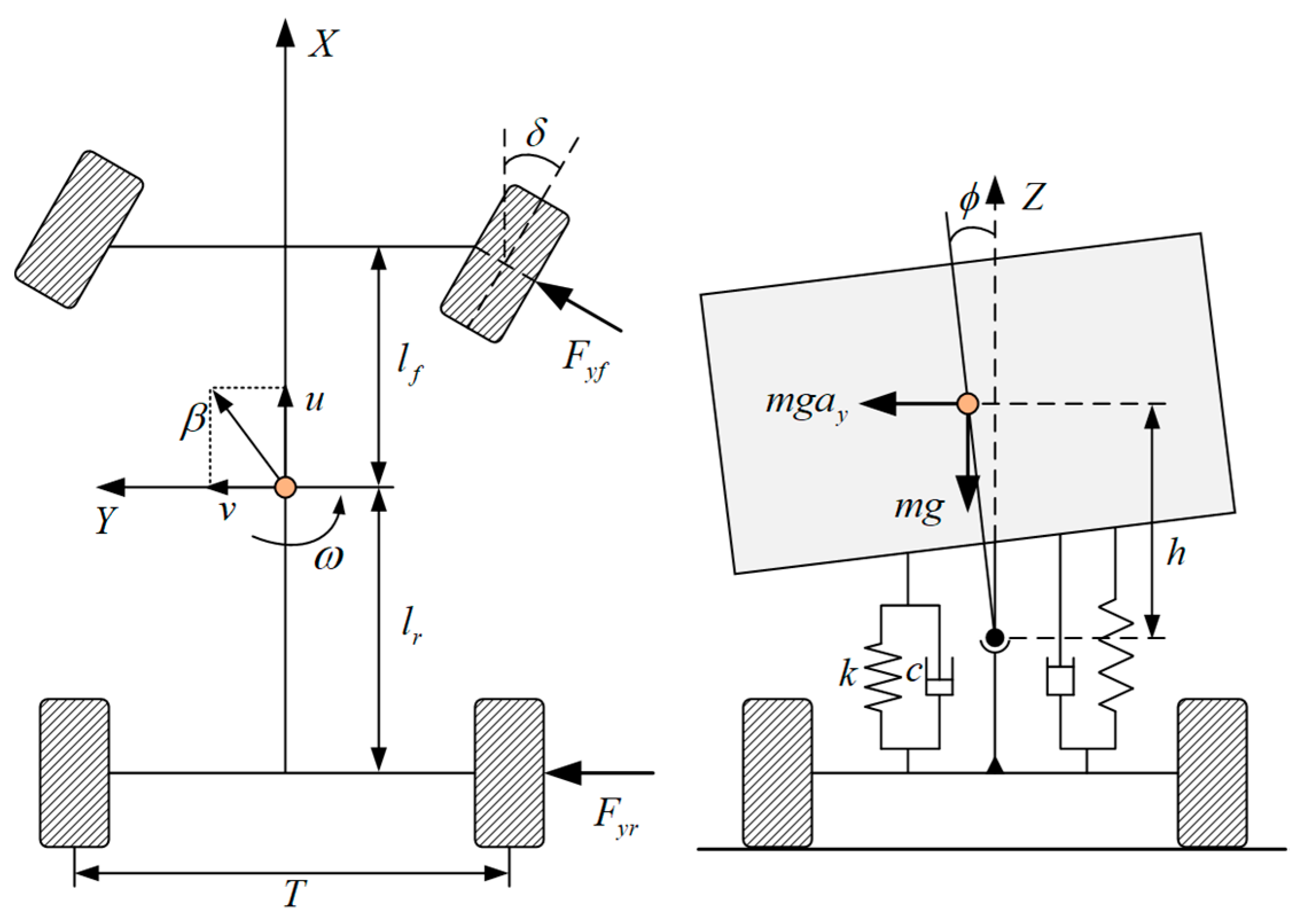
Assuming that the vehicle has a constant longitudinal velocity over a short period of time, the 2-DOF model of the vehicle with nonlinear tire force characteristics can be described by the sideslip angle-yaw rate differential equation as follows

$$\left(\begin{array}{c}\dot{\beta }\\ \dot{\omega }\end{array}\right)=f\left(\beta ,\omega ,\delta \right)=\left(\begin{array}{c}\frac{F_{yf}cos\delta +F_{yr}}{mu}cos\beta -\omega \\ \frac{{l_{f}F}_{yf}cos\delta -l_r{F}_{yr}}{I_z}\end{array}\right)$$

(28)

where $F_{yf}$ and $F_{yr}$ are the lateral deflection forces of the front and rear axes, respectively.

According to Equation (28), the equilibrium point should satisfy $x=f\left(\beta ,\omega ,\delta \right)=0$, and Matlab can be used to solve the equilibrium point and draw the plane plan of the phase trajectory.

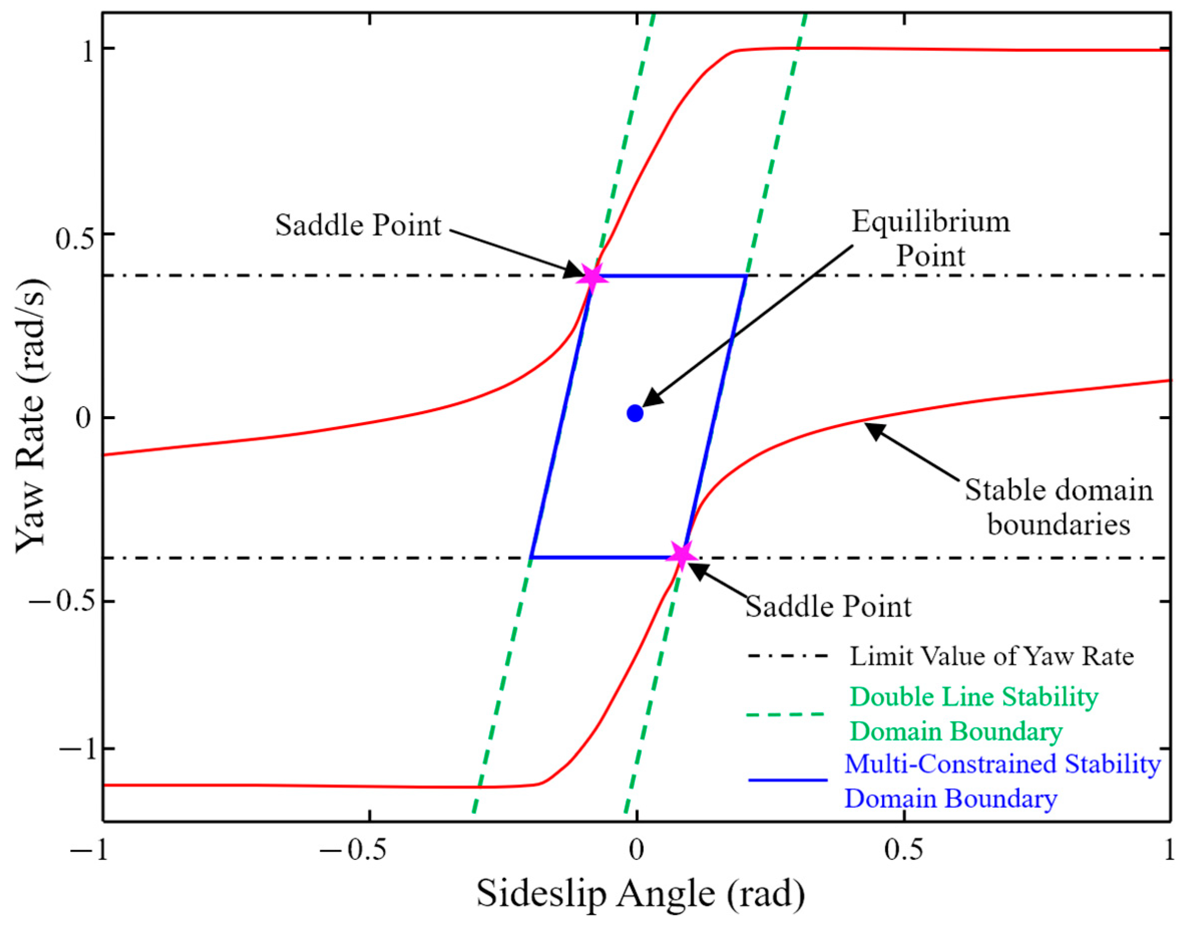
For accurate and reasonable on the phase plane stability domain, in this paper, the stability domain of the currently used classified methods such as double line method, diamond, circular and envelope method analysis summary, found that different stability domain division method has its advantages and disadvantages. Therefore, in this paper, based on double line method based on fusion the yaw rate constraint control, we put forward a kind of phase plane stability domain division method under multiple constraints, as shown in Figure 10.

Double line method by solving a saddle point of two parallel straight lines to determine the stability domain boundaries, the two saddle points has the following characteristics: (1) symmetrical about the origin of coordinates; (2) having the closest distance from the equilibrium point. The constraint of the stability domain boundary on the sideslip angle can be determined by the following expression:

$$\left|C_1\omega +\beta \right|\le C_2$$

(29)

where, $C_1$ and $C_2$ are boundary coefficients of stability domain, which are related to longitudinal vehicle speed, front wheel angle, road adhesion coefficient and other factors. The slope of the boundary is ${k=-1/C}_1$, the lateral width is ${W_h=2C}_2$, and the longitudinal width is ${W_z=2\omega }_{lim}$. The specific function of the stability domain boundary can be obtained by determining the coordinate value of the saddle point and the slope of the stability domain boundary.

The data between the longitudinal velocity, front wheel angle and road adhesion coefficient and the phase plane stability domain boundary are shown in the

Table 4. Effect of longitudinal vehicle speed on phase plane stability boundary.

Longitudinal Speed u/(km/h)	Saddle Point 1		Saddle Point 2		Slope k	Lateral Width	Longitudinal Width
	β1	ω1	β2	ω2
40	−0.13	0.71	0.13	−0.71	9.21	0.54	1.42
60	0.14	0.47	−0.14	0.47	8.12	0.44	0.94
80	0.12	0.35	−0.12	−0.35	7.31	0.41	0.71
100	0.105	0.282	−0.105	−0.282	5.72	0.38	0.564

.

According to Table 4, it can be seen that the longitudinal speed affects the lateral width of the boundary of the stability domain, and the two are negatively correlated. The function between the lateral width $W_h$ and the longitudinal speed $u$ can be obtained by fitting the data in the table as follows

$$W_h=2C_2=-3.46\times {10}^{-6}{u}^3+9.35\times {10}^{-4}{u}^2-9.12\times {10}^{-2}u+3.80$$

The relationship between the stability domain boundary coefficient $C_2$ and the longitudinal vehicle speed $u$ is

$$C_2=-1.73\times {10}^{-6}{u}^3+4.68\times {10}^{-4}{u}^2-4.56\times {10}^{-2}u+1.90$$

According to

Table 5. Effect of road adhesion coefficient on the boundary of phase plane stability boundary.

Adhesion Coefficient µ	Saddle Point 1		Saddle Point 2		Slope k	Lateral Width	Ratio of Lateral Width to Adhesion Coefficient 0.8 Kh
	β1	ω1	β2	ω2
0.2	−0.006	0.118	0.006	−0.118	0.832	0.270	0.649
0.4	−0.081	0.235	0.081	−0.235	3.907	0.282	0.678
0.6	−0.113	0.353	0.113	−0.353	4.817	0.384	0.923
0.8	−0.141	0.471	0.141	−0.471	7.977	0.416	1

, the road adhesion coefficient has a great influence on the slope $k$ and lateral width $W_h$ of the stability domain boundary. Based on the data in the table, curve fitting between slope $k$ and longitudinal vehicle speed $u$ can be obtained

$$C_1=\frac{1}{-91.98u^3+137.4u^2-72.08u+8.82}$$

Since the slope $k$ and the lateral width $W_h$ of the boundary of the stability region are also related to the longitudinal vehicle speed $u$, in order to establish the function expression of the lateral width $W_h$ and the longitudinal vehicle speed $u$ in this case, $K_h$ is defined as the ratio of the lateral width under different road adhesion and the lateral width when the adhesion coefficient is 0.8. According to the data in Table 5, the relationship between $K_h$ and $u$ can be written as

$$K_h=-8u^3+12.3u^2-5u+1.22$$

In order to establish the relationship between the offset of the longitudinal boundary and the angle of the front wheel, the value of the intersection of the stability boundary on the left and the $\beta$ axis in the phase plane is defined as ${\beta }_{-}$, and the value of the intersection of the stability boundary on the right and the $\beta$ axis in the phase plane is defined as ${\beta }_{+}$. $L_1$ is the offset of ${\beta }_{-}$ value when the front wheel angle is 0°, and $L_2$ is the offset of ${\beta }_{+}$ value when the front wheel angle is 0°, as shown in

Table 6. Effect of front wheel angle on the boundary of phase plane stability boundary.

Front Wheel Angle δ/(°)	Saddle Point 1		Saddle Point 2		Slope k	Lateral Width	Longitudinal Width
	β1	ω1	β2	ω2
−6	−0.206	0.475	0.098	−0.471	4.51	0.368	0.946
−4	−0.202	0.473	0.100	−0.474	3.21	0.564	0.946
−2	−0.172	0.471	0.108	−0.473	3.57	0.440	0.944
2	−0.108	0.472	0.171	−0.473	4.08	0.454	0.945
4	−0.045	0.472	0.211	−0.473	3.74	0.307	0.945
6	−0.079	0.475	0.207	−0.471	3.25	0.361	0.946

and

Table 7. Effect of the front wheel angle on the boundary offset of the stability boundary.

Front Wheel Angle δ/(°)	β−	Offset Relative to 0° L1	β+	Offset Relative to 0° L2
−6	−0.349	−0.055	0.189	−0.095
−4	−0.334	−0.040	0.211	−0.073
−2	−0.327	−0.033	0.251	−0.033
0	−0.294	0	0.284	0
2	−0.238	0.056	0.302	0.018
4	−0.211	0.083	0.308	0.024
6	−0.201	0.093	0.364	0.080

.

According to the data in Table 7, the offset $L_1$, $L_2$ and front wheel angle $\delta$ can be obtained by curve fitting

$$\left\{\begin{array}{l}{L}_1=1.32\times {10}^{-5}{\delta }^5-3.88\times {10}^{-5}{\delta }^4-8.36\times {10}^{-4}{\delta }^3+1.85\times {10}^{-3}{\delta }^2+0.03\delta +0.003\\ L_2=5.47\times {10}^{-6}{\delta }^5+6.7\times {10}^{-5}{\delta }^4-1.62\times {10}^{-4}{\delta }^3-2.65\times {10}^{-3}{\delta }^2+0.01\delta +0.001\end{array}\right.$$

After rearranging the above formula, the boundary function expression of the phase plane stability domain under the multi-constraint method can be obtained as

$$\left|C_1\omega +\beta +L_i\right|\le K_h{C}_2$$

(30)

where $L_i$ is the lateral offset, i = 1, 2.

3.2. Calculation of Phase Plane Stability Margin

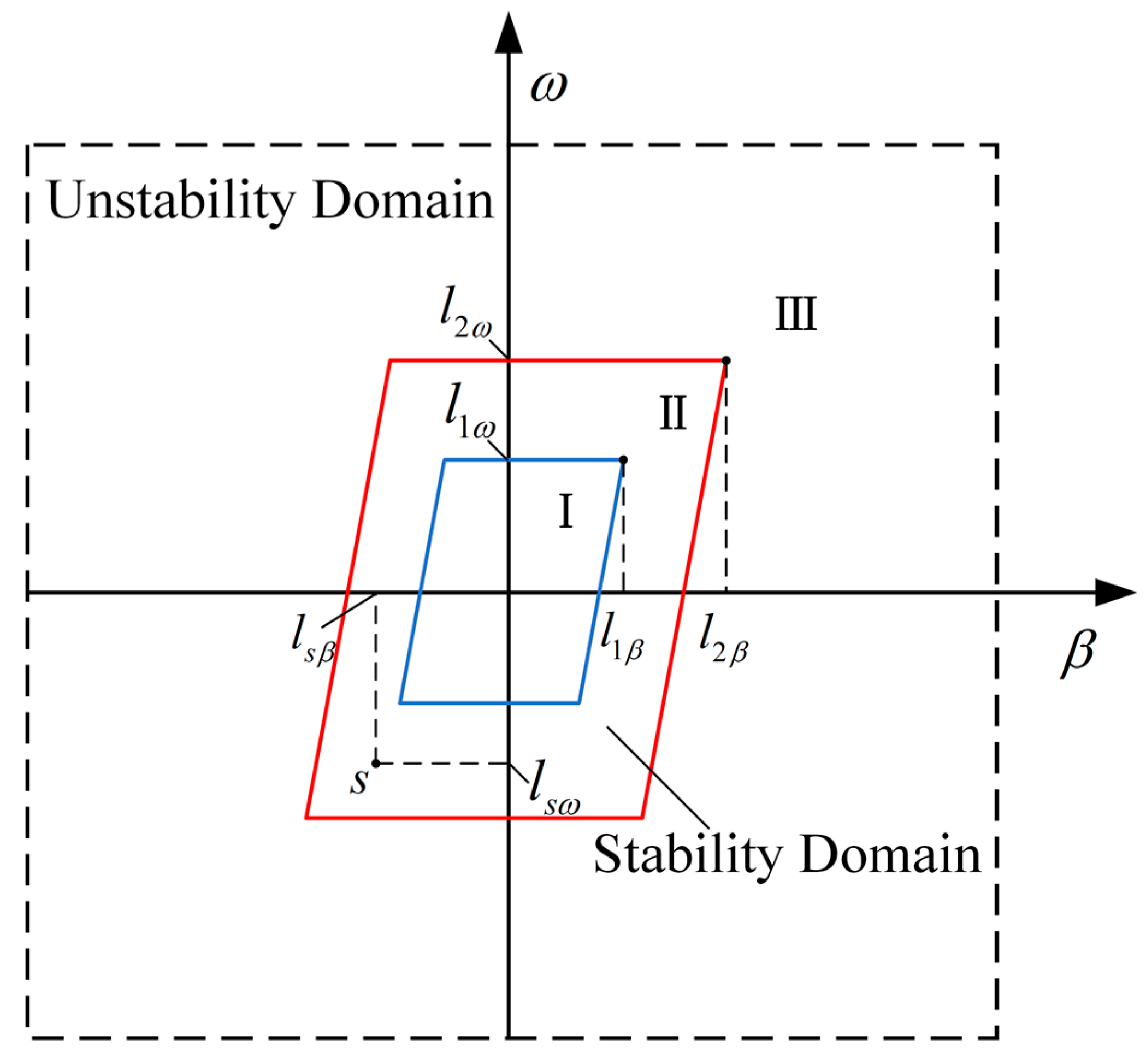
According to the above method for determining the boundary function of the stability domain of the $\beta$-$\omega$ phase plane, the stability region is divided into three parts within the determined boundary of the stability domain, which are shown in Figure 11. Any $s$ point in the stability region represents the motion state of the vehicle at the current moment, and $l_{s\omega }$ and $l_{s\beta }$ are the yaw rate value and the sideslip angle value of the vehicle at the point $s$. $l_{1\omega }, l_{2\omega }$ and $l_{1\beta }, l_{2\beta }$ are the maximum yaw rate value and the maximum sideslip angle value of the vehicle in area I and II, respectively. In this paper, considering the positions of $\omega$ and $\beta$ in the phase plane stability domain, the distance between the current state of the vehicle point $s$ and the coordinate axis is adopted as the evaluation index of the phase plane stability margin, and its value can be expressed as

$$\eta =\left\{\begin{array}{l}\frac{l_{1\beta }-l_{s\beta }}{l_{1\beta }}\times \frac{l_{1\omega }-l_{s\omega }}{l_{1\omega }},\hspace{1em}\hspace{1em}\hspace{1em}s\in \mathrm{I}\\ \begin{array}{l}\frac{l_{1\beta }-l_{s\beta }}{l_{2\beta }-l_{1\beta }}\times \frac{l_{1\omega }-l_{s\omega }}{l_{2\beta }-l_{1\beta }},\hspace{1em}\hspace{1em}\hspace{1em}s\in \mathrm{II}\\ \left|\frac{l_{s\beta }-l_{2\beta }}{l_{2\beta }}\times \frac{l_{s\omega }-l_{2\omega }}{l_{2\omega }}\right|-1,\hspace{1em}s\in \mathrm{III}\end{array}\end{array}\right.$$

(31)

According to the calculation, the value range of $\eta$ is (0, 1] when $s$ is in zone I, (−1, 0] when $s$ is in zone II, and (−2, −1] when $s$ is in zone III.

3.3. Multi-Objective Stability Coordination Control Strategy

The key of multi-objective optimization problem is how to coordinate each objective and make appropriate "compromise" between each other in order to obtain the overall optimal solution to achieve the expected goal. In order to realize the coordinated control of tracking accuracy, lateral stability and roll stability of intelligent commercial vehicle in the track tracking process, this paper combined LTR and $\beta$-$\omega$ phase plane stability domain analysis on the basis of lateral track tracking control and vehicle roll stability analysis to determine the current state of the vehicle. The linear weighted control algorithm is used to coordinate the above three objectives, and the optimal control variable of the front wheel angle is output.

The linear weighting method is a common method in the multi-objective coordinated control algorithm. It divides the importance of each sub-control objective and then transforms each sub-control objective into the following function form

$$F\left(x\right)=\sum _{i=1}^n{Q}_i{f}_i\left(x\right)$$

(32)

where, $Q_i$ is the weighted factor coefficient of each control objective, and its value reflects the importance of each sub-control objective to the whole coordinated optimization problem.

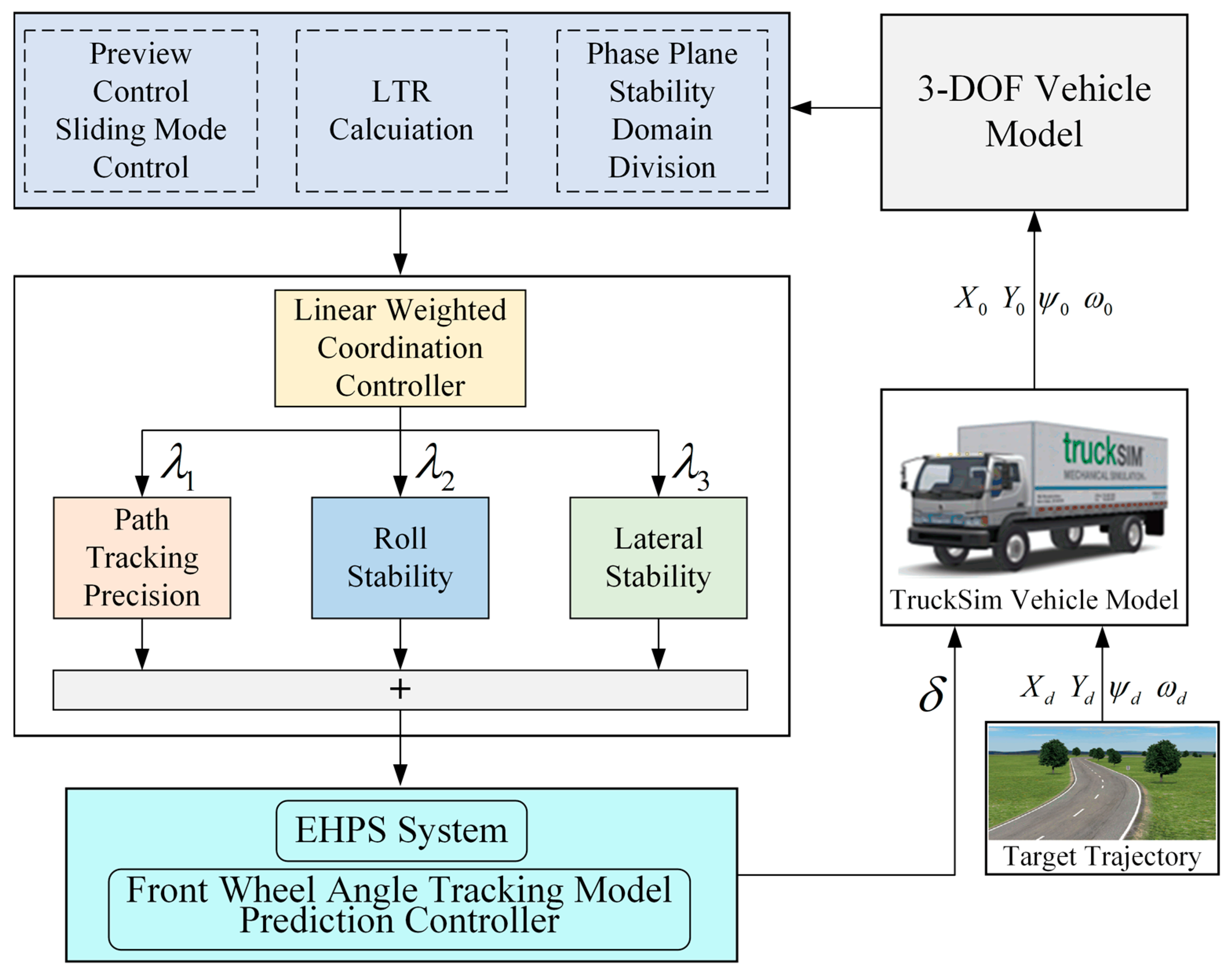
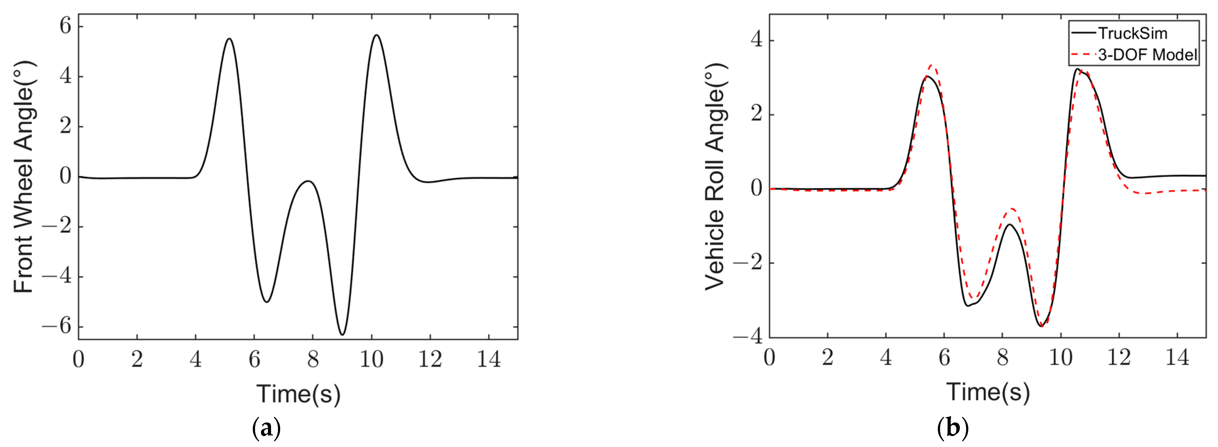
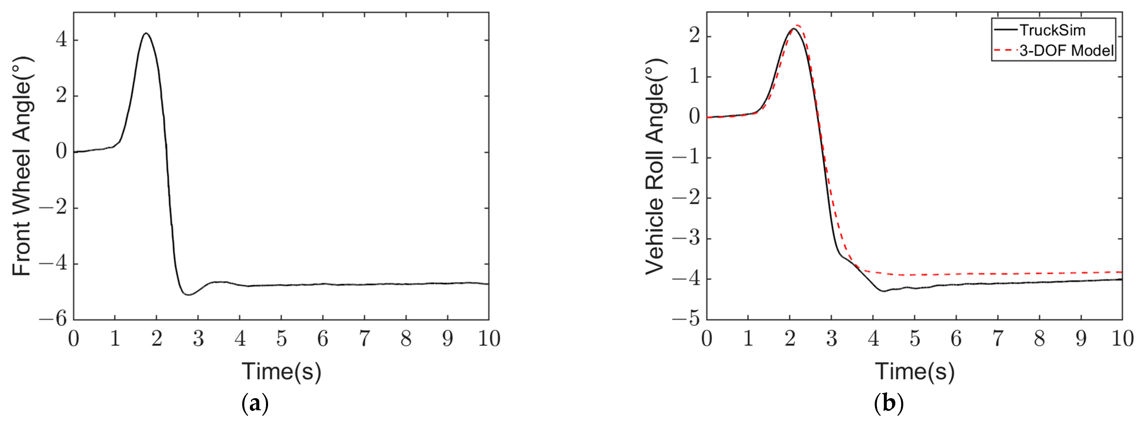
In this paper, the linear weighting algorithm is used to coordinate the control of the above three objectives, and the block diagram of the control algorithm is shown in Figure 12. The accurate tracking of the target trajectory is realized by the trajectory tracking fusion controller, and then the roll angle of the vehicle in the process of trajectory tracking is estimated by the 3-DOF model, which is used to calculate the LTR, and the lateral stability of the vehicle is calculated by using the $\beta$-$\omega$ phase plane stability domain boundary function. Finally, based on the linear weighted coordination controller, the weights of each target are assigned to determine the weights of each sub-control target, and the final control target is determined. On the basis of multiple simulations, the weight coefficients of each sub-control target are obtained in this paper, as shown in

Table 8. Linear weighted control value decision table.

LTR	Yaw Rate Increment (°/s)	Weighted Value
|LTR| ≥ 0.8	-	λ1 = 0.1, λ2 = 0.8, λ3 = 0.1
0.7 ≤ |LTR| < 0.8	|Δω| ≥ 2	λ1 = 0.2, λ2 = 0.4, λ3 = 0.4
	|Δω| < 2	λ1 = 0.4, λ2 = 0.4, λ3 = 0.2
|LTR| < 0.7	|Δω| ≥ 2	λ1 = 0.4, λ2 = 0.2, λ3 = 0.4
	|Δω| < 2	λ1 = 0.6, λ2 = 0.2, λ3 = 0.2

.

4. Results and Discussion

4.1. Simulation Results

In this paper, the vehicle, road environment and control strategy are built based on Matlab/Simulink and TruckSim to verify the effectiveness of the proposed multi-objective stability coordination control algorithm. Under the environment of vehicle speed $u$ = 65 km/h and road adhesion coefficient $\mu$ = 0.75, and vehicle speed $u$ = 50 km/h and road adhesion coefficient $\mu$ = 0.75, simulation verification is carried out for double line change conditions and three curves conditions, respectively, and the results are shown in Figure 13 and Figure 14.

It can be seen from Figure 13a,b that when DMd control is adopted, the vehicle trajectory tracking response speed is slow, and the trajectory tracking accuracy is lower than the other two control methods. The maximum lateral error is −0.41 m, which is less effective than the other two control methods within 0.1 m of the trajectory accuracy error. The two methods of non-stability (NS) control and multi-objective stability (MS) control have excellent control effects in terms of trajectory tracking accuracy, but the maximum value of LTR under DMd control is 0.23, while the maximum value of LTR under multi-objective stability control is −0.2, which can effectively suppress the state of body roll.

As can be seen from Figure 14a,b, when DMd control is adopted, the accuracy of trajectory tracking is lower than that of the other two control methods, and its maximum lateral deviation is 0.76 m, which is less effective than that of the other two control methods, whose trajectory accuracy error is within 0.24 m. The simulation results under two working conditions show that the proposed multi-objective stability control algorithm has better control effect on the trajectory tracking accuracy and stability of the vehicle.

4.2. Test Bench Results

To verify the validity of the proposed approach, a hardware-in-the-loop (HIL) test bench is constructed, as shown in Figure 15. The HIL test bench is used to simulate the real-time operation of the vehicle under various working conditions, and CAN transmit the motion state and parameters of the vehicle in TruckSim to the controller hardware system through the NI PXI communication interface (I/O, CAN, RS485, RS232) of the lower computer. After receiving these external signals in the controller, the corresponding control signals are obtained by calculating various control algorithms and control strategies to control the EHPS system and steering resistance loading system.

Figure 15 shows the HIL test results of the vehicle with a speed of $u$ = 65 km/h on the road surface with an adhesion coefficient of $\mu$ = 0.75. From Figure 16a,b, it can be seen that when only DMd control is adopted, the vehicle trajectory tracking response speed is slow, and the phenomenon of shock occurs when driving back to the straight condition, and the accuracy of trajectory tracking is lower than that of the other two control methods. The two methods have excellent control effects in the accuracy of trajectory tracking. However, the maximum value of LTR in the numerical value of lateral load transfer rate is −0.22 under the non-stability control, while the maximum value of LTR under the multi-objective stability control is −0.197. The vehicle running state is more stable with multi-objective stability control algorithm in phase plan.

Compared with the results of the simulation experiment, the steering wheel angle, lateral acceleration and LTR values in the HIL experiment all fluctuate to different degrees, which is caused by the high control frequency of the permanent magnet synchronous motor and the resistance loading motor during the experiment.

4.3. Real Vehicle Results

The multi-objective vehicle stability coordination control algorithm proposed in this paper has a greater risk of losing control when the vehicle is tested on high speed and low adhesion road surface. In order to ensure the safety of the experiment, this paper selects the road environment with low speed and high adhesion to verify the vehicle multi-objective stability coordination control algorithm under the condition of double line change track tracking. The experimental site is selected Hubei calibration matching center and real vehicle test field, and the real vehicle verification platform is shown in Figure 17.

In order to ensure the safety during the experiment, the vehicle carried out the real vehicle experiment under double line change condition on the high adhesion road surface with an adhesion coefficient of 0.85 at a speed of 40 km/h, and the results are shown in Figure 18. It can be seen from Figure 18a,b that under the conditions of low vehicle speed and high adhesion, the three control methods can all achieve accurate tracking of the lateral trajectory, and the maximum value of the lateral displacement error is very close. Figure 18c,d shows that the multi-objective stability control algorithm can better suppress the change amplitude and jitter frequency of the body roll angle and the lateral load transfer rate LTR, and improve the roll stability of the vehicle.

The MAE and RMSE results of the sum of trajectory tracking accuracy and LTR under the three control methods are shown in Figure 19. According to the calculation results, the comprehensive indexes of trajectory tracking accuracy and LTR under the multi-objective stability control are increased by 15.01% and 14.76%, respectively, compared with DMd control and non-stability control methods. The results of real vehicle experiments show that the proposed multi-objective stability control algorithm has a good control effect on the trajectory tracking accuracy and stability of the vehicle, and the effectiveness of the proposed method is verified.

5. Conclusions

In this paper, a novel EHPS system and vehicle multi-objective stability coordination control algorithm are proposed to solve the coordination control problem between the stability of the lateral control and the stability of the roll in the extreme condition. Based on theoretical analysis and experimental data, the dynamics model of EHPS system is established, and the front wheel angle tracking control algorithm is designed to provide accurate front wheel angle control input for vehicle lateral kinematics control. By combining the optimal preview theory and sliding mode control theory, a new trajectory tracking fusion controller is proposed to improve the accuracy and stability of the system in the process of vehicle lateral trajectory tracking control. Then, according to the phase plane of sideslip angle-yaw rate, the boundary function of the stability domain of the phase plane of the vehicle is determined, and the stability margin of the phase plane during the steering process is calculated. Considering the tracking accuracy, lateral stability and roll stability of the trajectory tracking process, the linear weighted algorithm is used to coordinate the control of the above three objectives. The simulation and experiment verify the designed multi-objective coordinated control algorithm, and the results show that the proposed algorithm can effectively reduce the tracking control error and improve the lateral stability of the vehicle. Therefore, the proposed controller is expected to improve the performance of intelligent commercial vehicle at the steering actuator level for autonomous driving.

References

1. Gonzalez, D.; Perez, J.; Milanes, V. A review of motion planning techniques for automated vehicles. IEEE Trans. Intell. Transp. 2016, 17, 1135–1145. [Google Scholar] [CrossRef]
2. Gordon, T.; Lidberg, J. Automated driving and autonomous functions on road vehicles. Vehicle. Syst. Dyn. 2015, 53, 958–994. [Google Scholar] [CrossRef]
3. Li, Y.; Yang, Y. Front wheel angle control for steering system of intelligent commercial vehicle based on model predictive control. IET Intell. Transp. Syst. 2023, 17, 2268–2284. [Google Scholar] [CrossRef]
4. Zhang, C.; Chu, D.; Liu, S. Trajectory planning and tracking for autonomous vehicle based on state lattice and model predictive control. IEEE Intel. Transp. Syst. 2019, 11, 29–40. [Google Scholar] [CrossRef]
5. Cheng, S.; Li, L.; Chen, J. Fusion algorithm design based on adaptive SCKF and integral correction for side-slip angle observation. IEEE Trans. Ind. Electron. 2018, 65, 5754–5763. [Google Scholar] [CrossRef]
6. Zhao, B.; Xu, N.; Chen, H.; Guo, K.; Huang, Y. Stability control of electric vehicles with in-wheel motors by considering tire slip energy. Mech. Syst. Signal Process. 2019, 118, 340–359. [Google Scholar] [CrossRef]
7. Du, H.; Zhang, Q.; Chen, S. Modeling, simulation, and experimental validation of electro-hydraulic power steering system in multi-axle vehicles. Proc. Inst. Mech. Eng. D J. Automob. Eng. 2019, 233, 317–332. [Google Scholar] [CrossRef]
8. Du, H.; Wang, L.; Chen, J. Adaptive fuzzy radial basis function neural network integral sliding mode tracking control for heavy vehicle electrohydraulic power steering systems. Proc. Inst. Mech. Eng. D J. Automob. Eng. Min. J. 2020, 234, 872–886. [Google Scholar] [CrossRef]
9. Wang, R.; Ye, Q.; Cai, Y. Analyzing the influence of automatic steering system on the trajectory tracking accuracy of intelligent vehicle. Adv. Eng. Softw. 2018, 121, 188–196. [Google Scholar] [CrossRef]
10. Liu, Y.; Ji, X.; Yang, K. Finite-time optimized robust control with adaptive state estimation algorithm for autonomous heavy vehicle. Mech. Syst. Signal Process. 2020, 139, 106616. [Google Scholar] [CrossRef]
11. Kayacan, E.; Saeys, W.; Ramon, H. Experimental validation of linear and nonlinear MPC on an articulated unmanned ground vehicle. IEEE/ASME Trans. Mechatron. 2018, 23, 2023–2030. [Google Scholar] [CrossRef]
12. Ji, X.; Liu, Y.; He, X. Interactive control paradigm-based robust lateral stability controller design for autonomous automobile path tracking with uncertain disturbance: A dynamic game approach. IEEE Trans. Veh. Technol. 2018, 67, 6906–6920. [Google Scholar] [CrossRef]
13. Esmaeili, N.; Kazemi, R.; Oreh, S. An adaptive slide mode controller for the lateral control of articulated long vehicles. Proc. Inst. Mech. Eng. Part K J. Multi-Body Dyn. 2019, 233, 487–515. [Google Scholar]
14. Xiong, L.; Yu, Z.; Wang, Y.; Yang, C.; Meng, Y. Vehicle dynamics control of four in-wheel motor drive electric vehicle using gain scheduling based on tyre cornering stiffness estimation. Veh. Syst. Dyn. 2021, 50, 831–846. [Google Scholar] [CrossRef]
15. Guo, L.; Ge, P.; Sun, D. Torque distribution algorithm for stability control of electric vehicle driven by four in-wheel motors under emergency conditions. IEEE Access 2019, 7, 104737–104748. [Google Scholar] [CrossRef]
16. Ono, E.; Hosoe, S.; Tuan, H.D. Bifurcation in Vehicle Dynamics and Robust Front Wheel Steering Control. IEEE Trans. Control. Syst. Technol. 1998, 6, 412–420. [Google Scholar] [CrossRef]
17. Bobier-Tiu, C.G.; Beal, C.E.; Kegelman, J.C. Vehicle control synthesis using phase portraits of planar dynamics. Veh. Syst. Dyn. 2018, 57, 1318–1337. [Google Scholar] [CrossRef]
18. Shen, S.; Wang, J.; Shi, P.; Premier, G. Nonlinear dynamics and stability analysis of vehicle plane motions. Veh. Syst. Dyn. 2007, 45, 15–35. [Google Scholar] [CrossRef]
19. Erlien, S.M.; Fujita, S.; Gerdes, J.C. Shared steering control using safe envelopes for obstacle avoidance and vehicle stability. IEEE Trans. Intell. Transp. Syst. 2016, 17, 441–451. [Google Scholar] [CrossRef]
Figure 1. Schematic diagram of the EHPS system.
Actuators 13 00134 g001
Figure 2. Schematic diagram of the EHPS mechanical system.
Actuators 13 00134 g002
Figure 3. Schematic diagram of hydraulic assist curve.
Actuators 13 00134 g003
Figure 4. Prediction diagram of vehicle trajectory at constant yaw rate.
Actuators 13 00134 g004
Figure 5. The simulation results of double line change at u = 65 km/h, μ = 0.75: (a) Lateral displacement of vehicle; (b) Lateral displacement error of vehicle.
Actuators 13 00134 g005
Figure 6. The simulation results of three curves at u = 65 km/h, μ = 0.75: (a) Lateral displacement of vehicle; (b) Lateral displacement error of vehicle.
Actuators 13 00134 g006
Figure 7. The 3-DOF vehicle yaw-roll coupling dynamic model.
Actuators 13 00134 g007
Figure 8. Simulation results of high-speed and high-adhesion double line change condition at u = 75 km/h, μ = 0.85: (a) Front wheel angle; (b) Vehicle roll angle.
Actuators 13 00134 g008
Figure 9. Simulation results of high-speed and high-adhesion fishing hook condition at u = 75 km/h, μ = 0.85: (a) Front wheel angle; (b) Vehicle roll angle.
Actuators 13 00134 g009
Figure 10. Comparison of double line method and multiple constraint method.
Actuators 13 00134 g010
Figure 11. β - ω phase plane stability domain partition.
Actuators 13 00134 g011
Figure 12. Multi-objective coordinated stability control strategy diagram.
Actuators 13 00134 g012
Figure 13. Simulation results of high-speed and high-adhesion double line change condition at u = 65 km/h, μ = 0.75: (a) Lateral displacement of vehicle; (b) Lateral displacement error of vehicle; (c) LTR; (d) β - ω phase plane contrast.
Actuators 13 00134 g013
Figure 14. Simulation results of low-speed and low-adhesion three curves condition at u = 50 km/h, μ = 0.75: (a) Lateral displacement of vehicle; (b) Lateral displacement error of vehicle; (c) LTR; (d) β - ω phase plane contrast.
Actuators 13 00134 g014aActuators 13 00134 g014b
Figure 15. Structure of hardware-in-the-loop test bench.
Actuators 13 00134 g015
Figure 16. Simulation results of high-speed and low-adhesion single line change condition at u = 65 km/h, μ = 0.75: (a) Lateral displacement of vehicle; (b) Lateral displacement error of vehicle; (c) LTR; (d) β - ω phase plane contrast.
Actuators 13 00134 g016aActuators 13 00134 g016b
Figure 17. Real vehicle test platform of EHPS system.
Actuators 13 00134 g017
Figure 18. Simulation results of low-speed and high-adhesion double line change condition at u = 40 km/h, μ = 0.85: (a) Lateral displacement of vehicle; (b) Lateral displacement error of vehicle; (c) LTR; (d) β - ω phase plane contrast.
Actuators 13 00134 g018
Figure 19. Comparison of the sum of lateral error and LTR value.
Actuators 13 00134 g019