Augmented Kalman Estimator and Equivalent Replacement Based Taylor Series-LQG Control for a Magnetorheological Semi-Active Suspension

Abstract

This research presents an augmented Kalman estimator and an equivalent replacement-based Taylor series (ERBTS)-linear quadratic Gaussian (LQG) control strategy to cope with the control accuracy and response delay of magnetorheological (MR) dampers for vehicle semi-active suspensions. The parameters in the MR model are identified from experimental measurements. Then, two main sources of control error, namely, modelling error and real-time variety of the MR damper output force, are defined as an integrated compound real-time variety. Subsequently, they are written into a differential equation with characteristics of the minimum system to augment the state equation of the semi-active suspension system. The augmented Kalman estimator is constructed to estimate the abovementioned compound real-time variety. To calculate an acceptable time-delay compensation predictive control force, an equivalent operation is implemented beforehand in the suspension comprehensive performance index by replacing a part of the squared time-delay control force with the corresponding predictive control force. Simulation results verify the effectiveness of the proposed augmented Kalman estimator, and the newly developed ERBTS-LQG controller almost achieves control effectiveness of the ideal time delay free semi-active suspension.

1. Introduction

The suspension system is one of the key structural and functional components for vehicles [1,2]. Compared with passive and active suspension systems, the semi-active suspension system is regarded as a more promising candidate due to its cost-effectiveness, especially for its ability to improve both ride comfort and handling stability close to the active one [3]. Recently, semi-active suspension systems featuring magnetorheological (MR) dampers have received much attention [4]. The MR damper has many clear advantages, such as a simple structure, low energy consumption, and wide range. However, it should be noted that two key questions still require further attention. The first is the compensation issue dealing with the response delay of the MR damper, and the other is the accurate control coping with modelling error and real-time variety of the output force [5]. Thus, to obtain better suspension performances, the modelling error, real-time variety, and response delay of the MR damper must all be considered in designing the controller. To regulate the MR damper to give the objective output force, the control current must be solved according to the expected control force, the movement state, and the characteristics model of the MR damper.

Many researchers have tried to remedy the time delay, modelling error, and time-varying mechanical characteristics of the MR semi-active suspension system. There are two main methods for dealing with the time delay problem. In the 1950s, a so-called Smith predictor was designed and widely used to cope with the system time delay. The Smith predictor worked by introducing a compensation block in the feedback loop to offset the influence of time delay on the system [6]. However, the effectiveness of the Smith predictor depended on the modelling accuracy [7]. Recently, another time delay compensation control method has become increasingly popular [8]. The Lyapunov–Krasovskii generalized function containing the time delay of the system was constructed. Then, its integral terms were eliminated using different integral inequalities to transform the integral of a vector product into the product of vector integrals to obtain an enlarged linear quadratic matrix. Moreover, the linear matrix inequality (LMI) solver was used to calculate the solution, ensuring that the linear quadratic matrix was negative definite. The different Lyapunov–Krasovskii generic derivatives required linearization using one or more integral inequalities [9,10]. Therefore, the control solution conservativeness from the specific Lyapunov–Krasovskii general function was different, which in turn led to different time delay compensation control effectiveness [11]. Since bounding methods introduce some conservativeness, many studies have been conducted to address this problem, such as the Park inequality method, Moon inequality method, and Jensen inequality method [12].

Investigation into the time-varying mechanical characteristics of the MR damper showed that it was caused by temperature change, component ageing, and ferromagnetic particle deposition [13]. Several studies have been conducted to address the influence of temperature change. Dong et al. [14] developed a sliding mode fault-tolerant controller dealing with the influence of temperature change on the MR damper as one of the model uncertainties. The method used a simple model to improve robustness at the cost of a declined suspension performance. It was noted that the temperature was taken as a variable in modelling the MR damper [15]. Although the accuracy of the MR damper model was improved, the forwards and inverse models became complex. Among these above factors, the levels of component ageing and ferromagnetic particle deposition were difficult to measure. Obviously, in addition to temperature, taking component ageing and ferromagnetic particle deposition into account has to bring about more complexity.

Hence, there is a demand for effective countermeasures of both response time delay and time-varying mechanical characteristics to polish the MR semi-active suspension. This demand motivates us to develop an augmented Kalman estimator and equivalent replacement-based Taylor series-linear quadratic Gaussian (ERBTS-LQG) controller to provide a high observation accuracy for the real-time variety of the MR damper output force and improve the time delay compensation performance.

The main contributions of this research include two aspects: (1) an augmented Kalman estimator is established to observe the compound real-time variety of the MR damper output force; and (2) a novel equivalent replacement technology is presented to ensure that the Taylor series-LQG-based regulator is feasible and precisely tracks the control objective.

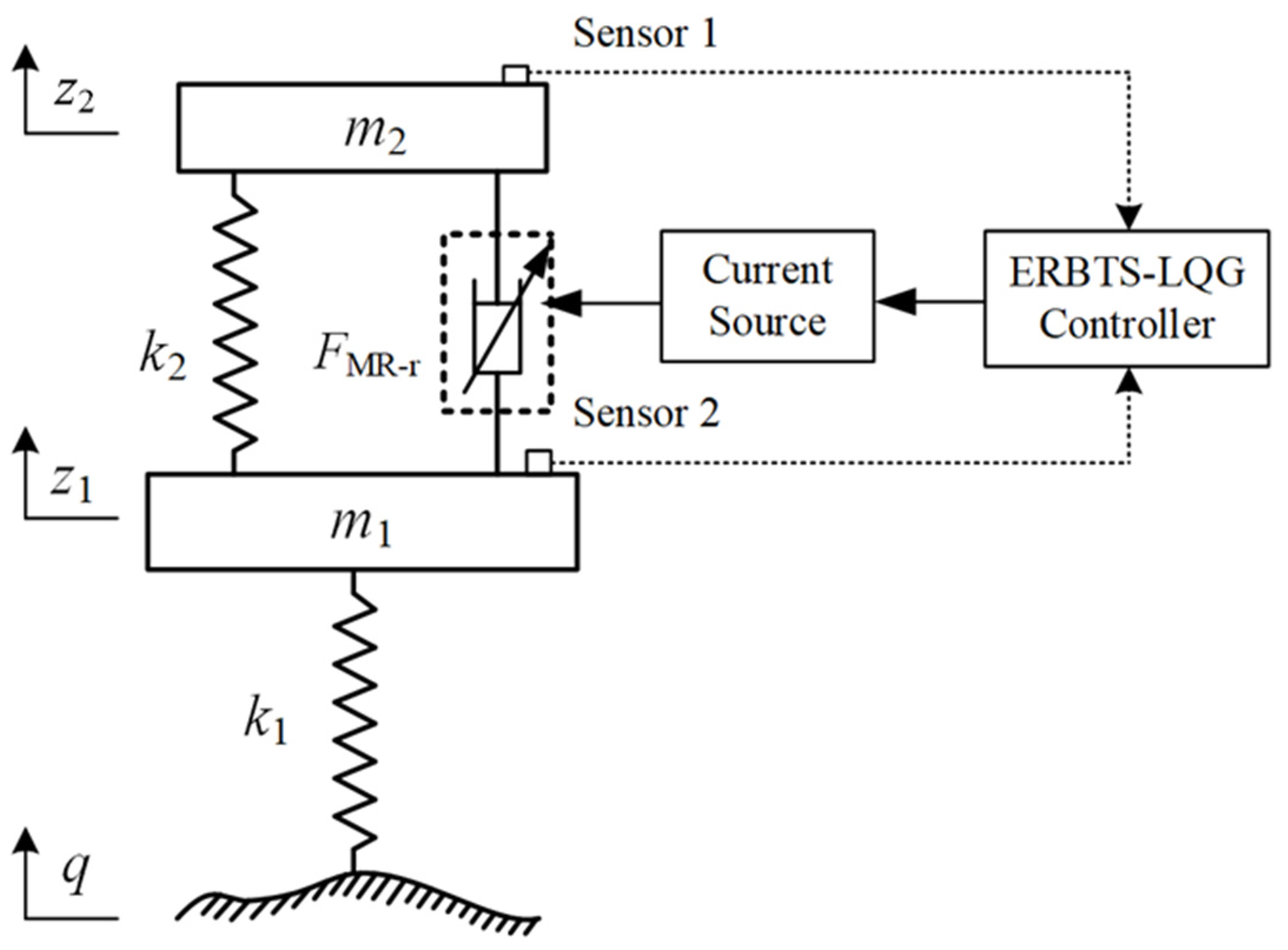
The rest of this paper is organized as follows: Section 2 addresses the nonlinear model of the MR semi-active suspension system. In Section 3, the ERBTS-LQG control scheme is presented. Section 4 provides a superiority verification of the proposed control scheme. Finally, the research is concluded in Section 5.

2. Model of the MR Semi-Active Suspension System

2.1. Vehicle Vertical Motion Model

A quarter-vehicle plant is adopted in Figure 1 to describe the MR semi-active suspension system.

A quarter-vehicle plant is adopted in Figure 1 to describe the MR semi-active suspension system.

$$\left\{\begin{array}{l}{m}_1{\ddot{z}}_1+k_1\left(z_1-q\right)+k_2\left(z_1-z_2\right)=-F_{\mathrm{MR}\_\mathrm{r}}\\ m_2{\ddot{z}}_2+k_2\left(z_2-z_1\right)=F_{\mathrm{MR}\_\mathrm{r}}\end{array}\right.$$

(1)

where $m_1$ and $m_2$ are the unsprung mass and the sprung mass, respectively; $k_1$ and $k_2$ stand for the tire stiffness and the suspension stiffness, respectively; $z_1$ and $z_2$ are the unsprung mass displacement and the sprung mass displacement, respectively; $F_{\mathrm{MR}\_\mathrm{r}}$ denotes the real-time output force of the MR damper; and $q$ is the displacement input from road roughness, expressed as follows [16]:

$$\left\{\begin{array}{l}\dot{q}(t)=-2\pi f_{0}q(t)+2\pi n_0\sqrt{0.5G_{\mathrm{q}}\left(n_0\right)u}w(t)\hfill \\ \mathsf{\Delta }s={\left(2u{n}_{\max }\right)}^{-1}\hfill \end{array}\right.$$

(2)

where $n_0$ is the reference spatial frequency of 0.1 m⁻¹; w indicates the road white-noise signal; $G_{\mathrm{q}}\left(n_0\right)$ is the road irregularity coefficient under the reference spatial frequency; u is the vehicle running speed; $f_0$ is the lower cutoff frequency of road input; $n_{\max }$ represents the higher cutoff frequency of road input; and $\mathsf{\Delta }s$ is the set value of sampling interval of the road white-noise signal.

Compared with other typical parametric models, the magic formula model has the inherent advantage of good parameter consistency, which is widely used for modelling MR dampers [17,18]. When the asymptotic saturation magic formula model is adopted, $F_{\mathrm{MR}\_\mathrm{r}}$ is presented as follows:

$$F_{\mathrm{MR}\_\mathrm{r}}=\mathsf{\Delta }F+F_{\mathrm{MR}}+F_{\mathrm{de}}$$

(3)

where $\mathsf{\Delta }F$ is the real-time variety relative to the nominal output force; $F_{\mathrm{de}}$ depicts the modelled error of the MR damper; $F_{\mathrm{MR}}$ depicts the nominal output force of the MR damper and is usually obtained by bench test, which can be expressed as follows:

$$F_{\mathrm{MR}}=D\tanh \left\{C\tanh \left[B\left(1-E\right)v+\frac{E}{B}\tanh \left(Bv\right)+F\tanh \left(Ma\right)\right]\right\}+c_{\mathrm{d}}v+k_{\mathrm{d}}\left(z_2-z_1\right)+F_{\mathrm{d}0}$$

(4)

where $B$, $C$, $D$, $E$, $F$, and $M$ are the stiffness factor, shape factor, peak factor, curvature factor, hysteresis width factor, and inertia factor, respectively; $v$ and $a$ represent the velocity and acceleration of the asymptotic saturation magic formula, respectively; $c_{\mathrm{d}}$ and $k_{\mathrm{d}}$ are the viscous and stiffness coefficients, respectively; $F_{\mathrm{d}0}$ stands for the basal force of the MR damper in bench test.

Compared with other fitting parameters, the peak factor fluctuation of the asymptotic saturation magic formula $D$ is most related to the change in the exciting current at different frequencies. To improve the fitting accuracy of the model, the expression of $D$ can be rewritten in a nonlinear expression:

$$D=D_0+D_{1}I+D_2{I}^2$$

(5)

where $D_0$, $D_1$, and $D_2$ represent the constant, primary, and secondary term coefficients, respectively; $I$ represents the exciting current.

By substituting Equation (5) in Equation (4), the equation can be rewritten as follows:

$$F_{\mathrm{MR}}=F_{\mathrm{MR}\_\mathrm{I}}\left(t-\tau \right)+F_{\mathrm{MR}\_0}+c_{\mathrm{d}}v+k_{\mathrm{d}}\left(z_2-z_1\right)+F_{\mathrm{d}0}$$

(6)

$$F_{\mathrm{MR}\_\mathrm{I}}=(D_{1}I+D_2{I}^2)\tanh \left\{C\tanh \left[B\left(1-E\right)v+\frac{E}{B}\tanh \left(Bv\right)+F\tanh \left(Ma\right)\right]\right\}$$

$$F_{\mathrm{MR}\_0}=D_0\tanh \left\{C\tanh \left[B\left(1-E\right)v+\frac{E}{B}\tanh \left(Bv\right)+F\tanh \left(Ma\right)\right]\right\}$$

where $F_{\mathrm{MR}\_\mathrm{I}}$ denotes the MR damper output force controlled by the current; t is the time variable; $\tau$ refers to the response delay time of the MR damper; $F_{\mathrm{MR}\_0}$ stands for the uncontrolled output force.

2.2. Actual Measurement-Based Parameter Identification

A bench test of the MR damper is implemented to identify model parameters, which is depicted in Figure 2.

The experimental bench of the MR damper mechanical characteristics measurement mainly consists of a single-channel hydraulic servo excitation console, a force transducer (DYLY-103), a current source (Zhaoxin KXN-3020D), and an NI data acquisition card. A commercially available MR damper (Type: BWI-23111781; from China, Beijing West Industries International Limited) is applied to conduct the damping force characteristics tests, whose maximum output force and maximum bilateral stroke approximately equal 3.5 kN and 22 cm, respectively. The experimental temperature is chosen as 60 °C, and the displacement inputs are 0.05 m-amplitude sine waves with exciting frequencies from 0.5 Hz to 2 Hz with increments of 0.5 Hz, and the control currents are from 0.5 A to 3 A with increments of 0.5 A.

Based on the Lsqcurvefit tool of MATLAB (R2013A) software, the unknown parameters of Equations (3)–(6) are fitted under different test conditions (each condition with different frequencies and exciting currents). The fitting principle of the Lsqcurvefit tool is set based on the least variance algorithm, expressed as follows:

$$\min {‖F_{\mathrm{MR}}^{\prime }-{\hat{F}}_{\mathrm{MR}}‖}_2^2=\min {\displaystyle \sum {\left[F_{\mathrm{MR}}^{\prime }-{\hat{F}}_{\mathrm{MR}}\right]}^2}$$

(7)

where $F_{\mathrm{MR}}^{\prime }$ and ${\hat{F}}_{\mathrm{MR}}$ represent the fitting output force and the actual output force measured during the mechanical characteristic test, respectively.

The identified results are listed in

Table 1. Identified parameter results of the MR damper model.

Parameter	Value	Parameter	Value
D0	0.1702	E	19.7348
D1	0.9304	F	−1.0860
D2	−0.0068	M	0.5955
C	0.4116	$k_{\mathrm{d}}$/kN	0.6854
B	−0.3092	$c_{\mathrm{d}}$	0.7696
$F_{\mathrm{d}0}$/kN	0.6908

.

The comparisons between the modelled and experimental curves under 0.5 Hz and 2 Hz are presented in Figure 3 and Figure 4. The solid lines represent the experimental curves marked by “T-XX A”, and the dashed lines refer to the modelled curves marked by “M-XX A”.

Figure 3 and Figure 4 indicate that there is an offset force (including the gravity of the exciting head, the gravity of the fixture, and the pressure required to compress the piston rod into the middle position) in the measured output force, which leads to a reduction in the measured output force range. The value of the offset force is approximately 0.6105 kN. Moreover, when the exciting frequency is set as 0.5 Hz, the error percentages between the experimental and optimized parameters are 6.29%, 5.21%, 5.11%, 4.35%, 5.88%, and 6.45%, respectively, and the control currents are from 0.5 A to 3 A with increments of 0.5 A. Furthermore, when the exciting frequency is set as 2 Hz, the error percentages are 7.43%, 6.26%, 5.09%, 4.96%, 5.77%, and 7.12%, respectively, under the same corresponding control currents.

Although there are still some inevitable errors, the applied asymptotic saturation magic formula model closely matches the experimental results. When the following augmented Kalman estimator is adopted, those inevitable modelling errors can be taken as one part of the real-time variation in the MR damper output force. Hence, one of the advantages of the proposed augmented Kalman estimator method is not having to construct a complex and accurate mechanical model of the MR damper.

2.3. Time Delay Measurement of MR Damper

Measuring the MR damper response time is the basis of time delay compensation control. Therefore, a rapid response current source driving the MR damper is designed, as depicted in Figure 5. The current source adopts a topology composed of two symmetrical N-channel MOS transistors and P-channel MOS transistors.

Figure 6 shows the demanded current, actual current, and output force of the MR damper under the testing condition with the sine displacement and square wave current inputs. The impact of offset force is removed through data processing in this figure.

It can be seen that, whatever the exciting displacement frequency, both the MR damper’s rising and descending response times (time delays) linearly increase with the control current. The sine displacement excitation has an amplitude of 50 mm and a frequency of 2.0 Hz. The square wave current excitation has an amplitude of 3.0 A and a frequency of 10 Hz. Figure 6 shows that, on the one hand, the rising and falling response times of the actual current equal 2.2 ms and 2.1 ms, respectively. The corresponding rising and falling response times of the output force are 9.0 ms and 7.9 ms, respectively. Considering that the rising response time is nearly equal to the falling response time, a mean of 8.5 ms is adopted as the response time of the MR damper output force in the following research. On the other hand, at this point, the current output force is equal to 2.267 kN, which does not exceed the maximum amplitude of 2.6 kN measured in Figure 4 for the MR damper. Due to some systematic errors (such as the variation of the current controlling the magneto-rheological fluid and the properties of the fluid itself), there are visible fluctuations in the MR damper force.

2.4. Control Objective

The suspension comprehensive performance index $J$ is expressed as follows [19]:

$$J=\underset{T\to \infty }{\lim }\frac{1}{T}{\displaystyle {\int }_0^T\left[{\ddot{z}}_2^2+{\delta }_1{\left(z_1-q\right)}^2+{\delta }_2{\left(z_2-z_1\right)}^2\right]}\mathrm{d}t$$

(8)

where δ₁ and δ₂ are the weights of ${\left(z_1-q\right)}^2$ and ${\left(z_2-z_1\right)}^2$, respectively, when the weight of ${\ddot{z}}_2^2$ is set as 1. A smaller J means better suspension comprehensive performance.

When the MR damper is installed on board, $F_{\mathrm{d}0}$ shall be offset by the suspension static deflection, and substituting Equations (3)–(6) into Equation (1) yields

$$\left\{\begin{array}{l}{m}_1{\ddot{z}}_1+k_1\left(z_1-q\right)+\left(k_2+k_{\mathrm{d}}\right)\left(z_1-z_2\right)+c_{\mathrm{d}}\left({\dot{z}}_1-{\dot{z}}_2\right)\hfill \\ =-\mathsf{\Delta }F-F_{{\mathrm{MR}}_{-}0}-F_{\mathrm{MR}\_\mathrm{I}}(t-\tau )-F_{\mathrm{de}}\hfill \\ m_2{\ddot{z}}_2+\left(k_2+k_{\mathrm{d}}\right)\left(z_2-z_1\right)+c_{\mathrm{d}}\left({\dot{z}}_2-{\dot{z}}_1\right)\hfill \\ =\mathsf{\Delta }F+F_{{\mathrm{MR}}_{-}0}+F_{\mathrm{MR}\_\mathrm{I}}(t-\tau )+F_{\mathrm{de}}\hfill \end{array}\right.$$

(9)

When the state vector $X={\left(x_1,x_2,x_3,x_4\right)}^{\mathrm{T}}$, it is defined as follows:

$$x_1=z_1-q,x_2=z_2-z_1,x_3={\dot{z}}_1,x_4={\dot{z}}_2$$

(10)

$$\stackrel{.}{X}=AX+BU+GW$$

(11)

$$A=\left[\begin{array}{cccc}0& 0& 1& 0\\ 0& 0& -1& 1\\ -\frac{k_1}{m_1}& \frac{k_2+k_{\mathrm{d}}}{m_1}& -\frac{c_{\mathrm{d}}}{m_1}& \frac{c_{\mathrm{d}}}{m_1}\\ 0& -\frac{k_2+k_{\mathrm{d}}}{m_2}& \frac{c_{\mathrm{d}}}{m_2}& -\frac{c_{\mathrm{d}}}{m_2}\end{array}\right],$$

$$B={\left[\begin{array}{cccc}0& 0& -\frac{1}{m_1}& \frac{1}{m_2}\end{array}\right]}^{\mathrm{T}}, G={\left[\begin{array}{cccc}-1& 0& 0& 0\end{array}\right]}^{\mathrm{T}},$$

$$U=\left[\mathsf{\Delta }F+F_{\mathrm{MR}\_0}+F_{\mathrm{MR}\_\mathrm{I}}\left(t-\tau \right)+F_{\mathrm{de}}\right], W=\left[\dot{q}\right]$$

3. Scheme for Time Delay Compensation Control

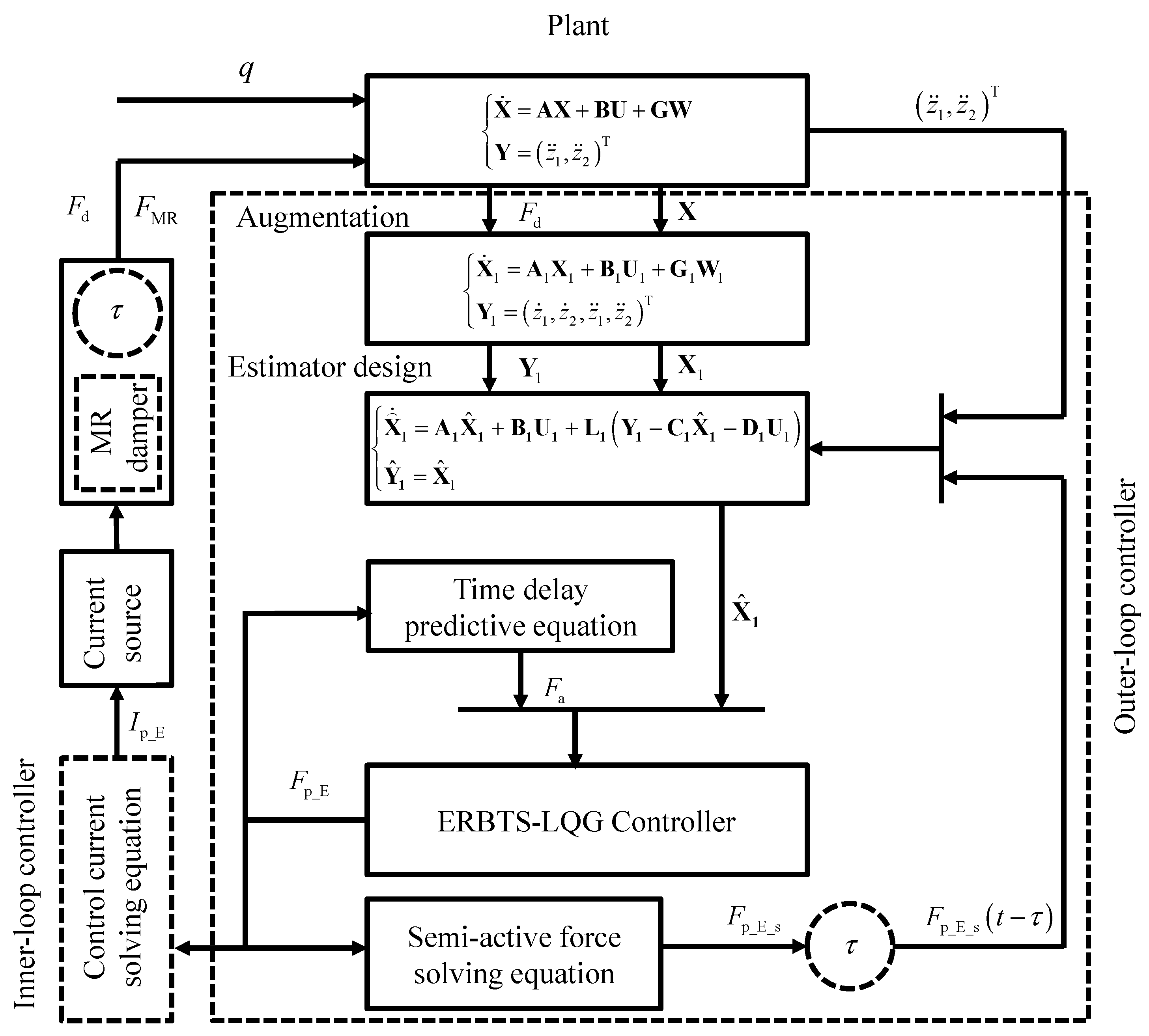
The scheme of the augmented Kalman estimator and the ERBTS-LQG controller is illustrated in Figure 7.

The proposed scheme involves three key steps.

(1)

The system state equation is augmented by the differential equation of the compound time variation of the MR damper output force.

(2)

The corresponding augmented Kalman estimator is designed to observe the system state vector and the compound real-time variety.

(3)

The ERBTS-LQG controller is developed by replacing a part of the squared time delay control force in the suspension comprehensive performance index with the corresponding predictive control force.

3.1. Design of the Augmented Kalman Estimator

For the sake of convenience, write $\mathsf{\Delta }F+F_{\mathrm{de}}$ as follows:

$$F_{\mathrm{d}}=\mathsf{\Delta }F+F_{\mathrm{de}}$$

(12)

Here, we name $F_{\mathrm{d}}$ the compound real-time variety of the MR damper output force.

To ensure the augmented system state equation with the characteristic of the minimum system, $F_{\mathrm{d}}$ is written in the differential equation as follows [19]:

$${\dot{F}}_{\mathrm{d}}=-\lambda F_{\mathrm{d}}+q_{\mathrm{d}},\hspace{0.33em}\hspace{0.33em}\hspace{0.33em}\lambda >0$$

(13)

where $q_{\mathrm{d}}$ is the related parameters of $F_{\mathrm{d}}$, and $\lambda$ indicates the positive infinitely small quantity.

Substituting Equations (12) and (13) into Equation (11) yields the augmented system state equation as follows:

$${\dot{X}}_1=A_1{X}_1+B_1{U}_1+G_1{W}_1$$

(14)

$$X_1=\left[\begin{array}{l}X\hfill \\ F_d\hfill \end{array}\right],A_1=\left[\begin{array}{cc}A& B\\ 0_{1\times 4}& -\lambda \end{array}\right],B_1=\left[\begin{array}{c}B\\ 0\end{array}\right],G_1=\left[\begin{array}{cc}G& 0_{4\times 1}\\ 0& 1\end{array}\right]$$

$$U_1=\left[F_{\mathrm{MR}\_\mathrm{I}}\left(t-\tau \right)+F_{\mathrm{MR}\_0}\right],W_1=\left[\begin{array}{l}\dot{q}\\ q_d\end{array}\right].$$

Considering that the acceleration is easy to detect, and ${\ddot{z}}_2$ are chosen as the outputs of the MR semi-active suspension system. In this work, to improve observation accuracy, integrals of the two accelerations are chosen as the inputs of the augmented Kalman estimator.

The corresponding output equation is expressed as

$$Y_1={\left[\begin{array}{cccc}{\dot{z}}_1& {\dot{z}}_2& {\ddot{z}}_1& {\ddot{z}}_2\end{array}\right]}^{\mathrm{T}}=C_1{X}_1+D_1{U}_1$$

(15)

$$C_1=\left[\begin{array}{c}\left[\begin{array}{ccccc}0& 0& 1& 0& 0\end{array}\right]\\ \left[\begin{array}{ccccc}0& 0& 0& 1& 0\end{array}\right]\\ A_1(3,:)\\ A_1(4,:)\end{array}\right],D_1={\left[\begin{array}{cccc}{0}_{1\times 1}& 0_{1\times 1}& B_1(3,1)& B_1(4,1)\end{array}\right]}^{\mathrm{T}}$$

The augmented Kalman estimator is designed as follows:

$$\left\{\begin{array}{l}{\stackrel{.}{\hat{X}}}_1=A_1{\hat{X}}_1+B_1{U}_1+L_1\left(Y_1-C_1{\hat{X}}_l-D_1{U}_1\right)\hfill \\ {\hat{Y}}_1={\hat{X}}_1\hfill \end{array}\right.$$

(16)

$$L_1=\left(P_{\mathrm{K}}{C}_1^{\mathrm{T}}+G_1{N}_{\mathrm{K}}\right)R_{\mathrm{K}}^{-1}$$

(17)

where ${\hat{X}}_1$ stands for the estimate of $X_1$; $P_{\mathrm{K}}$ represents the unique solution of the following Riccati equation.

$$\begin{array}{l}{A}_1{P}_{\mathrm{K}}+P_{\mathrm{K}}{\mathrm{A}}_1^{\mathrm{T}}-\left(P_{\mathrm{K}}{C}_1^{\mathrm{T}}+G_1{N}_{\mathrm{K}}\right)R_{\mathrm{K}}^{-1}\left(C_1{P}_{\mathrm{K}}+N_{\mathrm{K}}^{\mathrm{T}}{G}_1^{\mathrm{T}}\right)\\ +G_1{Q}_{\mathrm{K}}{G}_1^{\mathrm{T}}=0\end{array}$$

(18)

$$\left\{\begin{array}{l}{Q}_{\mathrm{K}}=\mathrm{E}\left\{W_1^{\mathrm{T}}{W}_1\right\}\hfill \\ R_{\mathrm{K}}=\mathrm{E}\left\{V_1^{\mathrm{T}}{V}_1\right\}\hfill \\ N_{\mathrm{K}}=\mathrm{E}\left\{W_1^{\mathrm{T}}{V}_1\right\}\hfill \end{array}\right.$$

(19)

where $V_1$ is the measurement noise vector.

Therefore, using the newly developed Kalman estimator, in addition to the system state vector $X$, the compound real-time variety of the MR damper output force $F_{\mathrm{d}}$ is estimated.

3.2. Design of the ERBTS-LQG Controller

Usually, $F_{{\mathrm{MR}}_{-}\mathrm{I}}(t-\tau )$ is expressed as

$$\left\{\begin{array}{l}{F}_{{\mathrm{MR}}_{-}\mathrm{I}}(t-\tau )=\left\{\begin{array}{ll}{F}_{\mathrm{a}}(t-\tau )\hfill & \mathrm{when} \hspace{0.33em}\hspace{0.33em}\hspace{0.33em}{v}_{\mathrm{e}}\left[F_{\mathrm{a}}(t-\tau )+D_0{v}_{\mathrm{e}}\right]<0\hfill \\ -D_0{v}_{\mathrm{e}}\hfill & \mathrm{else} \hfill \end{array}\right.\hfill \\ v_{\mathrm{e}}=\tanh \left\{C\tanh \left[\begin{array}{l}B(1-E)\left({\dot{z}}_2-{\dot{z}}_1\right)\hfill \\ +\frac{E}{B}\tanh B\left({\dot{z}}_2-{\dot{z}}_1\right)+F\tanh M\left({\ddot{z}}_2-{\ddot{z}}_1\right)\hfill \end{array}\right]\right\}\hfill \end{array}\right.$$

(20)

where $F_{\mathrm{a}}$ refers to the active control force.

To obtain better suspension performance, the constant time delay of the MR damper must be considered in the controller sign. When the Taylor series-LQG strategy is applied, the active predictive control force $F_{\mathrm{p}}$ and the corresponding $F_{\mathrm{MR}\_\mathrm{I}\_\mathrm{p}}$ are expressed as follows:

$$F_{\mathrm{p}}=F_{\mathrm{a}}(t+\tau )\approx F_{\mathrm{a}}+\tau {\dot{F}}_{\mathrm{a}}$$

(21)

$$F_{\mathrm{MR}\_\mathrm{I}\_\mathrm{p}}\left(t-\tau \right)=\left\{\begin{array}{l} F_{\mathrm{p}}\left(t-\tau \right)=F_{\mathrm{a}}\\ \mathrm{when}\begin{array}{c}\end{array}{v}_{\mathrm{e}}\left[F_{\mathrm{p}}\left(t-\tau \right)+D_0{v}_{\mathrm{e}}\right]<0\\ -D_{0}v\\ \mathrm{else}\end{array}\right.$$

(22)

Substituting Equation (21) into Equation (14) yields the state equation as follows:

$${\stackrel{.}{X}}_2=A_2{X}_2+B_2{U}_{2\mathrm{a}}+G_2{W}_2$$

(23)

$$X_2=\left[\begin{array}{l}{\hat{X}}_1\hfill \\ F_{\mathrm{a}}\hfill \end{array}\right],A_2=\left[\begin{array}{cc}{A}_1& B_1\\ 0_{1\times 5}& -\frac{1}{\tau }\end{array}\right],B_2=\left[\begin{array}{c}{0}_{5\times 1}\\ \frac{1}{\tau }\end{array}\right],$$

$$G_2=\left[\begin{array}{c}{G}_1\\ 0_{1\times 2}\end{array}\right],U_{2\mathrm{a}}=\left[F_{\mathrm{p}}\right],\cdot W_2=W_1.$$

On the basis of $X_2$, $U_{2\mathrm{a}}$, and Equation (10), the cost function of the ideal time delay compensation system is written as

$$J_{\mathrm{a}}=\underset{T\to \infty }{\lim }\frac{1}{T}{\displaystyle {\int }_0^{\mathrm{T}}\left[X_2^{\mathrm{T}}Q{X}_2+2X_2^{\mathrm{T}}N{U}_{2\mathrm{a}}+U_{2\mathrm{a}}^{\mathrm{T}}R{U}_{2\mathrm{a}}\right]}\mathrm{d}t$$

(24)

$$\begin{array}{ll}\hfill Q=& {\delta }_1{\left[\begin{array}{llllll}1\hfill & 0\hfill & 0\hfill & 0\hfill & 0\hfill & 0\hfill \end{array}\right]}^{\mathrm{T}}\left[\begin{array}{llllll}1\hfill & 0\hfill & 0\hfill & 0\hfill & 0\hfill & 0\hfill \end{array}\right] \hfill \\ & +{\delta }_2{\left[\begin{array}{llllll}0\hfill & 1\hfill & 0\hfill & 0\hfill & 0\hfill & 0\hfill \end{array}\right]}^{\mathrm{T}}\left[\begin{array}{llllll}0\hfill & 1\hfill & 0\hfill & 0\hfill & 0\hfill & 0\hfill \end{array}\right]\hfill \\ & +A_2{(4,:)}^{\mathrm{T}}{A}_2(4,:),\hfill \end{array}$$

$$N=A_2{(4,:)}^{\mathrm{T}}{B}_2(4,:)=0_{6\times 1},$$

$$R=B_2{(4,:)}^{\mathrm{T}}{B}_2(4,:)=0_{1\times 1}.$$

In Equation (24), $R=0$ does not satisfy the second LQG controller design condition that $R>0$.

To solve the abovementioned problem, the approximate transformation can be expressed as follows:

$$\left\{\begin{array}{l}{F}_{\mathrm{p}}(t-\tau )=\alpha F_{\mathrm{p}}(t-\tau )+\beta F_{\mathrm{p}}(t)\hfill \\ \alpha +\beta =1\hfill \\ \alpha >>>0\hfill \end{array}\right.$$

(25)

Although $R=0$ is avoided, that method will give an overly large value of $F_{\mathrm{p}}$. This factor could be due to the following two reasons. The first is that, by using Equation (25), the control objective becomes inaccurate. The other is that Equation (25) brings a considerably small R that cannot effectively constrain $F_{\mathrm{p}}$.

To obtain a better time delay compensation control effect, Corollary 1 is proposed to effectively constrain the predictive control force to precisely track the control objective $J_{\mathrm{a}}$.

Corollary 1. 

when sufficiently large, positive $\gamma$ satisfies

$$Q_{2\mathrm{E}}=Q_2-\left[\begin{array}{cc}{0}_{5\times 5}& 0_{5\times 1}\\ 0_{1\times 5}& \gamma \end{array}\right]\ge 0$$

(26)

and the following active force$F_{{\mathrm{p}}_{-}\mathrm{E}}$precisely tracks the control objective $J_{\mathrm{a}}$.

$$F_{{\mathrm{p}}_{-}\mathrm{E}}=-K_{{\mathrm{p}}_{-}\mathrm{E}}{X}_2$$

(27)

$$K_{\mathrm{p}\_\mathrm{E}}=R_{2\mathrm{E}}^{-1}\left(B_2^{\mathrm{T}}{S}_{{\mathrm{p}}_{-}\mathrm{E}}+N_2^{\mathrm{T}}\right)$$

(28)

$$R_{2\mathrm{E}}=[\gamma ]$$

(29)

where $S_{{\mathrm{p}}_{-}\mathrm{E}}$is the unique solution of the Riccati equation as follows:

$$A_2^{\mathrm{T}}{S}_{{\mathrm{p}}_{-}\mathrm{E}}+S_{{\mathrm{p}}_{-}\mathrm{E}}{A}_2-\left(S_{{\mathrm{p}}_{-}\mathrm{E}}{B}_2+N_2\right)R_{2\mathrm{E}}^{-1}\left(B_2^{\mathrm{T}}{S}_{{\mathrm{p}}_{-}\mathrm{E}}+N_2^{\mathrm{T}}\right)+Q_{2\mathrm{E}}=0$$

(30)

Proof. 

Implementing the Fourier transform on $F_{\mathrm{p}\_\mathrm{E}}(t-\tau )$ yields

$$\begin{array}{c}\mathcal{F}\left[F_{\mathrm{p}\_\mathrm{E}}\left(t-\tau \right)\right]={\displaystyle {\int }_{-\infty }^{\infty }{F}_{\mathrm{p}\_\mathrm{E}}}\left(t-\tau \right)e^{-\mathrm{j}\omega t}\mathrm{d}t={\displaystyle {\int }_{-\infty }^{\infty }{F}_{\mathrm{p}\_\mathrm{E}}\left(t\right)}{e}^{-\mathrm{j}\omega \left(t+\tau \right)}\mathrm{d}t\\ =e^{-\mathrm{j}\omega \tau }{\displaystyle {\int }_{-\infty }^{\infty }{F}_{\mathrm{p}\_\mathrm{E}}}\left(t\right)e^{-\mathrm{j}\omega t}\mathrm{d}t=e^{-\mathrm{j}\omega \tau }\mathcal{F}\left[F_{\mathrm{p}\_\mathrm{E}}\left(t\right)\right],\end{array}$$

(31)

where $\mathrm{j}=\sqrt{-1}$ and $\omega$ is the circular frequency. □

Then, the 2-norm value of $\mathcal{F}\left[F_{\mathrm{p}\_\mathrm{E}}\left(t-\tau \right)\right]$ can be written as follows:

$${‖\mathcal{F}\left[F_{\mathrm{p}\_\mathrm{E}}\left(t-\tau \right)\right]‖}_2={‖\mathcal{F}\left[F_{\mathrm{p}\_\mathrm{E}}\left(t\right)\right]‖}_2{‖e^{-\mathrm{j}\omega \tau }‖}_2={‖\mathcal{F}\left[F_{\mathrm{p}\_\mathrm{E}}\left(t\right)\right]‖}_2.$$

(32)

Writing Equation (32) into the time domain form yields

$$\underset{T\to \infty }{\lim }{\displaystyle {\int }_0^T{F}_{{\mathrm{p}}_{-}\mathrm{E}}^2}(t-\tau )\mathrm{d}t=\underset{T\to \infty }{\lim }{\displaystyle {\int }_0^T{F}_{{\mathrm{p}}_{-}\mathrm{E}}^2}(t)\mathrm{d}t$$

(33)

According to Equations (21) and (33), the following equation can be obtained.

$$\underset{T\to \infty }{\lim }{\displaystyle {\int }_0^T{F}_{{\mathrm{p}}_{-}\mathrm{E}}^2}\mathrm{d}t=\underset{T\to \infty }{\lim }{\displaystyle {\int }_0^T{F}_a^2}\mathrm{d}t$$

(34)

Thus,

$$\begin{array}{l}\underset{T\to \infty }{\lim }\frac{1}{T}{\displaystyle {\int }_0^T\left[X_2^{\mathrm{T}}{Q}_{2\mathrm{E}}{X}_2+2X_2^{\mathrm{T}}{N}_2{U}_{2\mathrm{E}}+{U_{2\mathrm{E}}}^{\mathrm{T}}{R}_{2\mathrm{E}}{U}_{2\mathrm{E}}\right]}\mathrm{d}t\\ =\underset{T\to \infty }{\lim }\frac{1}{T}{\displaystyle {\int }_0^T\left[{\left(\begin{array}{c}{X}_1\\ F_{\mathrm{i}}\end{array}\right)}^{\mathrm{T}}\left[Q_2-\left[\begin{array}{cc}{0}_{5\times 5}& 0_{5\times 1}\\ 0_{1\times 5}& \gamma \end{array}\right]\right]\left(\begin{array}{c}{X}_1\\ F_{\mathrm{i}}\end{array}\right)+{\left(F_{\mathrm{p}\_\mathrm{E}}\right)}^{\mathrm{T}}\left[\gamma \right]\left(F_{\mathrm{p}\_\mathrm{E}}\right)\right]}\mathrm{d}t\\ =\underset{T\to \infty }{\lim }\frac{1}{T}{\displaystyle {\int }_0^T\left[X_2^{\mathrm{T}}{Q}_2{X}_2\right]}\mathrm{d}t-\underset{T\to \infty }{\lim }{\displaystyle {\int }_0^T\gamma F_{\mathrm{i}}^2}\mathrm{d}t+\underset{T\to \infty }{\lim }{\displaystyle {\int }_0^T\gamma F_{\mathrm{p}\_\mathrm{E}}^2}\mathrm{d}t\\ =\underset{T\to \infty }{\lim }\frac{1}{T}{\displaystyle {\int }_0^T\left[X_2^{\mathrm{T}}{Q}_2{X}_2\right]}\mathrm{d}t=J_{\mathrm{a}}\end{array}$$

(35)

Hence, all the design conditions of the LQG controller are satisfied, and $F_{\mathrm{p}\_\mathrm{E}}$ precisely tracks $J_{\mathrm{a}}$. The proof is completed.

By using Equations (26), (29) and (34), a part of the squared time delay control force in the suspension comprehensive performance index is equivalently replaced by the corresponding part of the predictive control force. Because this replacement is completely equivalent, this novel time delay compensation control method is called the equivalent replacement-based Taylor series-LQG control approach. It should be noted that the above operation is proposed first in this work and is difficult to realize by using the ${\mathrm{H}}_2$ control method.

Therefore, the corresponding semi-active predictive control force $F_{{\mathrm{p}}_{-}{\mathrm{E}}_{-}\mathrm{s}}$ is as follows:

$$F_{{\mathrm{p}}_{-}{\mathrm{E}}_{-}\mathrm{s}}=\left\{\begin{array}{ll}{F}_{{\mathrm{p}}_{-}\mathrm{E}}\hfill & \mathrm{when} v_{\mathrm{e}}\left[F_{{\mathrm{p}}_{-}\mathrm{E}}(t-\tau )+D_0{v}_{\mathrm{e}}\right]<0\hfill \\ -D_0{v}_{\mathrm{e}}\hfill & \mathrm{else} \hfill \end{array}\right.$$

(36)

Because $\left|D_1\right|\gg \left|D_2\right|$, the predictive control current $I_{{\mathrm{p}}_{-}\mathrm{E}}$ is calculated as follows:

$$I_{{\mathrm{p}}_{-}\mathrm{E}}=\left\{\begin{array}{l}{I}_{\max }\hfill \\ \mathrm{when} v_{\mathrm{e}}{F}_{{\mathrm{p}}_{-}{\mathrm{E}}_{-}\mathrm{s}}<0 \mathrm{and} \frac{-F_{{\mathrm{p}}_{-}{\mathrm{E}}_{-}\mathrm{s}}}{\mathrm{sign}\left(v_{\mathrm{e}}\right)\left(\left|v_{\mathrm{e}}\right|+0.001\right)}<I_{\max }\hfill \\ \frac{-F_{{\mathrm{p}}_{-}{\mathrm{E}}_{-}\mathrm{s}}}{\mathrm{sign}\left(v_{\mathrm{e}}\right)\left(\left|v_{\mathrm{e}}\right|+0.001\right)}\hfill \\ \mathrm{when} v_{\mathrm{e}}{F}_{{\mathrm{p}}_{-}{\mathrm{E}}_{-}\mathrm{s}}<0 \mathrm{and} \frac{-F_{{\mathrm{p}}_{-}{\mathrm{E}}_{\mathrm{s}}}}{\mathrm{sign}\left(v_{\mathrm{e}}\right)\left(\left|v_{\mathrm{e}}\right|+0.001\right)}\le I_{\max }\hfill \\ 0\hspace{0.33em}\hspace{0.33em}\hspace{0.33em} \mathrm{else} \hfill \end{array}\right.$$

(37)

where $I_{\max }$ is the maximum control current to the MR damper.

In Equation (37), by replacing $v_{\mathrm{e}}$ with $\mathrm{sign}\left(v_{\mathrm{e}}\right)\left(\left|v_{\mathrm{e}}\right|+0.001\right)$, we can avoid the issue of $I_{{\mathrm{p}}_{-}\mathrm{E}}$ not being calculated when $v_{\mathrm{e}}=0$.

4. Superiority Verifications

From the point of view of vehicle weight and operating conditions, the abovementioned MR semi-active suspension system can be fitted on sport or utility vehicles.

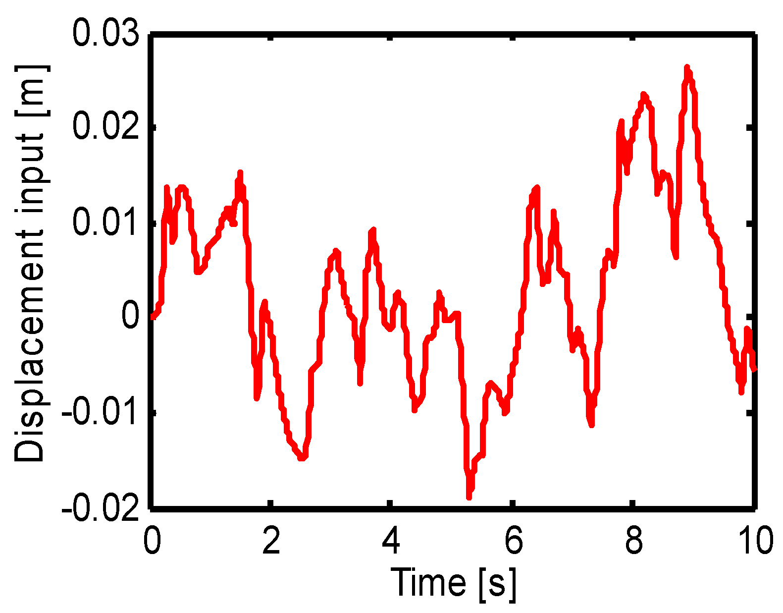
The driving condition of v = 50 m·s⁻¹ over the D-class road (D-cr) is investigated, which corresponds to a poorly constructed road with a relatively low velocity [20]. Under the v = 50 km/h over the D-class road, the value of $G_{\mathrm{q}}\left(n_0\right)$ presented in Equation (2) is set as 1024 × 10⁻⁶ m⁻¹. From Equation (2), we can obtain the displacement input curve in Figure 8.

The other vehicle parameters are listed in

Table 2. Parameters needed in research.

Parameters	Values	Parameters	Values
$m_1$ [kg]	36	$k_2$ [N/m]	50,000
$m_2$ [kg]	520	$u$ [km/h]	50
$k_1$ [N/m]	270,000	${\delta }_1$	37,888
${\delta }_2$	4660.1

.

4.1. Observation Accuracy of the Augmented Kalman Estimator

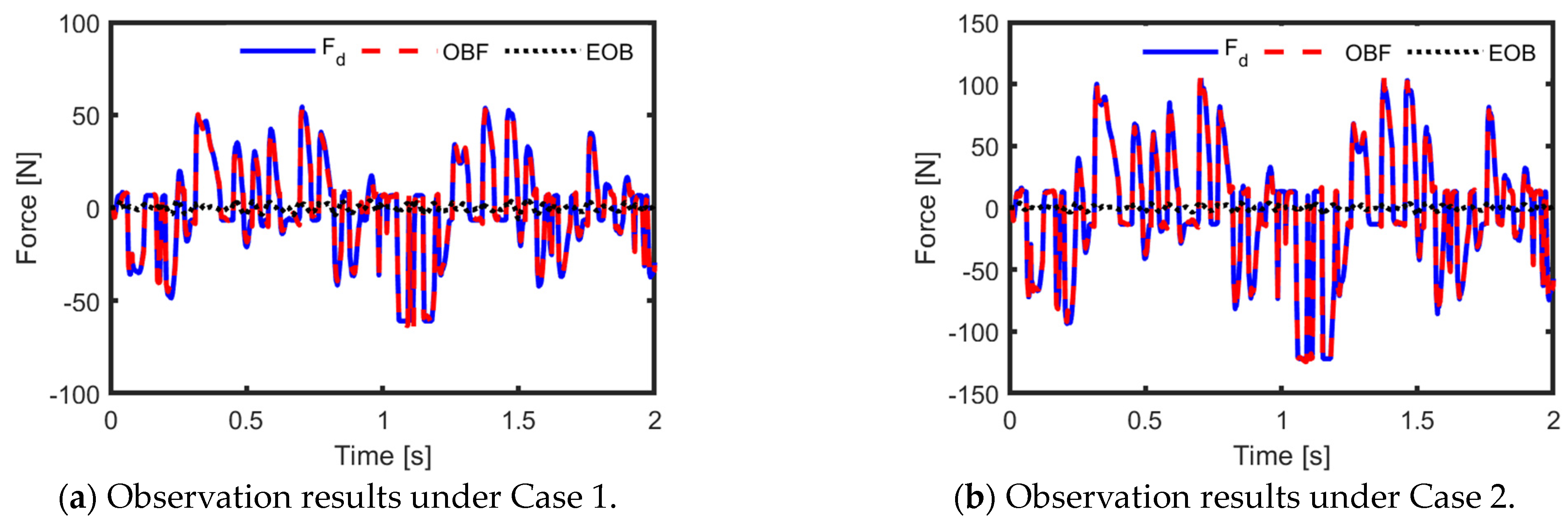
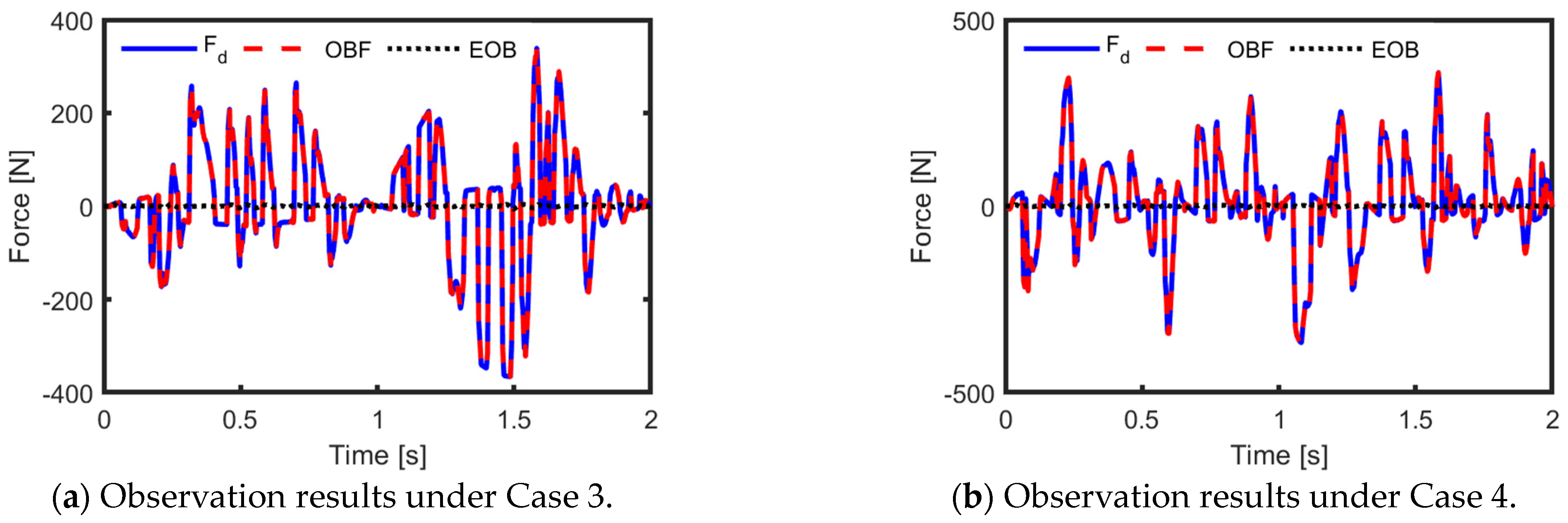
To clearly display the work effectiveness of the augmented Kalman estimator, four cases are checked:

Case 1: A small modelling error with $F_{\mathrm{d}}=0.05\times \left(F_{\mathrm{MR}\_0}+F_{\mathrm{p}\_\mathrm{E}\_\mathrm{s}}\right)$;

Case 2: A large modelling error with $F_{\mathrm{d}}=0.1\times \left(F_{\mathrm{MR}\_0}+F_{\mathrm{p}\_\mathrm{E}\_\mathrm{s}}\right)$;

Case 3: A considerably large real-time variety with $F_{\mathrm{d}}=0.3\sin \left(\mathsf{\pi }t\right)\times \left(F_{\mathrm{MR}\_0}+F_{\mathrm{p}\_\mathrm{E}\_\mathrm{s}}\right)$;

Case 4: A considerably large and fast real-time variety with $F_{\mathrm{d}}=0.3\sin \left(6\mathsf{\pi }t\right)\times \left(F_{\mathrm{MR}\_0}+F_{\mathrm{p}\_\mathrm{E}\_\mathrm{s}}\right)$.

The observation error and the corresponding root mean square (RMS) error are defined as follows:

$${\mathrm{E}}_{\mathrm{ob}}=F_{\mathrm{d}}-{\hat{F}}_{\mathrm{d}}$$

(38)

$$\mathrm{RMSE}=\frac{\mathrm{RMS}\left(F_{\mathrm{d}}-{\hat{F}}_{\mathrm{d}}\right)}{\mathrm{RMS}\left(F_{\mathrm{d}}\right)}$$

(39)

where ${\hat{F}}_{\mathrm{d}}$ is the observation of $F_{\mathrm{d}}$ and $\mathrm{RMS}()$ denotes the function calculating the root mean square.

The observation effectiveness of the augmented Kalman estimator is described in Figure 9 and Figure 10. In these figures, “OBF” and “EOB” stand for the observation of $F_{\mathrm{d}}$ and the observation error, respectively.

The observation errors, the RMSEs, and the corresponding suspension comprehensive performance indexes of those five cases are listed in

Table 3. Parameters needed in research.

	RMS (${\mathbf{E}}_{\mathbf{ob}}$)	RMSE	J
Case 1	1.7134	0.0549	5.2127
Case 2	1.7047	0.0280	5.2129
Case 3	1.7631	0.0126	5.2472
Case 4	1.7590	0.0130	5.2296

.

Figure 9 and Figure 10 show that all ${\hat{F}}_{\mathrm{d}}$ curves track the $F_{\mathrm{d}}$ curves well under the above investigation cases. Moreover, Table 3 shows that the root mean square of ${\mathrm{E}}_{\mathrm{ob}}$ is at almost the same level of less than 2. When a modelling error of 5% exists, the worst observation accuracy occurs, and the RMSE equals 0.0549. Compared with the integral of $F_{\mathrm{p}\_\mathrm{E}\_\mathrm{s}}$, the RMSE is just 0.0027. This is a very high observation accuracy. Even though there are 10% modelling errors and 30% real-time variations, compared with the integral of $F_{\mathrm{p}\_\mathrm{E}\_\mathrm{s}}$, the RMSE is just 0.0031. In addition, subjected to those investigation cases, the maximum difference in the suspension comprehensive performance index is equal to 0.0048.

The above investigation results demonstrate that the augmented Kalman estimator is a perfect solution for both the modelling error and real-time variety of the MR damper output force.

4.2. Work Effectiveness of the ERBTS-LQG Controller

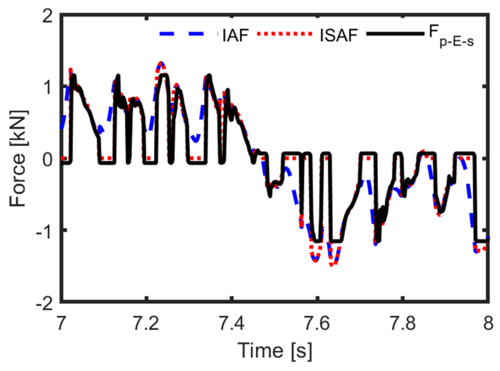
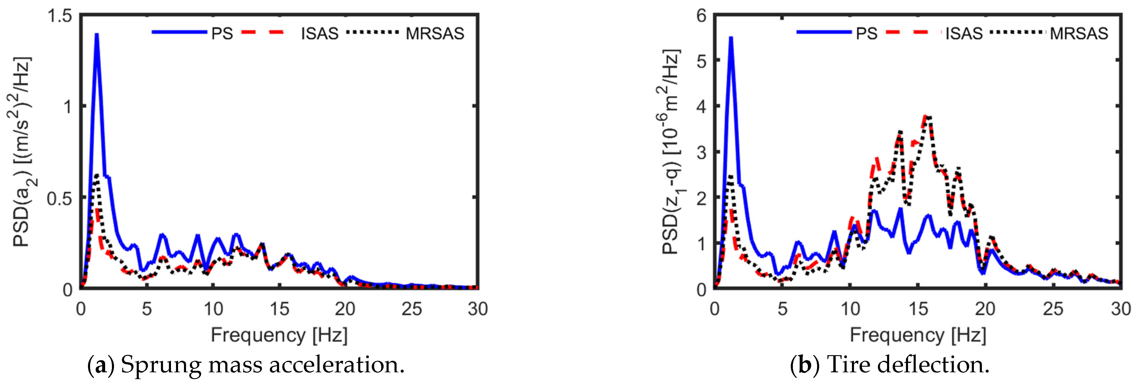
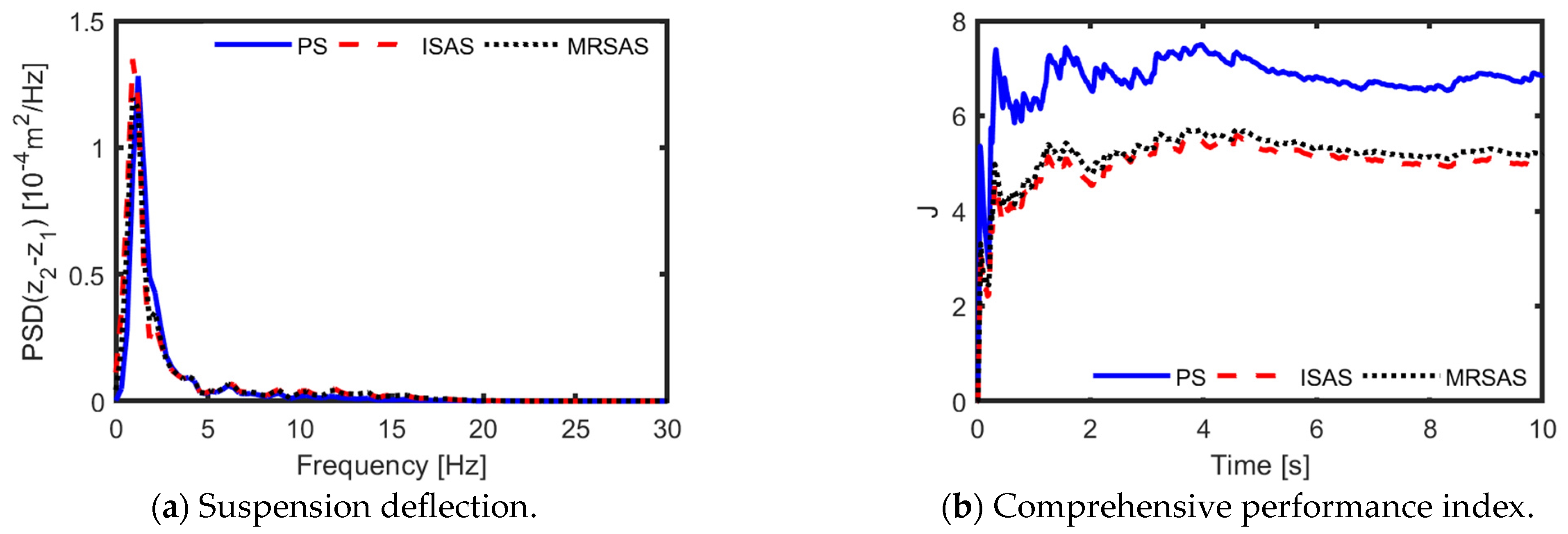
It is assumed that the MR semi-active suspension suffers from both modelling error and real-time variety. To verify the superiority of the ERBTS-LQG controller, the sprung mass acceleration, the tire deflection, the suspension deflection, and the suspension comprehensive performance index are compared among the passive suspension, the time delay free semi-active suspension, and the MR semi-active suspension regulated by the proposed time delay compensation controller. These three suspensions are denoted by “PS”, “ISAS”, and “MRSAS”. The ideal active force (IAF), the ideal semi-active force (ISAF), and $F_{\mathrm{p}\_\mathrm{E}\_\mathrm{s}}$ curves in the time domain are illustrated in Figure 11. The comparison curves of the suspension performances in the frequency domain are drawn in Figure 12 and Figure 13.

At the turning point when the ideal semi-active force is in need or disappears, Figure 11 illustrates that $F_{\mathrm{p}\_\mathrm{E}\_\mathrm{s}}$ and the ideal semi-active force are almost synchronous. This means that after a time delay, the predictive semi-active force can accurately track the ideal semi-active force. Additionally, $F_{\mathrm{p}\_\mathrm{E}\_\mathrm{s}}$ is less than the ideal semi-active force. The reason can be explained as follows: the actual MR damper output force is constrained by the maximum control current of 3 A.

Figure 12 and Figure 13 clearly illustrate that both the tire deflection and the suspension deflection of the MR semi-active suspension are almost the same as those of the ideal suspension. Moreover, compared with the passive suspension, the proposed ERBTS-LQG controller regulates the MR semi-active suspension to obviously reduce the suspension comprehensive performance index and the peak value of the PSD of the unsprung mass acceleration. Moreover, the PSD of tire deflection for ISAS and MRSAS are worse compared to the PS in the frequency range from 10 to 20 Hz. This is because the driving condition of v = 50 m·s⁻¹ over the ISO D-class road (D-cr) is regarded as a low-velocity driving condition. In this condition, the riding comfort is usually given priority. To obtain a better riding comfort, a larger weight coefficient of sprung mass acceleration is selected, which results in unsatisfactory improvement of tire deflection. This result is reasonable. The RMSs of those suspension performance indicators are listed in

Table 4. Statistical data of the four suspension performance indicators.

Indicator	PS	ISAS	MRSAS
RMS(a2) [m/s2]	2.2210	1.6732	1.7510
RMS(z1 − q) [m]	0.0053	0.0057	0.0056
RMS(z2 − z1) [m]	0.0136	0.0146	0.0142
J	6.8525	5.0350	5.2089

.

In this table, compared with the passive suspension, the MR semi-active suspension and the ideal semi-active suspension decrease the unsprung mass acceleration by 21.16% and 24.66%, respectively. For the suspension comprehensive performance index, the corresponding decreases are 23.99% and 26.52%, respectively.

Figure 12 and Figure 13 and Table 4 show that the unsprung mass acceleration and the suspension comprehensive performance index of the ideal semi-active suspension are just slightly better than those of the MR semi-active suspension using the proposed ERBTS-LQG controller. The reason can be explained as follows. First, by using Equation (21), there is a system error in calculating the active predictive control force. Moreover, when an active force with negative damping characteristics is needed, unlike the ideal semi-active suspension, which can be given a control force equal to zero, the MR semi-active suspension inevitably suffers from an uncontrolled positive damping output force.

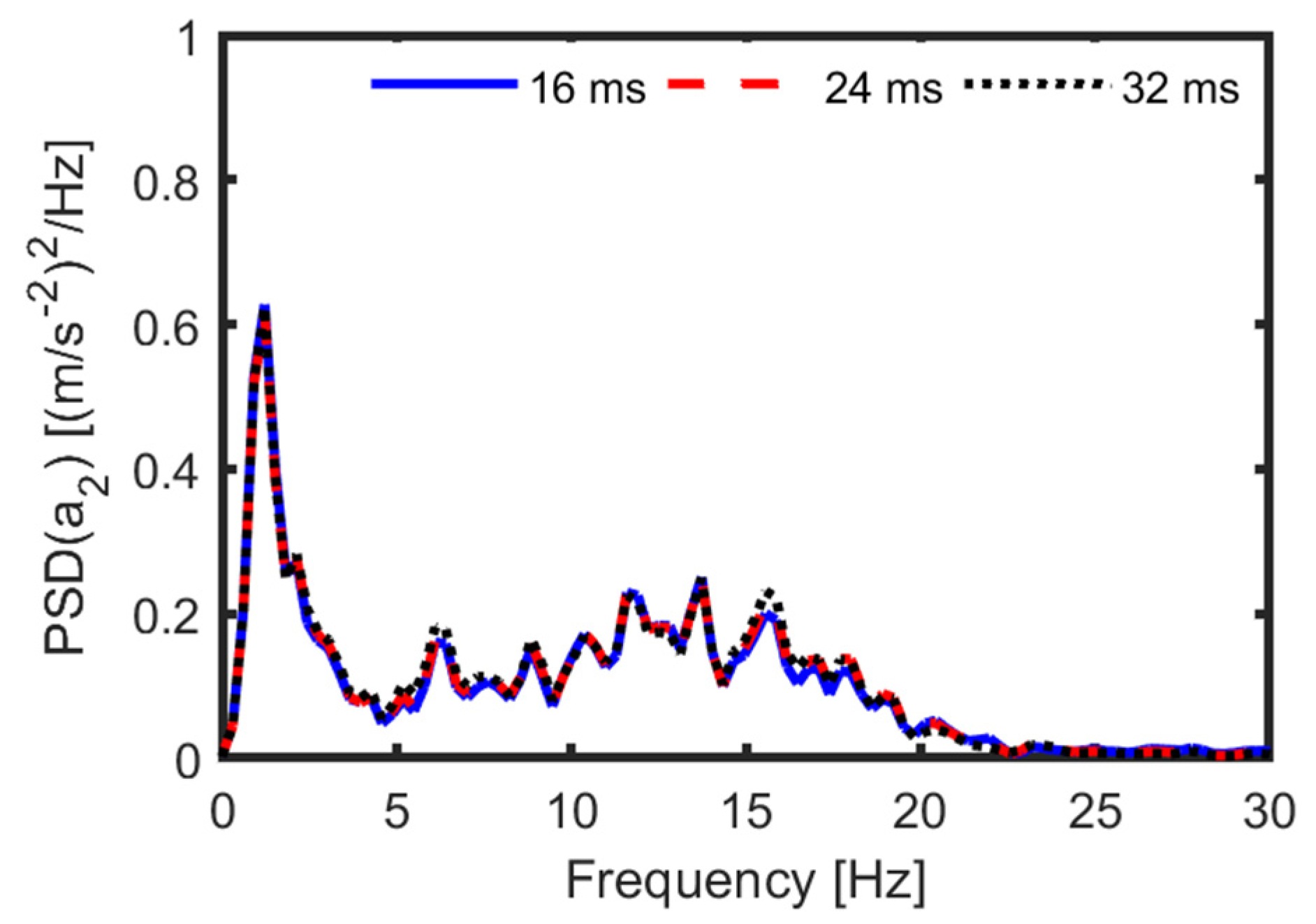
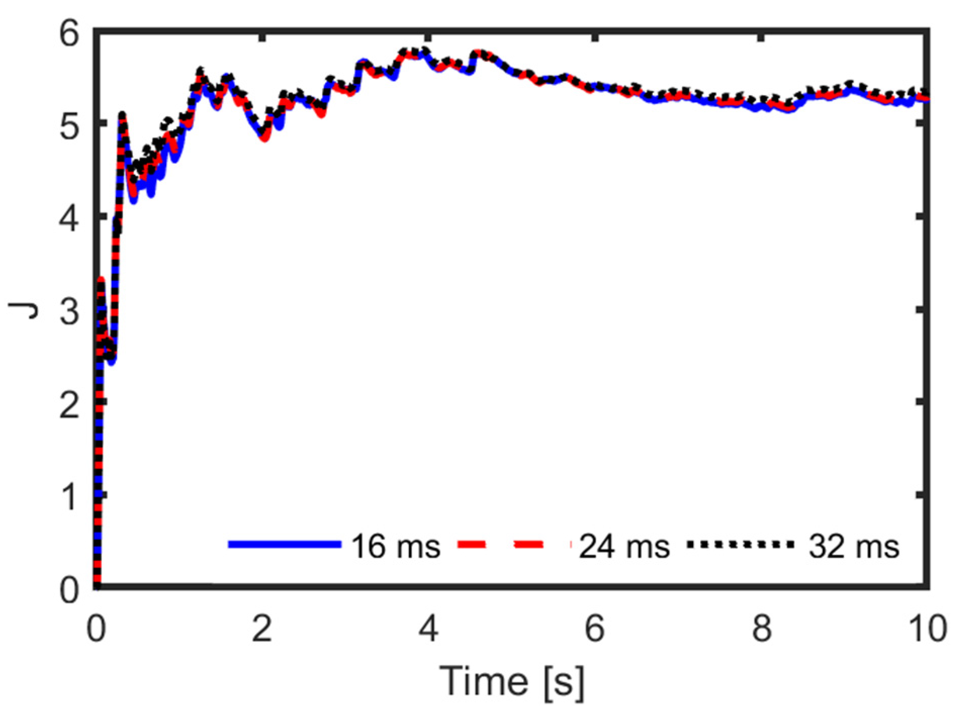
To check the adaptability of the proposed ERBTS-LQG controller, some other large time delay cases are investigated. These cases refer to time delays equal to 16 ms, 24 ms, and 32 ms. Comparison curves of the unsprung mass acceleration and the suspension comprehensive performance index are depicted in Figure 14 and Figure 15, respectively. Statistical data of the four suspension performance indicators are provided in

Table 5. Statistical data of the four suspension performance indicators.

Indicators	16 ms	24 ms	32 ms
RMS(a2) [m/s2]	1.7673	1.7831	1.8037
RMS(z1 − q) [m]	0.0056	0.0056	0.0056
RMS(z2 − z1) [m]	0.0142	0.0140	0.0138
J	5.2613	5.2850	5.3384

.

Figure 14 shows that when the time delay changes from 16 ms to 32 ms, the PSD of the unsprung mass acceleration only slightly increases around the natural frequency of wheel vibration. Similarly, Figure 15 clearly illustrates that the suspension comprehensive performance index only slightly degrades. It can be seen in Table 4 and Table 5 that when the time delay increases from 8.5 ms to 16 ms, 24 ms, and 32 ms, the RMS of the unsprung mass acceleration is enlarged by 0.93%, 1.83%, and 3.01%, respectively. The corresponding increases in the suspension comprehensive performance index are 1.01%, 1.46%, and 2.49%, respectively.

The above results indicate that when subjected to a time delay from 8.5 ms to 32 ms, the ERBTS-LQG controller always regulates the MR semi-active suspension to achieve very near control effectiveness of the ideal time delay-free semi-active suspension. In particular, the proposed controller has excellent time delay compensation ability and adaptability.

5. Conclusions

A novel augmented Kalman estimator and ERBTS-LQG controller are developed to cope with the modelling error and large time delay of MR dampers for vehicle semi-active suspension. The main conclusions are summarized as follows:

(1)

The augmented Kalman estimator is established to observe the compound real-time variety of the MR damper output force by expressing it as a differential equation with the characteristic of the minimum system to augment the state space equation of the semi-active suspension system.

(2)

The equivalent replacement-based Taylor series-LQG controller is newly developed to improve the effect of time delay compensation by replacing a part of the squared time delay control force in the suspension comprehensive performance index with the corresponding predictive control force.

References

1. Luo, J.W.; Li, P.S.; Li, P.X.; Cai, Q.Q. Observer-based multi-objective integrated control for vehicle lateral stability and active suspension design. J. Sound Vib. 2021, 508, 25. [Google Scholar] [CrossRef]
2. Issa, M.; Samn, A. Passive vehicle suspension system optimization using Harris Hawk Optimization algorithm. Math. Comput. Simul. 2022, 191, 328–345. [Google Scholar] [CrossRef]
3. Theunissen, J.; Sorniotti, A.; Gruber, P.; Fallah, S.; Ricco, M.; Kvasnica, M.; Dhaens, M. Regionless explicit model predictive control of active suspension systems with preview. IEEE Trans. Ind. Electron. 2019, 67, 4877–4888. [Google Scholar] [CrossRef]
4. Deng, X.; Dong, X.; Li, W.; Xi, J. A grey hysteresis model of magnetorheological damper. J. Intell. Mater. Syst. Struct. 2022, 33, 1423–1438. [Google Scholar] [CrossRef]
5. Elsaady, W.; Oyadiji, S.O.; Nasser, A. A review on multi-physics numerical modelling in different applications of magnetorheological fluids. J. Intell. Mater. Syst. Struct. 2020, 31, 1855–1897. [Google Scholar] [CrossRef]
6. Wu, X.; Zhou, B.; Huang, J.; Qiu, X. Switched anti-roll control design for hydraulically interconnected suspension system with time delay. Int. J. Veh. Des. 2019, 79, 143–167. [Google Scholar] [CrossRef]
7. Pei, G.; Yu, M.; Xu, Y.; Ma, C.; Lai, H.; Chen, F.; Lin, H. An improved PID controller for the compliant constant-force actuator based on BP neural network and smith predictor. Appl. Sci. 2021, 11, 2685. [Google Scholar] [CrossRef]
8. Yu, X.; Liu, X.; Wang, X.; Wang, X.; Wang, Y. Vibration control of improved LQG for wheel drive electric vehicle based on uncertain parameters. Proc. Inst. Mech. Eng. Part D J. Automob. Eng. 2021, 235, 2253–2264. [Google Scholar] [CrossRef]
9. Wang, G.; Chen, H.; Zhou, Z. Comfort-enhanced vibration control for delayed active suspensions using relaxed inequalities. J. Low Freq. Noise Vib. Act. Control 2019, 38, 647–663. [Google Scholar] [CrossRef]
10. Na, J.; Huang, Y.; Wu, X.; Su, S.-F.; Li, G. Adaptive finite-time fuzzy control of nonlinear active suspension systems with input delay. IEEE Trans. Cybern. 2019, 50, 2639–2650. [Google Scholar] [CrossRef] [PubMed]
11. Liu, W.; Chen, G.; Knoll, A. Matrix inequalities based robust model predictive control for vehicle considering model uncertainties, external disturbances, and time-varying delay. Front. Neurorobot. 2021, 14, 617293. [Google Scholar] [CrossRef] [PubMed]
12. Pang, H.; Zhang, X.; Yang, J.; Shang, Y. Adaptive backstepping-based control design for uncertain nonlinear active suspension system with input delay. Int. J. Robust Nonlinear Control 2019, 29, 5781–5800. [Google Scholar] [CrossRef]
13. Yan, G.; Fang, M.; Xu, J. Analysis and experiment of time-delayed optimal control for vehicle suspension system. J. Sound Vib. 2019, 446, 144–158. [Google Scholar] [CrossRef]
14. Dong, X.; Yu, M.; Guan, Z. Adaptive sliding mode fault-tolerant control for semi-active suspension using magnetorheological dampers. J. Intell. Mater. Syst. Struct. 2011, 22, 1653–1660. [Google Scholar] [CrossRef]
15. Bharathi Priya, C.; Gopalakrishnan, N. Experimental investigations of the effect of temperature on the characteristics of MR damper. In Proceedings of the Recent Advances in Structural Engineering, Volume 2: Select Proceedings of SEC 2016; Springer: Singapore, 2019; Volume 2, pp. 435–443. [Google Scholar]
16. Shi-an, C.; Jia-cheng, T.; Xu-dong, J.; Ya-xiong, W.; Ming, Y. Modeling method for non-stationary road irregularity based on modulated white noise and lookup table method. J. Traffic Transp. Eng. 2020, 20, 171–179. [Google Scholar]
17. Bui, Q.; Bai, X.; Nguyen, Q. Dynamic modeling of MR dampers based on quasi–static model and Magic Formula hysteresis multiplier. Eng. Struct. 2021, 245, 112855. [Google Scholar] [CrossRef]
18. Xue, B.; Du, Y.; Liu, Y.; Wang, Y.; Wei, Y. A mechanism-based magic formula model for hysteretic characteristics of magneto rheological damper. J. Vib. Eng. 2017, 30, 774–780. [Google Scholar]
19. Wang, J.; Lv, L.; Ren, J.; Chen, S. Time delay compensation using a Taylor series compound robust scheme for a semi-active suspension with magneto rheological damper. Asian J. Control 2021, 24, 2632–2648. [Google Scholar] [CrossRef]
20. Kisilowski, J.; Zalewski, J. Modeling of Road Traffic Events, Springer: Berlin/Heidelberg, Germany, 2022.
Figure 1. Quarter vehicle model with the MR semi-active suspension system.
Actuators 13 00138 g001
Figure 2. Experimental bench of MR damper mechanical characteristics.
Actuators 13 00138 g002
Figure 3. Comparisons of modelled and experimental results under 0.5 Hz.
Actuators 13 00138 g003aActuators 13 00138 g003b
Figure 4. Comparisons of modelled and experimental results under 2.0 Hz.
Actuators 13 00138 g004
Figure 5. Working principle of the rapid response current source.
Actuators 13 00138 g005
Figure 6. Rising and falling response time curves of current and output force.
Actuators 13 00138 g006
Figure 7. Scheme of the augmented Kalman estimator and ERBTS-LQG controller.
Actuators 13 00138 g007
Figure 8. Displacement input under the ISO D-class road.
Actuators 13 00138 g008
Figure 9. Partial view of observation effectiveness under Cases 1 and 2.
Actuators 13 00138 g009
Figure 10. Partial view of observation effectiveness under Cases 3 and 4.
Actuators 13 00138 g010
Figure 11. Partial view of curves for IAF, ISAF, and F p _ E _ s in the time domain.
Actuators 13 00138 g011
Figure 12. Comparison curves of sprung mass acceleration and tire deflection.
Actuators 13 00138 g012
Figure 13. Comparison curves of suspension deflection and comprehensive performance index.
Actuators 13 00138 g013
Figure 14. Curves of sprung mass acceleration under different time delays.
Actuators 13 00138 g014
Figure 15. Curves of the suspension comprehensive performance index under different time delays.
Actuators 13 00138 g015