Terminal Sliding Mode Force Control Based on Modified Fast Double-Power Reaching Law for Aerospace Electro-Hydraulic Load Simulator of Large Loads

Abstract

This paper addresses the force-tracking problem of aerospace electro-hydraulic load simulators under the influence of high inertia, large loads, and a strong coupling force disturbance. An accurate mathematical model is initially derived to describe the characteristics of the load simulator system, the cause of the surplus force, and the strong phase lag due to large inertia. In order to overcome the position interference of the system and the large phase lag problem, a terminal sliding mode control strategy based on the modified fast double-power reaching law is proposed, based on the accurate mathematical model. This control strategy effectively suppresses the chattering problem of the sliding control and implements the finite time convergence of the system through the design of the reaching law and terminal sliding surface, ensuring the robustness of the system and the accuracy of the force-tracking problem. Finally, a comparison of the simulation and experimental results based on the design of different strategy controllers is performed to verify the effectiveness of the control strategy and system adaptability.

1. Introduction

The servo system, as a fundamental component of the launch vehicle control system, regulates the flight attitude of the rocket by controlling the deflection angles of the engine nozzles. Hence, the servo actuator must exhibit a rapid dynamic response and strong anti-interference capabilities during rocket operations. To address this requirement, a load simulation system is employed to replicate the diverse load characteristics of the high-power control objects of the servomechanism. This load simulation system provides load-testing conditions for dynamic variables that closely resemble real-world scenarios for research tests on the servomechanism, thereby playing a significant role in verifying servo control algorithms and evaluating the servomechanism’s performance.

The electro-hydraulic load simulator is a commonly used load simulation system, and it is a typical hardware-in-loop system [1], providing the actual experimental conditions for testing the system performance and the reliability of the servo actuator. Due to the mechanical coupling characteristics between the load system and the tested actuator, the active motion of the actuator results in an extra force on the loading side caused by forced flow, thus considerably affecting force-tracking precision and decreasing the stability of the system. Moreover, nonlinearities, mainly including flow pressure, friction and backlash characteristics, uncertainties caused by unstable parameters (i.e., the leakage coefficient, bulk modulus, and coefficient of viscosity), unknown disturbances, and sensor noises [2,3,4,5], critically degrade the precise force closed-loop control, dynamic performance, and static accuracy.

In order to mitigate the adverse impact of surplus force on the force loading and improve system performance, numerous scholars have extensively conducted research and experimentations with respect to both the mechanical structures and control algorithms. By manipulating the connection stiffness [6] and arm length [7] between the loading mechanism and the steering gear system, the connection mechanism is optimized in conjunction with a control algorithm, thus effectively mitigating the surplus force. The dual-valve parallel control that consists of the large flow valve and small servo valve is designed to achieve a high control accuracy in electro-hydraulic servo systems in [8]. To reduce the extra torque generated by the forced flow, substitution of the pressure servo valve for the flow servo valve is adopted in the passive force control system, to form a pressure closed-loop control for obtaining high-precision torque tracking in [9]. Overall, improving the mechanical structure leads to certain disadvantages like elevated cost, a limited capacity to mitigate surplus force, and constrained control. Therefore, sole dependance on this approach cannot effectively compensate for surplus force.

In terms of control strategy, a structure invariance compensation (SIC) control method, which utilizes the velocity feedback of the servo actuator as forward feedback compensation to isolate the driving torque from the driving speed, is proposed in [10] to compensate for the influence of interference from the tested servo actuator and suppress the surplus force. An active force control system is developed to provide an accurate real-time force loading for the landing gear of the M-346 “iron bird”, which is an integrated testing rig for the simulation, confirmation, and verification of the flight controls, hydraulic system, and landing gear of the M-346 trainer, adopting the servo valve to control the hydraulic actuator, combined with a nonlinear adaptive control law to achieve precise loading controls [11]. To account for the internal and external disturbances that affect the mechanism of the loading simulator, a more accurate mathematical model, including nonlinear factors and uncertainties, advanced control algorithms (i.e., backstepping [12], sliding mode, neural network [13], iterative learning control [14]), and sensor faults and disturbances observation [15,16], is utilized for accurate tracking and nonlinear compensation. The backstepping adaptive control, combined with the modified LuGre friction model [17], is introduced into the force-tracking control of the loading simulator [18]. This approach effectively weakens the distortion phenomenon caused by friction and results in a better force control performance. In a research study, a finite-time sliding mode control based on the modified GMS friction model, which is identified by PSO, has been designed to acquire an accurate system model and compensate for uncertain disturbances and nonlinear friction, ensuring the dynamic performance and static precision of the loading system, while achieving a finite-time convergence [19]. Parameter estimation [20,21] and identification [22], aimed at system uncertainties and nonlinear disturbances, integrated into a sliding force control model, is adopted to eliminate parametric uncertainties, which strengthens the system’s robustness, as well as exhibiting a strong anti-interference ability and loading accuracy. Based on a proposed disturbance coupled model containing mechanical backlash, a decoupled position interference and mitigated oscillation caused by the backlash are achieved by the control strategy of an almost disturbance decoupling. Moreover, the stability of the state and the system performance are ensured by tuning the controller parameters [23]. In general, numerous scholars have made significant contributions to the suppression of the surplus force of the load simulation system and the improvement of the corresponding control algorithms. They have achieved favorable results in their studies. However, the abovementioned control methods are generally aimed at medium and low loads with medium and low inertia, which are unsuitable for the load simulation systems with large loads and high inertia that are discussed in this paper.

The sliding mode control is particularly suitable for achieving a precise force closed-loop control in load simulation systems, due to its robustness, adaptability to nonlinear systems, and provable stability. It is a typical variable structure control, which has been researched widely and applied in nonlinear control strategies, owing to the characteristics of strong robustness and anti-interference ability, fast response, and simple physical implementation [24]. The chattering phenomenon and the complex finite convergence time are trending topics of research, which need to be resolved by scholars. A robust fixed-time sliding mode strategy has been designed, so that mismatched disturbances can be rejected without using a disturbance observer, and fixed-time stability can be obtained [25,26]. For obtaining dynamic response rapidity and convergence to the original in fixed time, the fast terminal sliding mode (TSM) has been designed by [27], where the nonlinear item is integrated to improve the approach rate and obtain finite-time convergence, while introducing a reaching rate that is lower than that of the linear sliding mode (LSM). Therefore, the global terminal sliding mode (FTSM) has been developed to combine the strengths of the FTSM and LSM, which ensures system rapidity and fixed-time reachability [28,29]. However, both the TSM and FTSM exhibit a critical challenge: singularity. A nonsingular terminal sliding mode control, utilized in wave energy converters, a miniature helicopter, and a robotic system [30,31,32], is proposed to address this issue, eliminating the singular item induced by the design of the controller and enhancing the engineering applicability. In [33], a fixed-time sliding control involving the cosine function is developed to simultaneously satisfy closed-loop system stability and the nonsingularity of the system. The small high-frequency oscillation in the vicinity of the sliding manifold, which is caused by the chattering phenomenon, hinders the application of the control strategy [34]. From an engineering perspective, K. D. Young et al. accurately analyze and evaluate the sliding mode control and its chattering phenomenon. Subsequently, they proposed seven solutions for mitigating the chattering effect in continuous systems and examined the design of the sliding mode control for discrete systems in three different scenarios, providing valuable guidance for the practical implementation of sliding mode controls [35]. The chattering at a high frequency is eliminated by the continuous switching of the boundary layer, due to the substitution of the signal function by the hyperbolic tangent function [36]. In [37], a sliding mode control based on the enhanced triple-power reaching law is proposed, to assure fixed-time convergence to the equilibrium point of the sliding surface in the system and eliminate chattering behaviors by means of the switchover of a set of prescribed switching manifolds. In this paper, an innovative approach is proposed for a load simulator of large inertia, which simultaneously addresses the finite-time convergence problem of both the reaching motion and the sliding motion of the sliding mode surface. The effectiveness of the approach is validated through simulation and experimentation, in conjunction with comparable control strategies.

Overall, the main contributions of this paper are as follows:

(1)

The causes and characteristics of surplus force and a significant phase lag are analyzed, based on a precise mathematical model derived from a high-inertia electro-hydraulic load simulator.

(2)

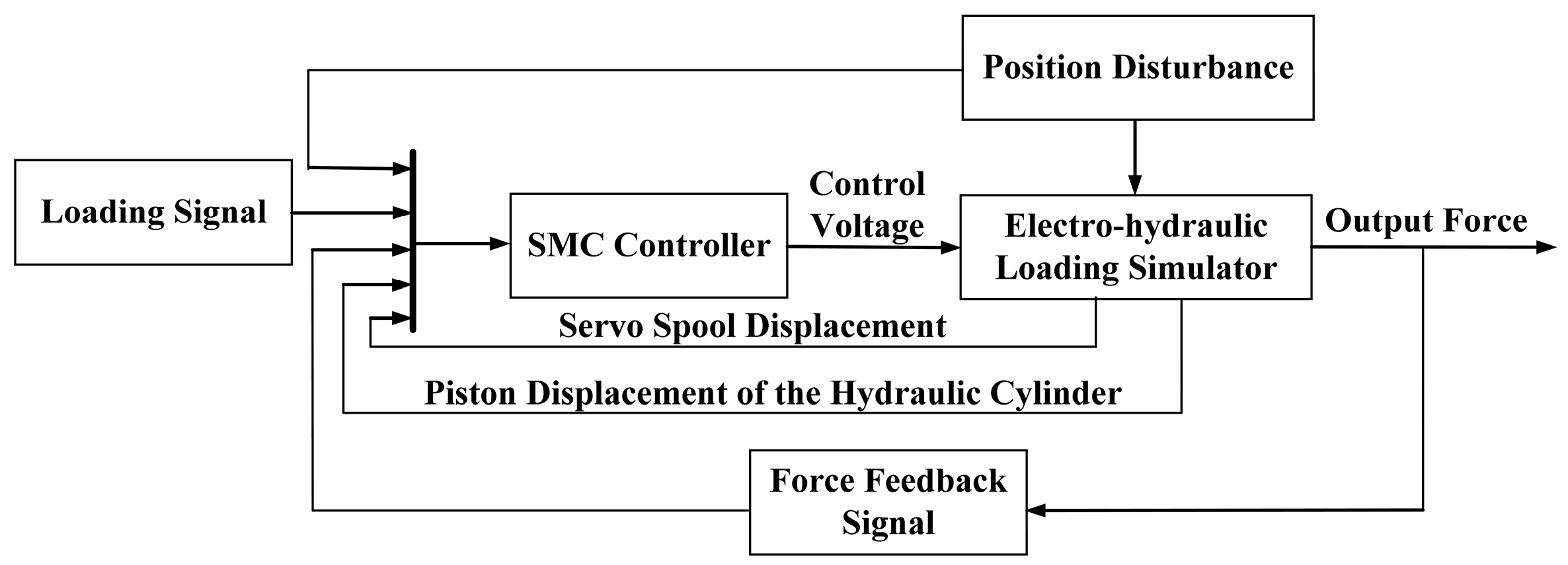
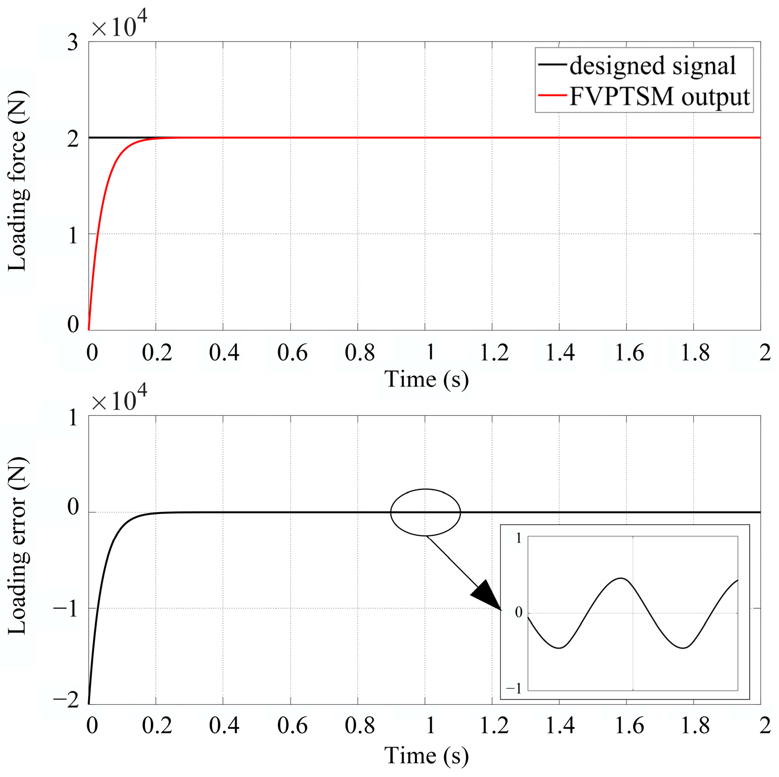
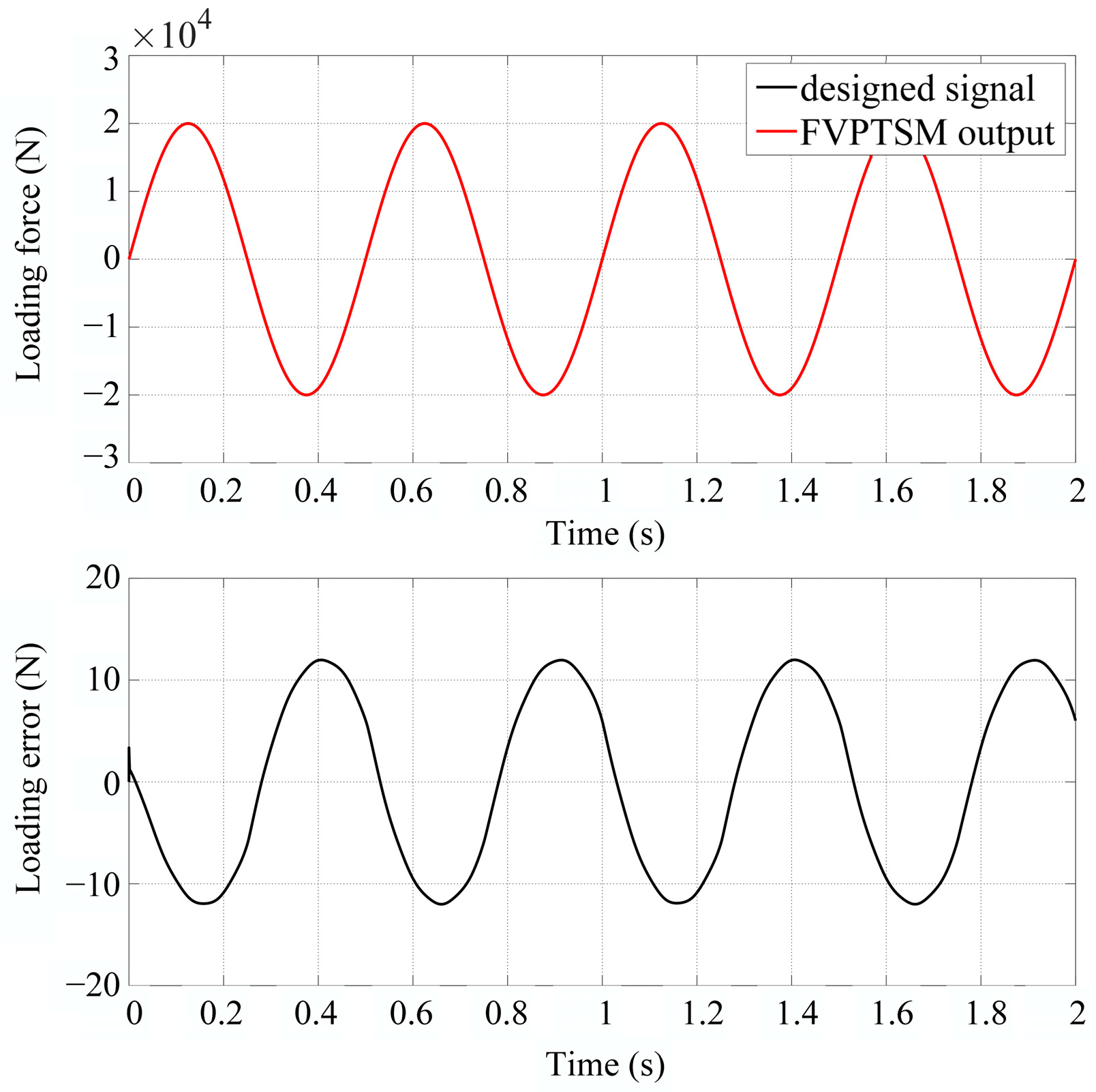
Aimed at a high-inertia electro-hydraulic load simulator, a modified fast variable-power terminal sliding mode control strategy (FVPTSM) is proposed, which achieves both a finite convergence time and a finite-time proof, while employing the Lyapunov theory for stability analysis.

(3)

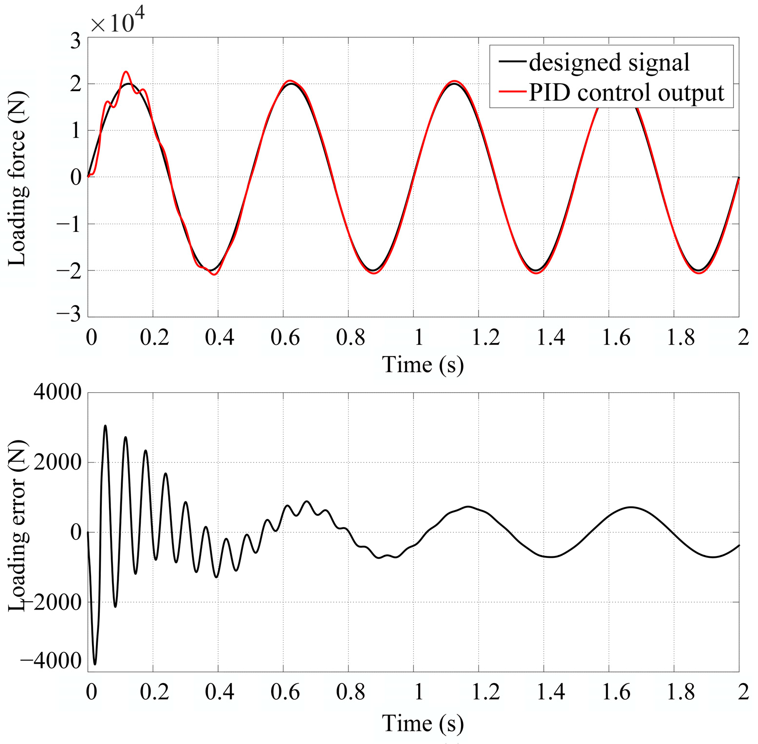
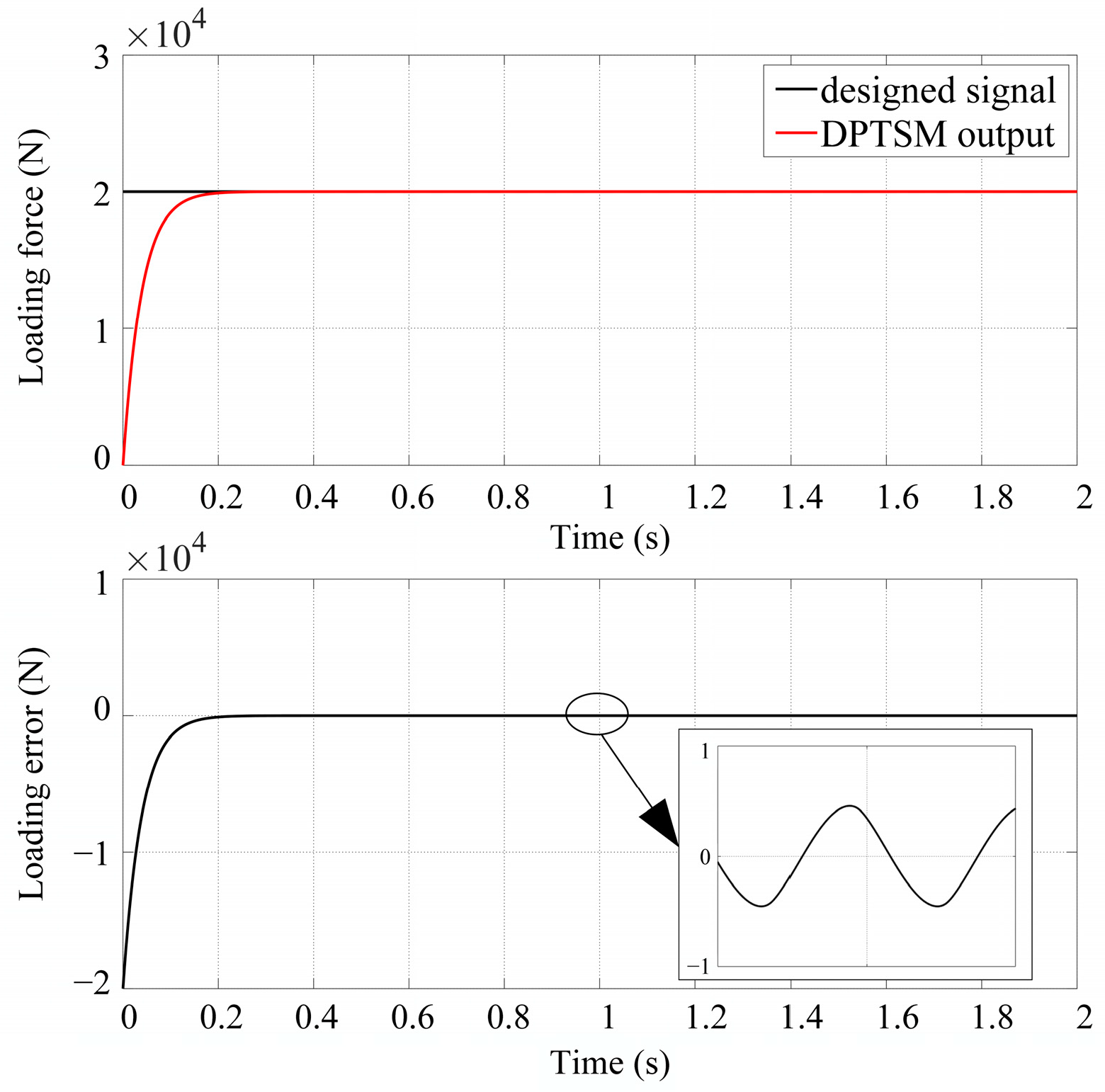
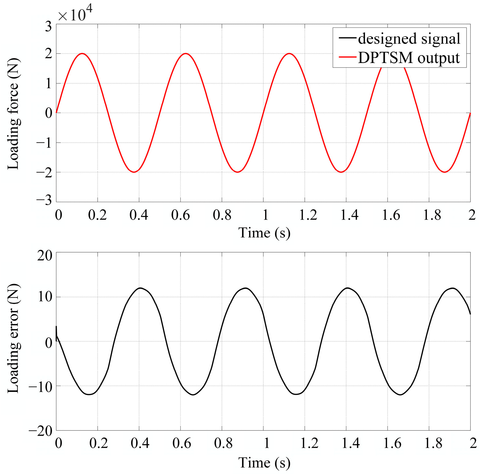
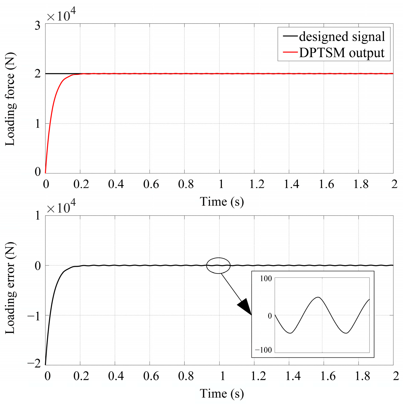
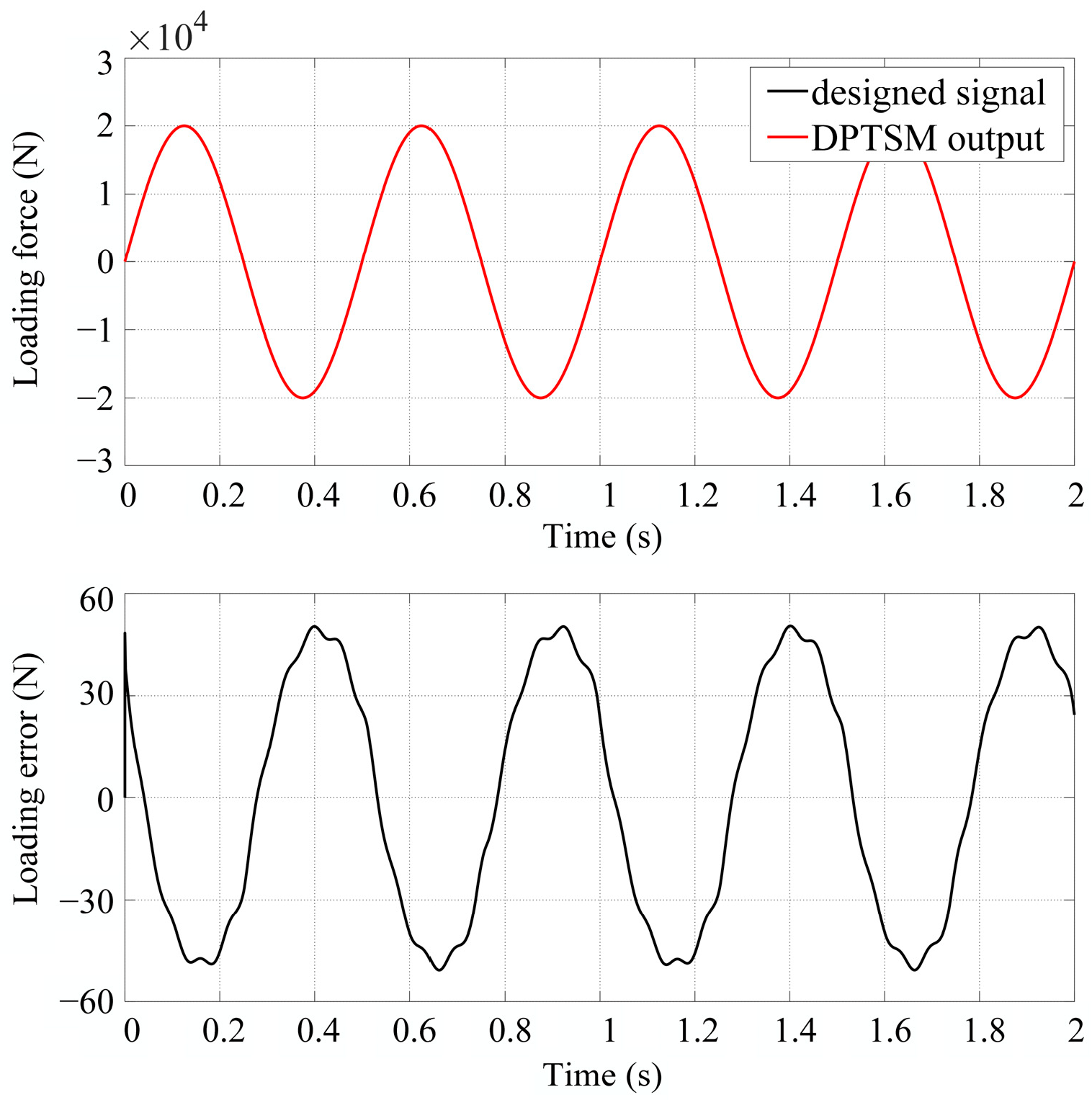
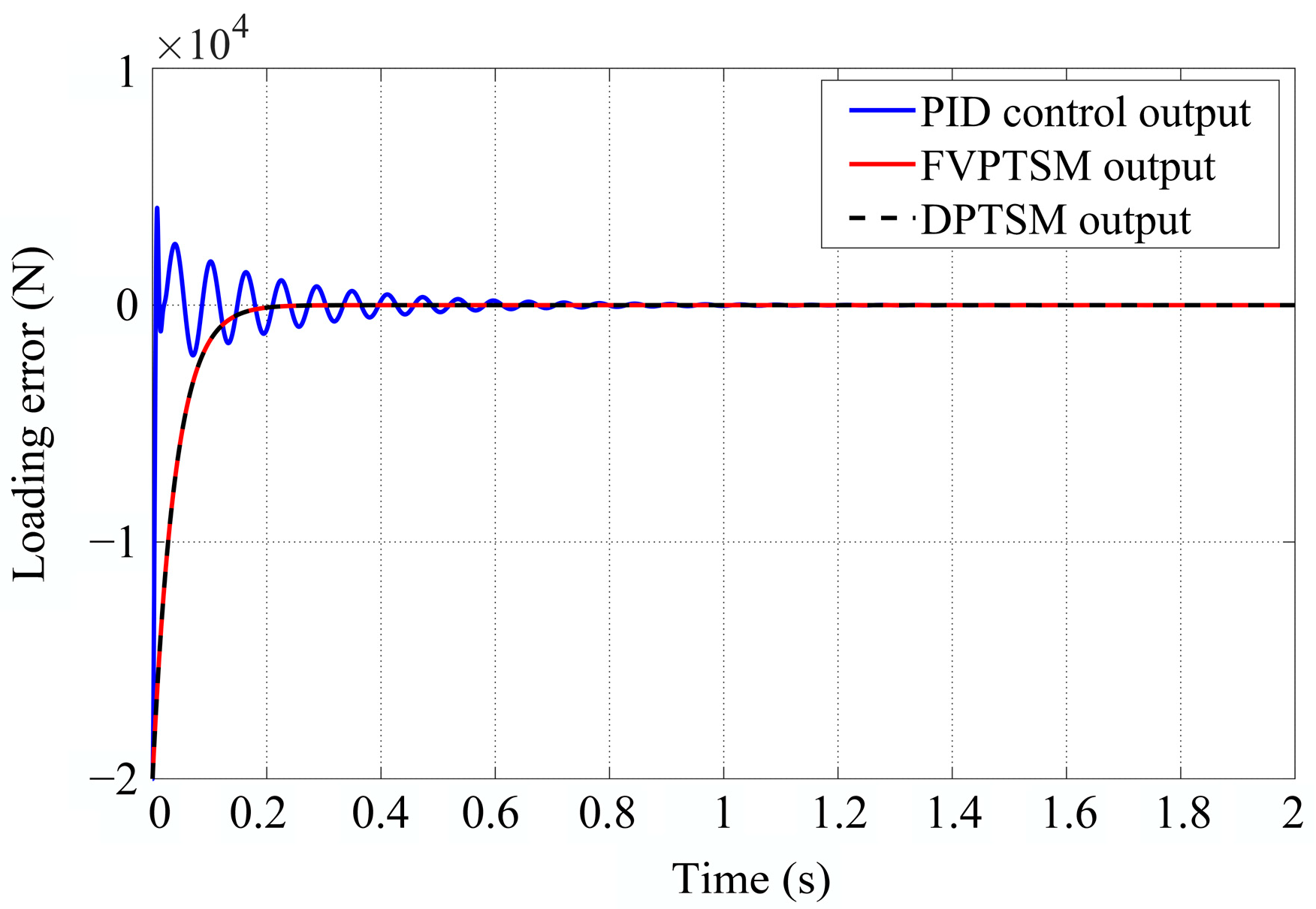
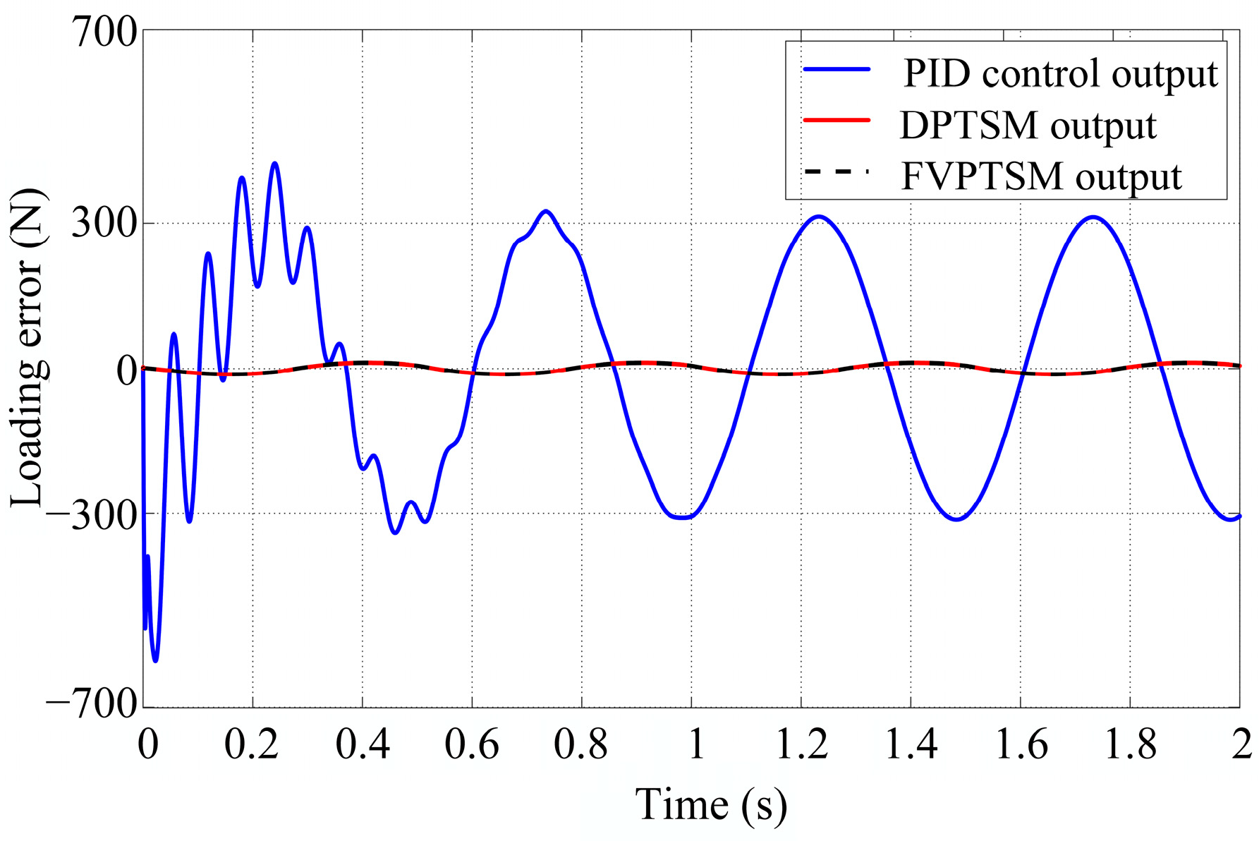
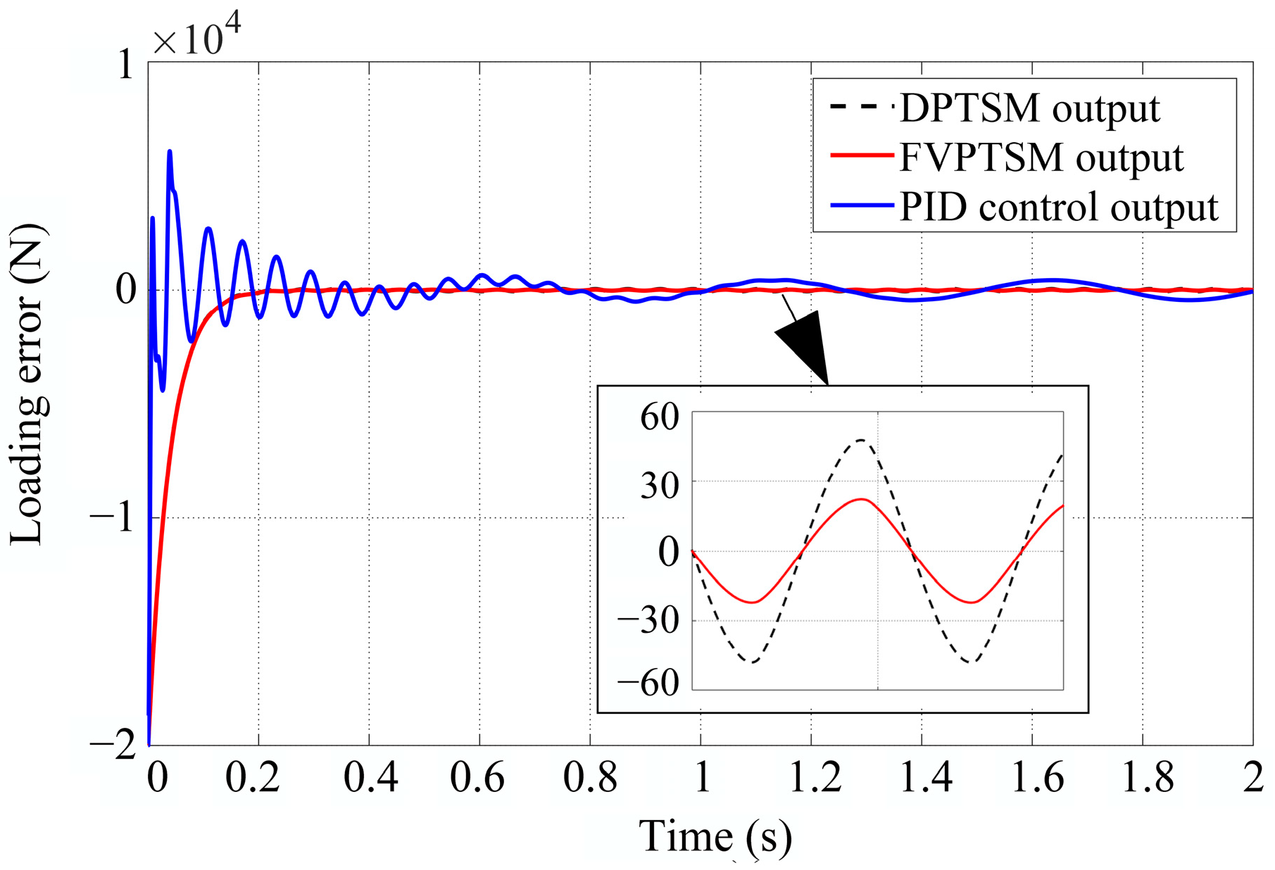
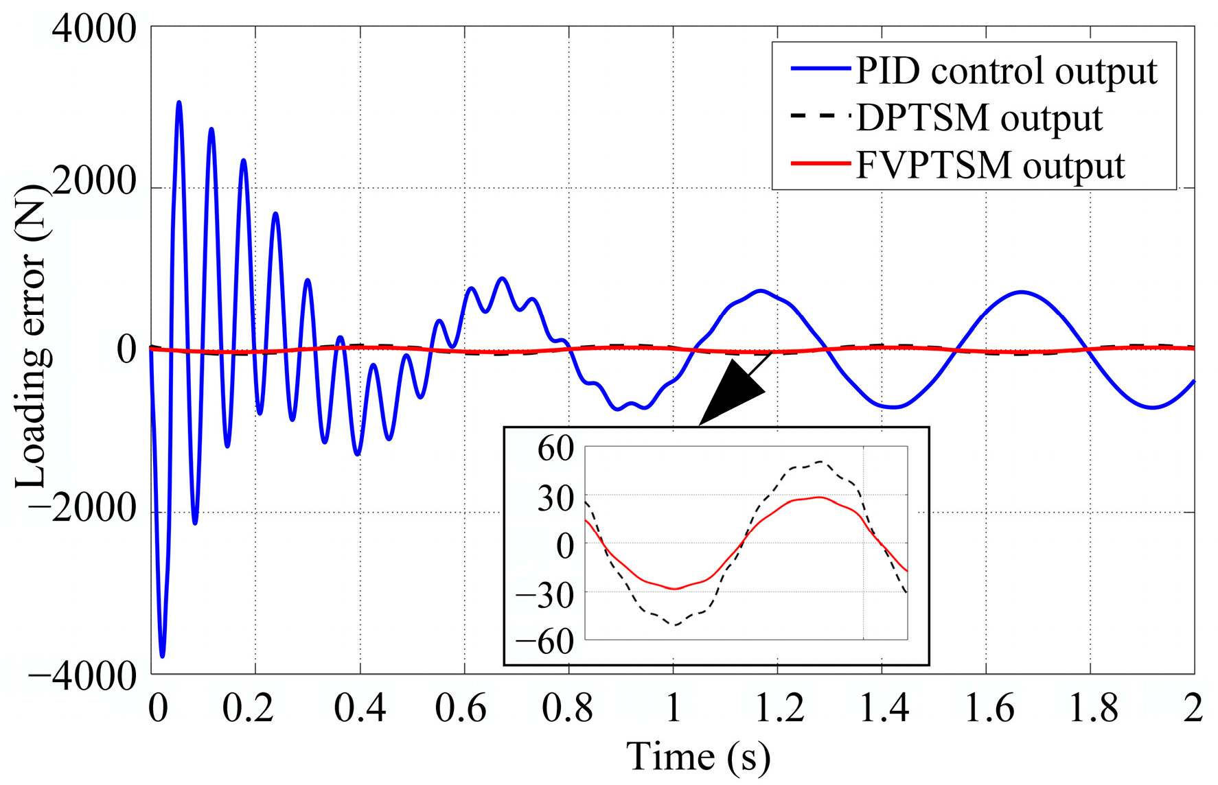
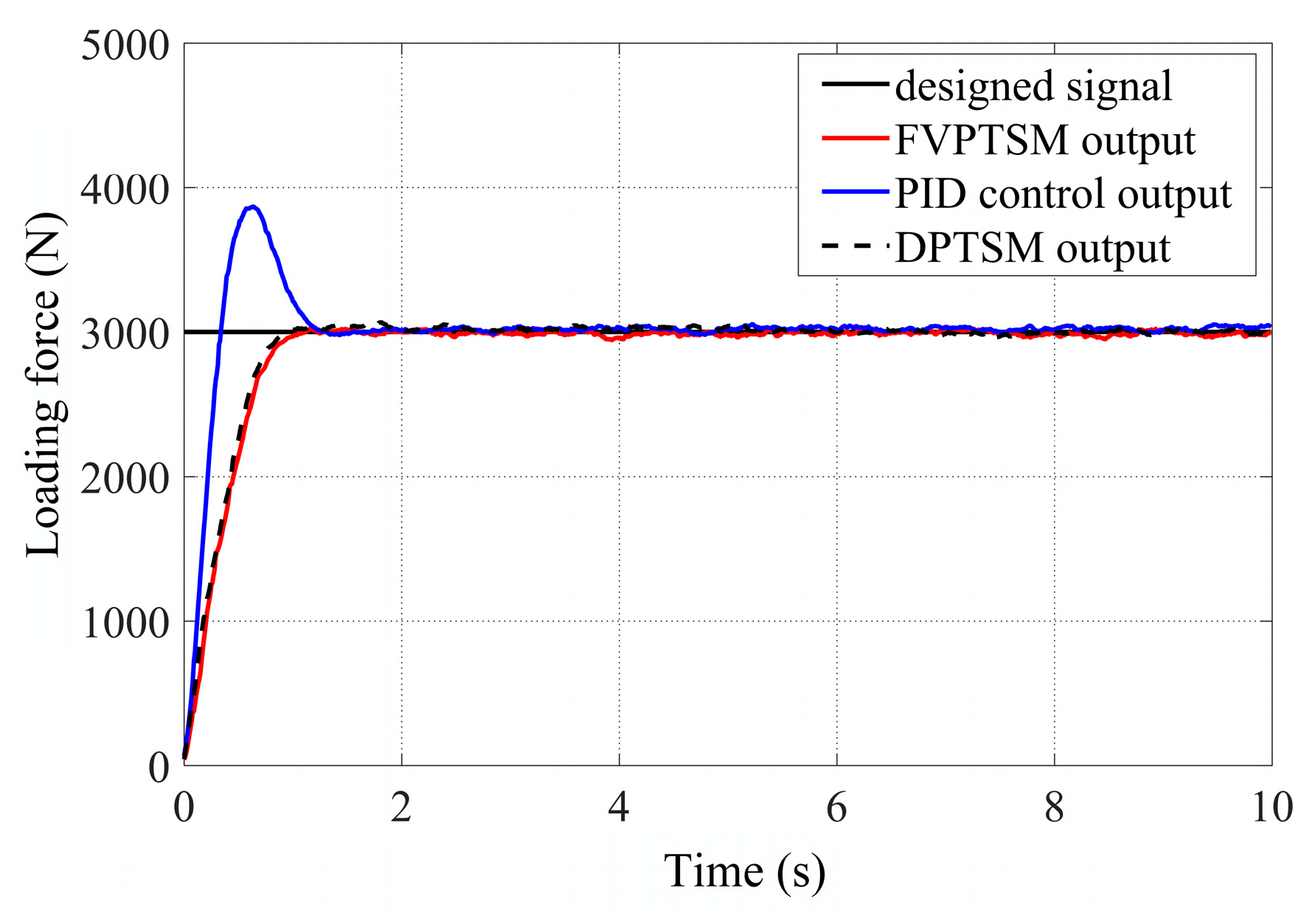
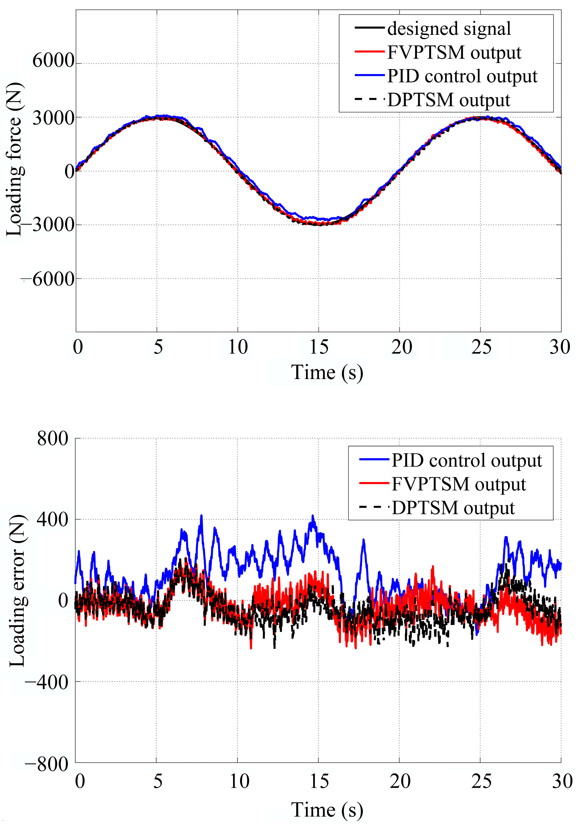
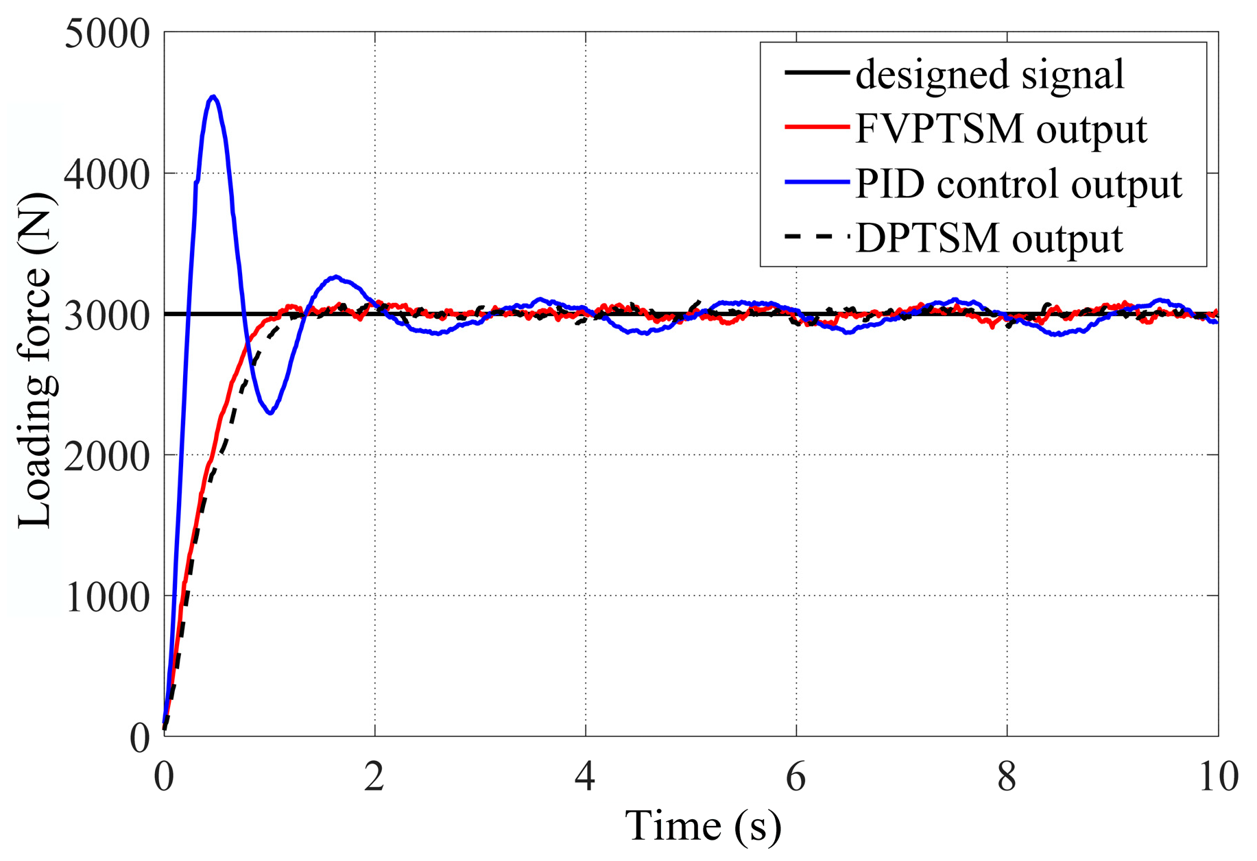
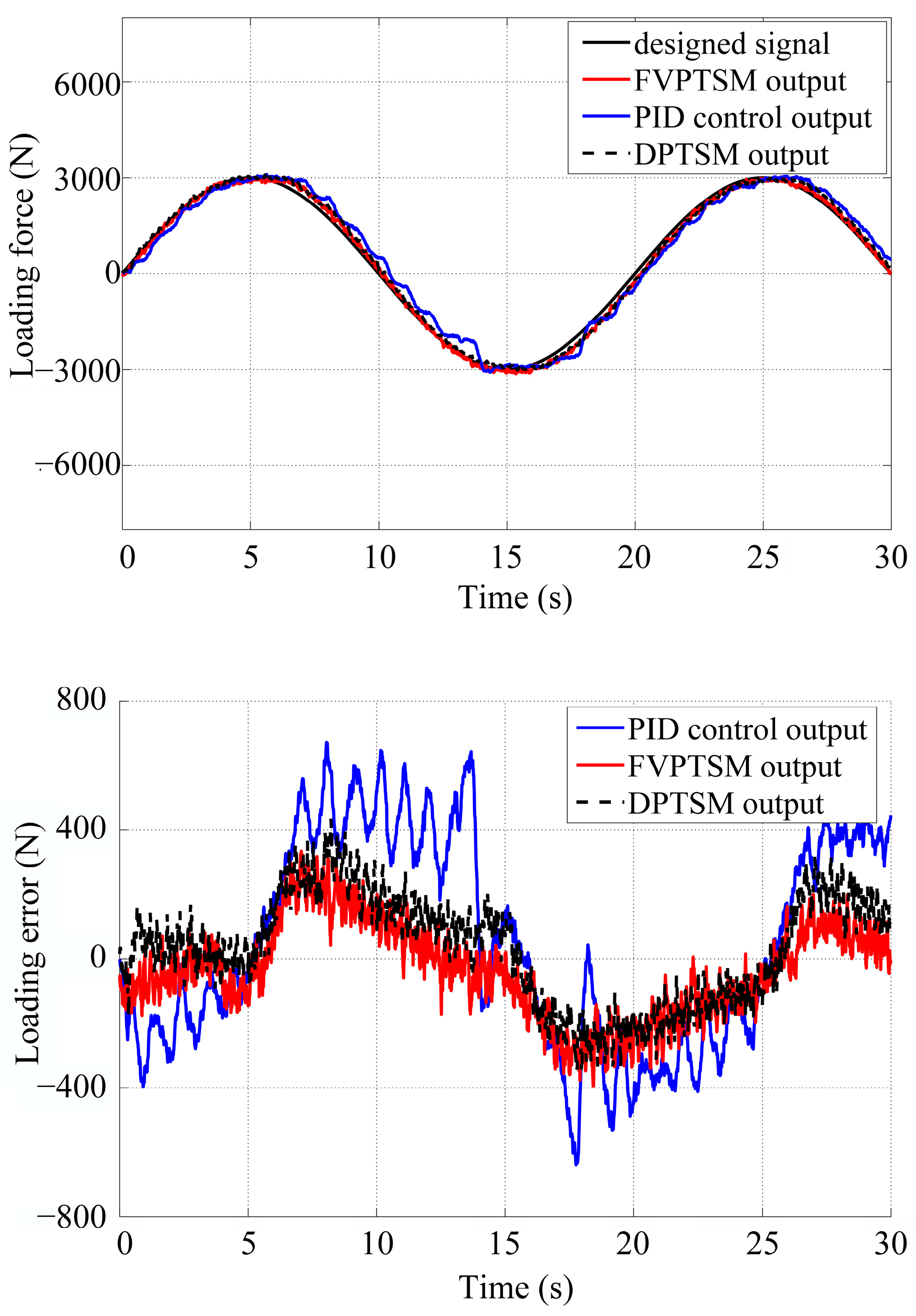
The controllers of the FVPTSM, the derived double-power terminal sliding mode control (DPTSM), and the PID are designed for conducting a comparison of the simulation and experimental verification, and the results demonstrate the effectiveness of the proposed strategy.

2. System Introduction and Mathematical Model

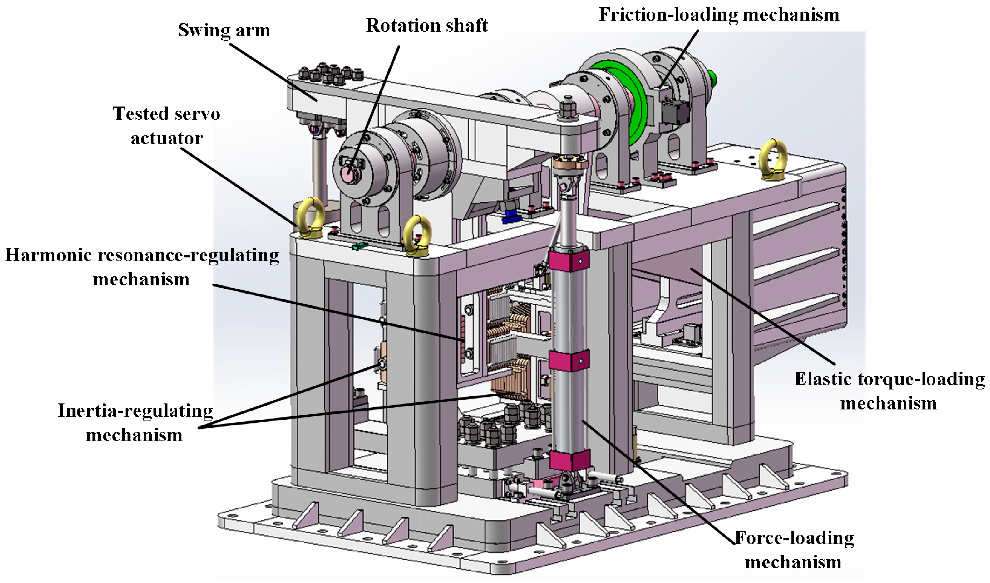
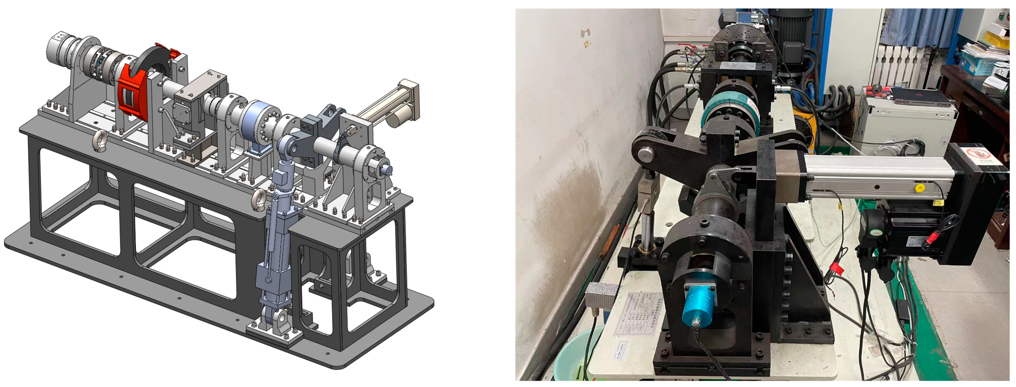
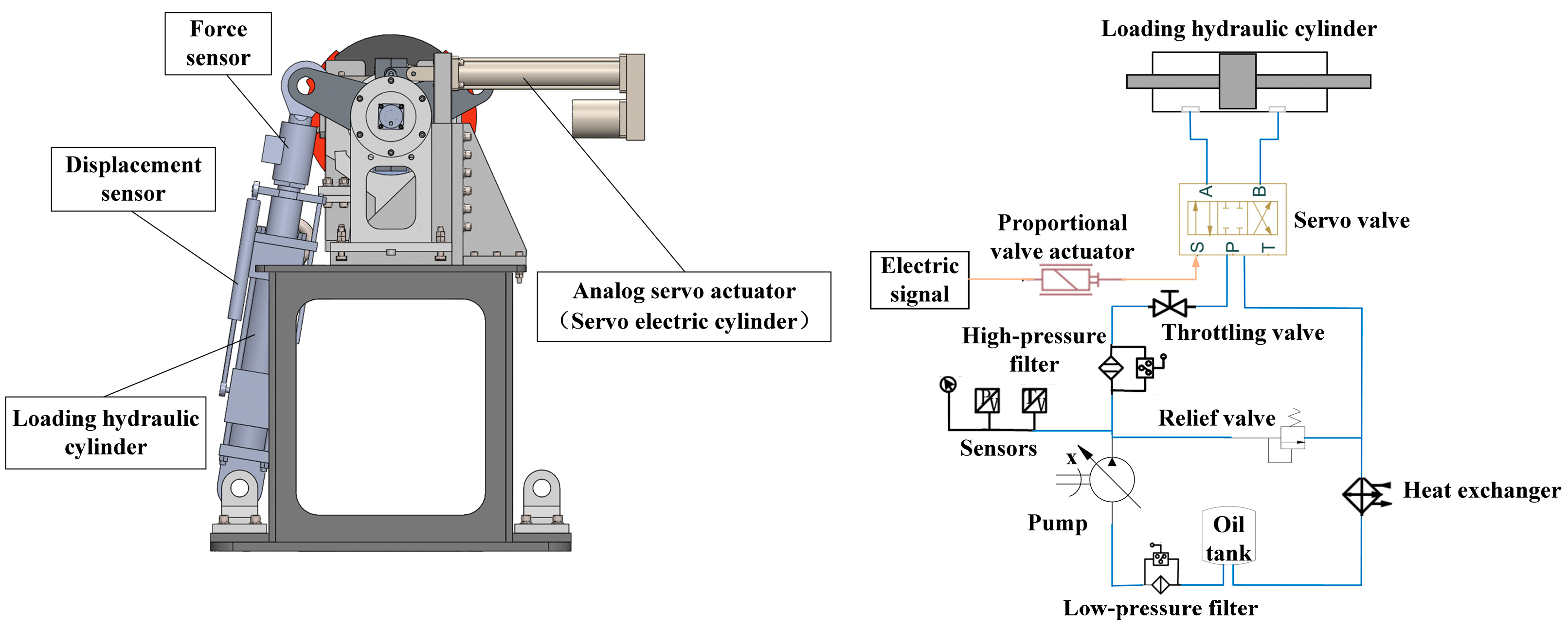
2.1. Mechanical Structure and Construction of the System

An aerospace electro-hydraulic load simulation system is used to simulate the ground dynamic and static performance test, research test, and servo control algorithm verification of the high-power servomechanism. Therefore, this system is required to provide loading test conditions of complex dynamic variables that are close to the real load object. The system also must provide force loading with high accuracy.

The simulator is composed of a tested servo actuator, force-loading mechanism, friction-loading mechanism, elastic torque-loading mechanism, inertia-regulating mechanism, and harmonic resonance-regulating mechanism, as shown in Figure 1. The designed simulator is a large-load, high-inertia servo system with a loading force range of ±20 kN and an inertia value of 2200 kg.m².

The friction-loading mechanism is installed on the rotating shaft that is used to simulate the damping characteristic. The elastic torque-loading mechanism and inertia-regulating mechanism fixed on the cantilever constitute the elastic constant and equivalent mass of rotation of the load simulation system. The harmonic resonance is adjusted through the design of the primary and secondary mass block. The tested servo actuator and the force-loading mechanism are installed at the end of the swing arm, respectively, which are both closed-loop systems comprising the servo valve and double-rod cylinder. Due to the force coupling through the swing arm, position interference is generated by the active motion of the actuator, while the force-loading unit loads the force to the servo actuator.

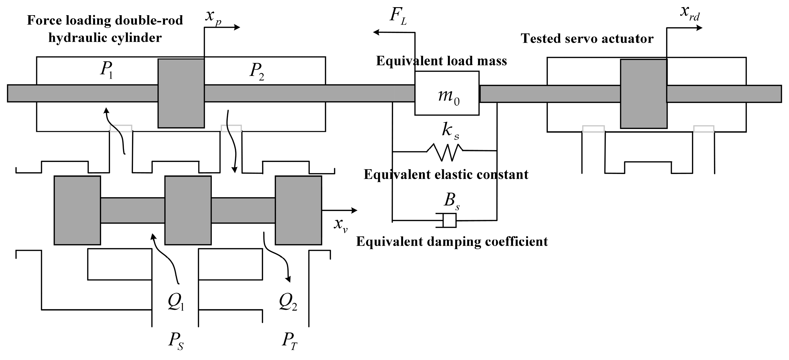
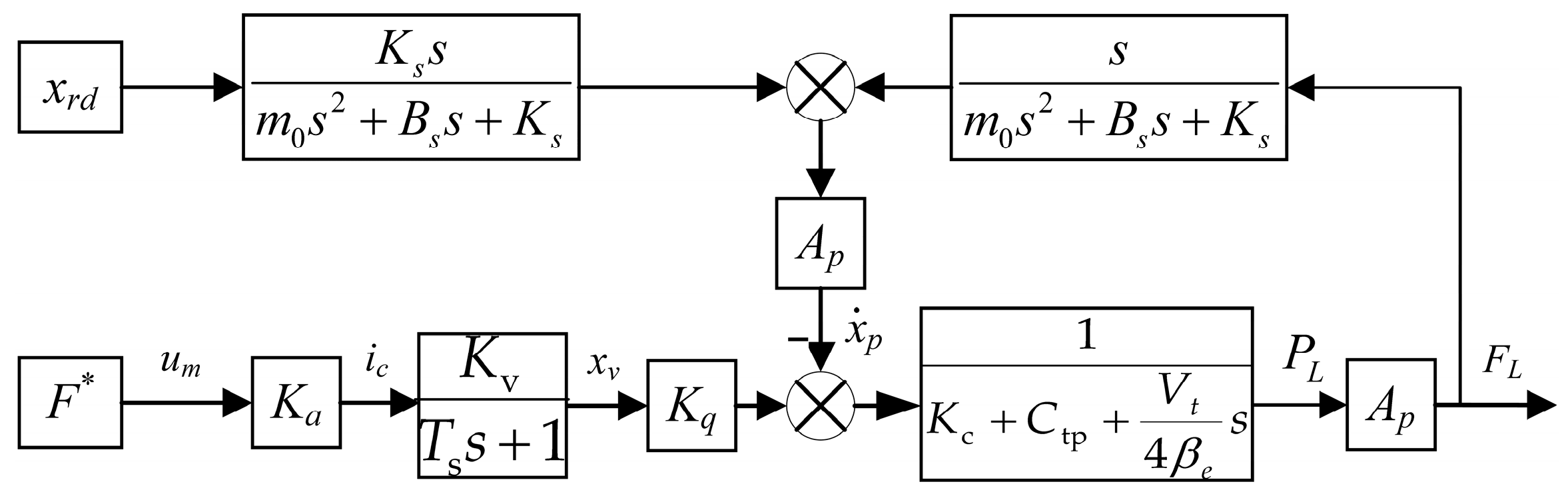
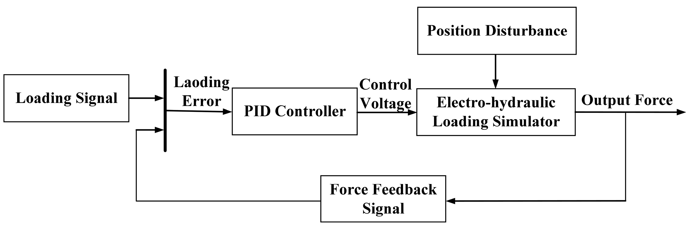
2.2. Mathematical Model of Force Loading System

The force-loading servomechanism loads the force to the tested servo actuator by way of the force coupling of the swing arm. The inertia-regulating mechanism, elastic torque-loading mechanism, and friction-loading mechanism are equivalent to the load mass, the elastic constant, and damping coefficient in the system, respectively, as shown in Figure 2. To ensure the precision of the loading force acting on the tested servo actuator in a short time, the servo valve controlling the double-rod symmetrical hydraulic cylinder is employed in the force-loading mechanism, in which voltage and force represent the input and output, respectively.

The idealized assumptions for the valve and hydraulic cylinder are outlined as follows:

(1)

The valve is a four-way spool valve with an ideal opening, where the four throttling windows are matched and symmetrical;

(2)

The flow at the throttling window is turbulent flow, and the influence of liquid compressibility in the valve can be neglected;

(3)

The valve has an ideal response capability, that is, the flow change corresponding to the change of spool displacement and valve pressure drop can occur instantaneously;

(4)

The hydraulic cylinder is the ideal double-rod symmetrical hydraulic cylinder;

(5)

The oil supply pressure $p_s$ is constant, and the oil return pressure $p_T$ is zero.

According to the small-hole throttle formula and flow continuity equation, the flow equation of the inlet and outlet chambers of the oil of the force load mechanism can be written as follows:

$$Q_1=C_d{A}_1\sqrt{\frac{2(p_s-p_1)}{\rho }}$$

(1)

$$Q_2=C_d{A}_2\sqrt{\frac{2p_2}{\rho }}$$

(2)

where $Q_1$ and $Q_2$ are the flow of the two chambers, $C_d$ is the discharge coefficient, $A_1$ and $A_2$ are the throttling window area of the servo valve spool, $p_s$ is the supply pressure, $\rho$ is the density of hydraulic oil, and $p_1$ and $p_2$ are the pressure of the two chambers.

Due to the symmetry and matching of the four throttling windows of the servo valve, the area can be expressed as:

$$A_1=A_2=w{x}_v$$

(3)

where $w$ is the servo valve spool area gradient and $x_v$ is the servo spool displacement.

The load flow $Q_L$ and the load pressure $p_L$ are defined as follows:

$$Q_L=\frac{1}{2}(Q_1+Q_2)$$

(4)

$$p_L=p_1-p_2$$

(5)

Considering that the compressibility of the two chambers has little effect on the valve coefficient of the throttle window, and the external leakage of the hydraulic cylinder can be neglected, the following equation is still applicable.

$$p_S=p_1+p_2$$

(6)

Combining Equations (1)–(3), (5) and (6), Equations (7) and (8) can be derived as shown below.

$$K_q=\frac{\partial Q_1}{\partial x_v}=\frac{\partial Q_2}{\partial x_v}{=C}_{d}w\sqrt{\frac{p_s-p_L}{\rho }}$$

(7)

$$2K_c=-\frac{\partial Q_1}{\partial p_1}=\frac{\partial Q_2}{\partial p_2}=C_{d}w{x}_v\sqrt{\frac{1}{\rho (p_s-p_L)}}$$

(8)

where $K_q$ is the flow gain and $K_c$ is the flow pressure coefficient.

Therefore, the linearized flow equation of the two throttling windows of the spool valve can be written as follows:

$${∆Q}_1=K_q∆x_v-2K_c∆P_1$$

(9)

$${∆Q}_2=K_q∆x_v+2K_c∆P_2$$

(10)

By the addition of Equations (9) and (10) combined with Equations (4) and (5), the increment of load flow can be derived as:

$${∆Q}_L=\frac{1}{2}(∆Q_1+∆Q_2){=K}_q∆x_v-K_c∆P_L$$

(11)

To simplify the derivation of the flow continuity equation, the following assumptions are made:

(1)

All connecting pipes are short and thick, and the friction loss, liquid quality, and dynamic properties of the oil circuit can be neglected;

(2)

The internal pressure of each chamber of the hydraulic cylinder is equal everywhere, and the oil temperature and volume elastic modulus can be considered to be constant;

(3)

The internal and external leakage of the hydraulic cylinder is in the form of laminar flow.

Based on the abovementioned assumptions, the flow continuity equation of the inlet and outlet chambers of the oil in the hydraulic cylinder can be written as:

$$Q_1=A_p\frac{d{x}_p}{dt}+C_{ip}(P_1-P_2)+C_{ep}{P}_1+\frac{V_1}{{\beta }_e}\frac{d{p}_1}{dt}$$

(12)

$$Q_2=A_p\frac{d{x}_p}{dt}+C_{ip}(P_1-P_2)-C_{ep}{P}_2-\frac{V_2}{{\beta }_e}\frac{d{p}_2}{dt}$$

(13)

where $A_p$ is the effective area of the hydraulic cylinder piston, $x_p$ is the piston displacement of the loading hydraulic cylinder, $C_{ip}$ and $C_{ep}$ are the internal and external leakage coefficients of the hydraulic cylinder, $V_1$ and $V_2$ are the volume of the oil inlet and outlet chambers, respectively, and ${\beta }_e$ is the equivalent volume elastic modulus of hydraulic oil.

Assuming that the hydraulic cylinder is operated at the middle position, the initial volumes of the two chambers are expressed in the equation $V_{01}=V_{02}=\frac{Vt}{2}$, where $V_t$ is the total volume of the two chambers. Therefore, $V_1$ and $V_2$ can be expressed as:

$$V_1=V_{01}+x_p{A}_p=\frac{Vt}{2}+x_p{A}_p$$

(14)

$$V_2=V_{02}-x_p{A}_p=\frac{Vt}{2}-x_p{A}_p$$

(15)

Combined with Equations (4) and (5), the load flow equation can be obtained as:

$$Q_L=\frac{1}{2}(Q_1+Q_2)=A_p\frac{d{x}_p}{dt}+(C_{ip}+\frac{C_{ep}}{2})P_L+\frac{V_t}{{4\beta }_e}\frac{d{p}_L}{dt}+\frac{x_p{A}_p}{{2\beta }_e}(\frac{d{p}_1}{dt}+\frac{d{p}_2}{dt})$$

(16)

The equation $\frac{d{p}_1}{dt}=-\frac{d{p}_2}{dt}$ can be obtained through Equations (5) and (6). Therefore, the flow continuity equation can be simplified as:

$$Q_L=\frac{1}{2}(Q_1+Q_2)=A_p\frac{d{x}_p}{dt}+C_{tp}{P}_L+\frac{V_t}{{4\beta }_e}\frac{d{p}_L}{dt}$$

(17)

where $C_{tp}=C_{ip}+\frac{C_{ep}}{2}$ is the total leakage coefficient of the hydraulic cylinder, $A_p\frac{d{x}_p}{dt}$ is the flow required to drive the piston movement of the hydraulic cylinder, $C_{tp}{P}_L$ is the total leakage flow, and $\frac{V_t}{{4\beta }_e}\frac{d{p}_L}{dt}$ is the compression flow.

Due to the force coupling of the force-loading servomechanism and tested servo actuator, as shown in Figure 2, Equation (18) can be established according to Newton second flow.

$$A_p{P}_L=m_0\frac{d^2{x}_p}{d{t}^2}+B_s\frac{d{x}_p}{dt}+K_s\left(x_p-x_{rd}\right)$$

(18)

where $m_0$ is the equivalent mass of the system inertia, $B_s$ is the equivalent viscous damp coefficient, including the friction between the piston rod and the servo hydraulic cylinder of the force-loading and friction-loading mechanisms, $K_s$ is the equivalent elastic constant of the elastic torque-loading mechanism, and $x_{rd}$ is the displacement of the position disturbance of the tested servo actuator.

Considering that the frequency width of the aerospace electro-hydraulic load simulation system in this paper is far lower than that of the electro-hydraulic servo valve, the servo valve can be regarded as the first-order inertia element. Hence, the relationship of the control voltage and the servo spool displacement can be described as:

$$\dot{x_v}=-w_n{x}_v+K_v{K}_a{w}_n{u}_m$$

(19)

where $K_v$ is the gain coefficient of the servo valve, $K_a$ is the gain coefficient of the input voltage and the output current of the linear force motor of the servo force, $w_n$ is the natural frequency of the servo valve, $u_m$ is the control input voltage, and $x_v$ is the servo spool displacement of the servo valve.

Combining Equations (11) and (17)–(19), the open-loop transfer function can be derived in the form of Equation (20), and the block diagram of the open-loop transfer function is depicted in Figure 3.

$$A_p{P}_L=\frac{\frac{A_p{K}_q}{K_{ce}}\left(\frac{m_0}{K_s}{S}^2+\frac{B_s}{K_s}S+1\right)x_v-\frac{{A_p}^{2}S}{K_{ce}}{x}_{rd}}{\frac{{V_{t}m}_0}{{4\beta }_e{K}_s{K}_{ce}}{S}^3+\left(\frac{B_s{V}_t}{{4\beta }_e{K}_s{K}_{ce}}+\frac{m_0}{K_s}\right)S^2+\left(\frac{V_t}{{4\beta }_e{K}_{ce}}+\frac{{A_p}^2}{K_s{K}_{ce}}+\frac{B_s}{K_s}\right)s+1}$$

(20)

where $K_{ce}$ is the total flow pressure coefficient of the system, and $K_{ce}=K_c+C_{tp}$.

As depicted in Figure 3, the surplus force is induced by the differential effect of $x_{rd}$, where $x_{rd}$ is the displacement of the position disturbance of the tested servo actuator. According to Equation (20), the differential term of $x_{rd}$ causes the surplus force. Due to the high-frequency sensitivity characteristic of the differential term, a high-frequency position disturbance usually results in a large surplus force. Meanwhile, due to the leading characteristic of the surplus force caused by the active disturbance of the tested servo actuator, the output force $F_L$ of the electro-hydraulic loading mechanism always lags behind the surplus force. Given the effect of the phase lag of the high inertia and the higher inertia induced by the larger mass, the phase lag is positively correlated with the increase in the equivalent mass $m_0$. Therefore, the designed control strategy needs to overcome the position interference and the large phase lag problem of the system to ensure the accuracy of the force tracking, under the premise of not only ensuring the robustness of the system but also realizing the fast convergence of the system.

3. Proposal and Implementation of the Terminal Sliding Mode Control Strategy Based on the Modified Fast Double-Power Reaching Law

3.1. The State–Space Model of Force-Loading System

Considering the piston displacement of the loading hydraulic cylinder $x_p$, the piston velocity $\dot{x_p}$, the load pressure $p_L$, and the servo spool displacement $x_v$ as the state variables, the state vector of the system can be defined as

$$x=\left[x_1{x}_2{x}_3{x}_4\right]=\left[x_p\dot{x_p}{p}_L{x}_v\right]$$

(21)

Based on Equations (11), (17)–(19) and (21), and defining $u_m$ as the system input and $p_L$ as the system output, where $p_L=\frac{F_L}{A_p}$, and $F_L$ is the load force of the loading hydraulic mechanism, the entire system of the load simulator can be deduced in the state–space form as:

$$x=\left\{\begin{array}{l}\dot{x_1}=x_2\\ \dot{x_2}=\frac{1}{m_0}\left(-K_s{x_1-B_{s}x}_2+A_p{x}_3+K_s{x}_{rd}\right)\\ \dot{x_3}=\frac{{4\beta }_e}{V_t}\left(-A_p{x}_2-K_{ce}{x}_3+K_q{x}_4\right)\\ \dot{x_4}=-w_n{x}_4+K_v{K}_a{w}_n{u}_m\end{array}\right.$$

(22)

To simplify the discussion and derivation process, ${\lambda }_i,\left(i=1,2,\dots ,7\right)$ and $F_{rd}$ are defined as:

$$\left\{\begin{array}{l}{\lambda }_1=\frac{B_s}{m_0}\\ {\lambda }_2=\frac{A_p}{m_0}\\ {\lambda }_3=\frac{{4\beta }_e{K}_q}{V_t}\\ {\lambda }_4=\frac{{4\beta }_e{A}_p}{V_t}\\ {\lambda }_5=\frac{{4\beta }_e{K}_{ce}}{V_t}\\ {\lambda }_6=w_n\\ {\lambda }_7=K_v{K}_a{w}_n\\ F_{rd}=\frac{K_s\left(x_{rd}-x_p\right)}{m_0}\end{array}\right.$$

(23)

Based on the abovementioned definition, the state–space model of the system can be transformed to:

$$x=\left\{\begin{array}{l}\dot{x_1}=x_2\\ \dot{x_2}=-{\lambda }_1{x}_2+{\lambda }_2{x}_3+F_{rd}\\ \dot{x_3}={\lambda }_3{x}_4-{\lambda }_4{x}_2-{\lambda }_5{x}_3\\ \dot{x_4}=-{\lambda }_6{x}_4+{\lambda }_7{u}_m\end{array}\right.$$

(24)

With load pressure $p_L$ as the system output, the system error $e$ can be expressed as:

$$e=x_3-{x_3}^{*}$$

(25)

where ${x_3}^{*}$ is the desired load pressure of the system output.

3.2. FVPTSM Controller Design

The sliding mode control (SMC) is a type of variable structure control, where the system’s structure is not fixed. The structure of the system can be accordingly modified during the dynamic process based on the current state of the system, such as the deviation and its various derivatives. This compels the system to follow the state trajectory of predetermined sliding mode dynamics. Therefore, the SMC exhibits the advantages of strong robustness, a fast response, the non-necessity of online identification, and simple physical implementation. Based on the abovementioned features, the introduction of the SMC into the controller design of the electro-hydraulic load simulator is feasible and suitable. Due to the contradiction between the chattering issue and fast convergence of the SMC, the combination of the modified fast variable-power reaching law (MFVP) and a nonsingular fast terminal (NFT) SMC, which is abbreviated as FVPTSM, is proposed for the implementation of the controller.

To suppress the chattering issue and realize the convergence to the sliding surface in finite time, an SMC based on the MFVP is adopted in the form of Equation (26).

$$\dot{s}=-k_1{\left|s\right|}^{\theta }sgn\left(s\right)-k_2{\left|s\right|}^{{\alpha }_2}sgn\left(s\right)-k_{3}s$$

(26)

where $k_1$, $k_2$, $k_3$, ${\alpha }_1$, and ${\alpha }_2$ are the tuning parameters of the reaching law with the definitions of $\theta ={\alpha }_1$ when $\left|s\right|\ge 1$, and $\theta =1$ when $\left|s\right|<1$, while satisfying the conditions of $k_1>0$, $k_2>0$, $k_3>0$, ${\alpha }_1>1$, and ${0<\alpha }_2<1$.

When $\left|s\right|\ge 1$, the reaching law can be transformed to:

$$\dot{s}=-k_1{\left|s\right|}^{{\alpha }_1}sgn\left(s\right)-k_2{\left|s\right|}^{{\alpha }_2}sgn\left(s\right)-k_{3}s$$

(27)

From Equation (27), it can be seen that the reaching law equals the combination of the double-power reaching law and the exponential reaching law. Due to the addition of the exponential term in comparison to the double-power reaching law, the system obtains a higher reaching speed when the system state is far from the sliding mode surface, shortening the system response time and improving the response velocity.

The form of the reaching law can be described in the form of Equation (28) in the circumstance of $\left|s\right|<1$.

$$\dot{s}=-k_2{\left|s\right|}^{{\alpha }_2}sgn\left(s\right)-(k_1+k_3)s$$

(28)

It can be observed that the current reaching law is equivalent to a combination of the power and exponential laws from Equation (28). Compared to the single-power reaching law, the incorporation of the exponential term allows for the selection of larger values of $k_1$ and $k_3$ to ensure faster convergence rates, and a smaller value of ${\alpha }_2$ to smoothly enter into the sliding mode and effectively reduce chattering. Therefore, it exhibits superior dynamic characteristics when dealing with external disturbances.

To address the singularity caused by a zero system state, due to the inclusion of a negative power term of the system state in the controller design of the traditional fast terminal sliding mode and the asymptotic convergence of the linear sliding mode surface, the nonsingular fast terminal sliding surface is selected as per the following expression:

$$s=x+\frac{1}{\beta }{\dot{x}}^{\frac{p}{q}}$$

(29)

where $x$ is the state variable, $\beta$, $p$, and $q$ are the tuning parameters of the sliding surface, and $\beta >0$. $1<\frac{p}{q}<2$, where $p$ and $q$ are the positive odd numbers.

The motion of the SMC can be divided into approach and sliding motions. Therefore, this paper creatively introduces a controller that simultaneously satisfies Equations (26) and (29) in order to achieve finite-time convergence, as well as guaranteeing an excellent dynamic quality and static precision in each motion process.

The Lyapunov function is defined as:

$$V=\frac{1}{2}{s}^2$$

(30)

Considering the differentiation of Equation (30) and combining it with Equation (29) and the equation $x=e$, where $x$ is the state variable of the NFT and $e$ is the system error, jointing the state–space model and the error definition of the system yields:

$$\begin{array}{l}\dot{V}=s\dot{s}\hfill \\ =s(\dot{x}+\frac{p}{\beta q}{\dot{x}}^{\left(\frac{p}{q}-1\right)}\ddot{x})\\ =s(\dot{e}+\frac{p}{\beta q}{\dot{e}}^{\left(\frac{p}{q}-1\right)}\ddot{e})\\ =s(\dot{e}+\frac{p}{\beta q}{\dot{e}}^{\left(\frac{p}{q}-1\right)}(\ddot{x_3}-\ddot{{x_3}^{*}}\left)\right)\\ =s(\dot{e}+\frac{p}{\beta q}{\dot{e}}^{\left(\frac{p}{q}-1\right)}({\lambda }_3\dot{x_4}-{\lambda }_4\dot{x_2}-{\lambda }_5\dot{x_3}-\ddot{{x_3}^{*}}\left)\right)\\ =s(\dot{e}+\frac{p}{\beta q}{\dot{e}}^{\left(\frac{p}{q}-1\right)}({\lambda }_3(-{\lambda }_6{x}_4+{\lambda }_7{u}_m)-{\lambda }_4\dot{x_2}-{\lambda }_5\dot{x_3}-\ddot{{x_3}^{*}}\left)\right)\end{array}$$

(31)

To satisfy the convergence process of either case and simplify the solution, the total controller $u_m$ can be decomposed into two components, $u_1$ and $u_2$, as follows.

$$u_m=u_1+u_2$$

(32)

where the role of the controller $u_1$ is that the system state converges to the equilibrium point along the nonsingular fast terminal sliding surface, thus necessitating the establishment of the equation $\dot{e}+\frac{p}{\beta q}{\dot{e}}^{\left(\frac{p}{q}-1\right)}\left({\lambda }_3\right(-{\lambda }_6{x}_4+{\lambda }_7{u}_m)-{\lambda }_4\dot{x_2}-{\lambda }_5\dot{x_3}-\ddot{{x_3}^{*}})=0$. The expression $u_1$ is obtained in the following form:

$$u_1=\frac{1}{{\lambda }_3{\lambda }_7}(-\frac{\beta q}{p}{\dot{e}}^{\left(2-\frac{p}{q}\right)}+{\lambda }_3{\lambda }_6{x}_4+{\lambda }_4\dot{x_2}+{\lambda }_5\dot{x_3}+\ddot{{x_3}^{*}})$$

(33)

The controller $u_2$ is used to ensure the system’s dynamic and static quality of approaching motion according to Equation (26), which is deduced by the MFVP. Therefore, $u_2$ can be obtained in the form of:

$$u_2=\frac{1}{{\lambda }_3{\lambda }_7}(-k_1{\left|s\right|}^{\theta }sgn(s)-k_2{\left|s\right|}^{{\alpha }_2}sgn(s)-k_{3}s)$$

(34)

Based on Equations (33) and (34), the combination controller $u_m$ of the MFVP and NFT can be expressed as:

$$u_m=\frac{1}{{\lambda }_3{\lambda }_7}(-\frac{\beta q}{p}{\dot{e}}^{\left(2-\frac{p}{q}\right)}+{\lambda }_3{\lambda }_6{x}_4+{\lambda }_4\dot{x_2}+{\lambda }_5\dot{x_3}+\ddot{{x_3}^{*}}-k_1{\left|s\right|}^{\theta }sgn(s)-k_2{\left|s\right|}^{{\alpha }_2}sgn(s)-k_{3}s)$$

(35)

3.3. Finite-Time Proof and Stability Analysis

Theorem 1. 

For the aerospace electro-hydraulic load simulator (22), including the bounded displacement disturbance and the strong phase lag, under the controller as shown in Equation (35), the force tracking error of the simulator can converge to a small neighbor range of the system’s equilibrium point in finite time, and the system is asymptotically stable.

Proof of Theorem 1. 

Assuming that the system state varies from the arbitrary initial state $x\left(0\right)\ne 0$ to the equilibrium point $x=0$ along the sliding surface as shown in Equation (29) with $x=e$, the following expression can be obtained:

$$e+\frac{1}{\beta }{\dot{e}}^{\frac{p}{q}}=0$$

(36)

Computing the definite integral of the above equation yields:

$${\int }_0^{t}dt={\int }_{e\left(0\right)}^0-{\beta }^{-\frac{q}{p}}{e}^{-\frac{q}{p}}de$$

(37)

Subsequently, the convergence time can be obtained as:

$$t_s={\beta }^{-\frac{q}{p}}\frac{p}{p-q}{\left|e\right(0\left)\right|}^{1-\frac{q}{p}}$$

(38)

It can be concluded that the nonsingular fast terminal SMC not only improves the convergence velocity in the vicinity of the equilibrium state, but also enhances the velocity at locations that are far away from the equilibrium point. This feature enables the system to reach equilibrium in finite time.

Substituting Equation (35) into Equation (31), the differentiation of the Lyapunov function yields:

$$\dot{V}=\frac{p}{\beta q}{\dot{e}}^{\left(\frac{p}{q}-1\right)}(-k_1{\left|s\right|}^{\theta }sgn(s)-k_2{\left|s\right|}^{{\alpha }_2}sgn(s)-k_{3}s)$$

(39)

Since $1<\frac{p}{q}<2$, $0<\frac{p}{q}-1<1$, and combining it with $\beta >0$ and the positive odd numbers $p$ and $q$, the inequality $\frac{p}{\beta q}{\dot{e}}^{\left(\frac{p}{q}-1\right)}>0$ can be obtained when $\dot{e}\ne 0$. In order to simplify the subsequent derivations, we define ${k_1}^{/}=\frac{p}{\beta q}{\dot{e}}^{\left(\frac{p}{q}-1\right)}{k}_1$, ${k_2}^{/}=\frac{p}{\beta q}{\dot{e}}^{\left(\frac{p}{q}-1\right)}{k}_2$, and ${k_3}^{/}=\frac{p}{\beta q}{\dot{e}}^{\left(\frac{p}{q}-1\right)}{k}_3$. Equation (39) can be transformed to

$$\dot{V}=-{k_1}^{/}{\left|s\right|}^{\theta }sgn\left(s\right)-{k_2}^{/}{\left|s\right|}^{{\alpha }_2}sgn\left(s\right)-{k_3}^{/}s$$

(40)

where ${k_1}^{/}>0$, ${k_2}^{/}>0$, and ${k_3}^{/}>0$ when $\dot{e}\ne 0$.

According to Equations (30) and (40), $V\ge 0$, $\dot{V}\le 0$ and $V=0$, $\dot{V}=0$ if and only if $s=0$, satisfying LaSalle’s invariance principle. Therefore, it is observed that the system is asymptotically stable during the process of approaching the sliding surface.

The approach motion of the system can be decomposed into three stages, namely $s=s_0$ to $s=1$, $s=1$ to $s={\alpha }_2$, and $s={\alpha }_2$ to $s=0$.

During the first stage, the reaching law can be expressed as:

$$\dot{s}=-k_1{\left|s\right|}^{{\alpha }_1}sgn\left(s\right)-k_2{\left|s\right|}^{{\alpha }_2}sgn\left(s\right)-k_{3}s$$

(41)

where $k_1={k_1}^{/}$, $k_2={k_2}^{/}$, and $k_3={k_3}^{/}$.

The approach process can be divided into two components in the form of:

$$\left\{\begin{array}{c}\dot{s}+k_1{\left|s\right|}^{{\alpha }_1}sgn\left(s\right)=-k_{3}s\\ \dot{s}+k_2{\left|s\right|}^{{\alpha }_2}sgn\left(s\right)=-k_{3}s\end{array}\right.$$

(42)

where $\dot{s}+k_1{\left|s\right|}^{{\alpha }_1}sgn\left(s\right)=-k_{3}s$ and $\dot{s}+k_2{\left|s\right|}^{{\alpha }_2}sgn\left(s\right)=-k_{3}s$ represent the influence of $k_1{\left|s\right|}^{{\alpha }_1}sgn\left(s\right)$ and $k_2{\left|s\right|}^{{\alpha }_2}sgn\left(s\right)$, respectively. Therefore, the approach time required for the entire system must be shorter than that of either of the aforementioned components, indicating that the approach time is less than the solution derived from either of the abovementioned two equations. Adopting $\dot{s}+k_1{\left|s\right|}^{{\alpha }_1}sgn\left(s\right)=-k_{3}s$ to compute the approach time results in the following equation.

$$\dot{s}+k_{3}s=-k_1{\left|s\right|}^{{\alpha }_1}sgn\left(s\right)$$

(43)

For further derivation, substituting the definition ${x=\left|s\right|}^{1-{\alpha }_1}$ and ${\dot{x}=(1-{\alpha }_1)\left|s\right|}^{-{\alpha }_1}$ into Equation (43) yields:

$$\dot{x}+k_3(1-{\alpha }_1)sgn\left(s\right)x=-k_1(1-{\alpha }_1)sgn\left(s\right)$$

(44)

According to the derivation formula of the first-order differential equation, $x$ can be obtained as:

$$x=C{e}^{-k_3(1-{\alpha }_1)sgn\left(s\right)t_1}-\frac{k_1}{k_3}$$

(45)

where $C$ is the constant awaiting resolution.

Due to the condition of $x={\left|s\right|}^{1-{\alpha }_1}$, $x$ can be rewritten as:

$${\left|s\right|}^{1-{\alpha }_1}=C{e}^{-k_3(1-{\alpha }_1)sgn\left(s\right)t_1}-\frac{k_1}{k_3}$$

(46)

When $t_1=0$, the value of $C$ can be solved as $C={\left|s_0\right|}^{1-{\alpha }_1}+\frac{k_1}{k_3}$. Substituting C into the equation yields:

$${\left|s\right|}^{1-{\alpha }_1}=({\left|s_0\right|}^{1-{\alpha }_1}+\frac{k_1}{k_3})e^{-k_3(1-{\alpha }_1)sgn\left(s\right)t_1}-\frac{k_1}{k_3}$$

(47)

On resolving the abovementioned equation, the approach time $t_1$ is given by the following expression.

$$t_1=\frac{1}{-k_3(1-{\alpha }_1)sgn\left(s\right)}\ln \frac{{\left|s\right|}^{1-{\alpha }_1}+\frac{k_1}{k_3}}{{\left|s_0\right|}^{1-{\alpha }_1}+\frac{k_1}{k_3}}$$

(48)

Because $s$ ranges from $s_0$ to 1, the value of $s$ is 1. The ultimate result of $t_1$ can be obtained as:

$$t_1=\frac{1}{k_3({\alpha }_1-1)}\ln \frac{1+\frac{k_1}{k_3}}{{\left|s_0\right|}^{1-{\alpha }_1}+\frac{k_1}{k_3}}$$

(49)

In the stage of $s$ varying from $s=1$ to $s={\alpha }_2$, the reaching law can be expressed as:

$$\dot{s}=-k_{1}s-k_2{\left|s\right|}^{{\alpha }_2}sgn\left(s\right)-k_{3}s$$

(50)

Similar to the first stage, the approach time required by this stage exceeds either of the influences of $k_{1}s+k_2{\left|s\right|}^{{\alpha }_2}sgn\left(s\right)$ or $k_{3}s+k_2{\left|s\right|}^{{\alpha }_2}sgn\left(s\right)$. Therefore, select $\dot{s}=-k_2{\left|s\right|}^{{\alpha }_2}sgn\left(s\right)-k_{3}s$ as the approach time of this stage, namely:

$$\dot{s}+k_{3}s=-k_2{\left|s\right|}^{{\alpha }_2}sgn\left(s\right)$$

(51)

Adopting the same computing method that resembles the preceding stage, the approach time $t_2$ is calculated as:

$$t_2=\frac{1}{k_3({\alpha }_2-1)}\ln \frac{{{\alpha }_2}^{1-{\alpha }_2}+\frac{k_2}{k_3}}{1+\frac{k_2}{k_3}}$$

(52)

In the third stage, that changes $s$ from ${\alpha }_2$ to 0, the reaching law is:

$$\dot{s}=-k_2{\left|s\right|}^{{\alpha }_2}sgn\left(s\right)-(k_1+k_3)s$$

(53)

Similarly, the approaching time $t_3$ can be obtained as:

$$t_3=\frac{1}{(k_1+k_3)({\alpha }_2-1)}\ln \frac{\frac{k_2}{(k_1+k_3)}}{{{\alpha }_2}^{1-{\alpha }_2}+\frac{k_2}{(k_1+k_3)}}$$

(54)

The approach time $t_r$ required by the whole approach motion is less than the total sum of the aforementioned three stages based on the whole derivation. Thus, the following inequity can be achieved:

$$t_r<t_1+t_2+t_3$$

(55)

Based on Equation (55), it can be observed that the approach motion can converge to the sliding surface in finite time when $\dot{e}\ne 0$.

When $\dot{e}=0$, defining $x_1=e$ and $x_2=\dot{e}$ in conjunction with the equation $e=x_3-{x_3}^{*}$ yields:

$$\dot{x_2}=\ddot{e}=\ddot{x_3}-\ddot{{x_3}^{*}}$$

(56)

Substituting the controller from Equation (35) into Equation (56), the following expression is obtained:

$$\dot{x_2}=-k_1{\left|s\right|}^{\theta }sgn\left(s\right)-k_2{\left|s\right|}^{{\alpha }_2}sgn\left(s\right)-k_{3}s$$

(57)

From Equation (57) and the sliding surface in Equation (29), with the expression $s=x_1+\frac{1}{\beta }{x_2}^{\frac{p}{q}}$, it is concluded that if $s>0$, then $x_1>0$ and $\dot{x_2}<0$, and $x_2$ decreases rapidly. On the contrary, $x_2$ increases dramatically; x₁ < 0 and $\dot{x_2}>0$ when $s<0$. From the phase trajectory diagram illustrated in Figure 4, it can be observed that when $x_2=0,$ that is, $\dot{e}=0$, the state of the system can ensure finite-time convergence to s = 0.

In summary, whether $\dot{e}=0$ or $\dot{e}\ne 0$, the system can achieve finite-time convergence from the initial state to the sliding surface, i.e., $s=0$. Additionally, from the proof of the nonsingular terminal sliding mode, it can be observed that, on once reaching the sliding surface, finite-time sliding can be achieved towards the equilibrium point $e=0$. Consequently, the control strategy proposed by this paper enables finite-time convergence of the state of the system and ensures the asymptotic stability of the system. □

3.4. DPTSM Controller Design

To completely verify the effectiveness of the proposed control strategy of the FVPTSM, a double-power terminal sliding mode control strategy (DPTSM) is designed as one of the comparisons. Adopting the double-power reaching law as the approach process simultaneously ensures fast convergence at positions far away from the sliding surface and the suppression of effective chattering near it. Moreover, the nonsingular fast terminal sliding surface is used to ensure finite-time convergence to the equilibrium point after reaching the sliding surface.

The expression of the double-power reaching law is as follows:

$$\dot{s}=-k_1{\left|s\right|}^{{\alpha }_1}sgn\left(s\right)-k_2{\left|s\right|}^{{\alpha }_2}sgn\left(s\right)$$

(58)

where $k_1$, $k_2$, ${\alpha }_1$, and ${\alpha }_2$ are the constant parameters, satisfying $k_1>0$, $k_2>0$, ${\alpha }_1>1$, and $1>{\alpha }_2>0$.

The nonsingular fast terminal sliding surface can be described as:

$$s=x+\frac{1}{\beta }{\dot{x}}^{\frac{p}{q}}$$

(59)

Similar to the design process of the FVPTSM controller, the Lyapunov function can be defined as:

$$V=\frac{1}{2}{s}^2$$

(60)

Differentiating the Lyapunov equation in conjunction with the state–space model of the loading system, we obtain:

$$\begin{array}{ll}\dot{V}& =s\dot{s}\\ & =s(\dot{x}+\frac{p}{\beta q}{\dot{x}}^{\left(\frac{p}{q}-1\right)}\ddot{x})\\ & =s(\dot{e}+\frac{p}{\beta q}{\dot{e}}^{\left(\frac{p}{q}-1\right)}\ddot{e})\\ & =s(\dot{e}+\frac{p}{\beta q}{\dot{e}}^{\left(\frac{p}{q}-1\right)}(\ddot{x_3}-\ddot{{x_3}^{*}}\left)\right)\\ & =s(\dot{e}+\frac{p}{\beta q}{\dot{e}}^{\left(\frac{p}{q}-1\right)}({\lambda }_3\dot{x_4}-{\lambda }_4\dot{x_2}-{\lambda }_5\dot{x_3}-\ddot{{x_3}^{*}}\left)\right)\\ & =s(\dot{e}+\frac{p}{\beta q}{\dot{e}}^{\left(\frac{p}{q}-1\right)}({\lambda }_3(-{\lambda }_6{x}_4+{\lambda }_7{u}_m)-{\lambda }_4\dot{x_2}-{\lambda }_5\dot{x_3}-\ddot{{x_3}^{*}}\left)\right)\end{array}$$

(61)

To simultaneously satisfy the double-power reaching law and fast terminal sliding, the controller is designed by including two sections, that is, $u_m=u_1+u_2$, where $u_1$ can be derived as:

$$u_1=\frac{1}{{\lambda }_3{\lambda }_7}(-\frac{\beta q}{p}{\dot{e}}^{\left(2-\frac{p}{q}\right)}+{\lambda }_3{\lambda }_6{x}_4+{\lambda }_4\dot{x_2}+{\lambda }_5\dot{x_3}+\ddot{{x_3}^{*}})$$

(62)

The expression for the controller $u_2$ is obtained as:

$$u_2=\frac{1}{{\lambda }_3{\lambda }_7}(-k_1{\left|s\right|}^{{\alpha }_1}sgn(s)-k_2{\left|s\right|}^{{\alpha }_2}sgn(s))$$

(63)

Based on the expression of $u_1$ and $u_2$, the controller $u_m$ of the designed DPTSM can finally be obtained as:

$$u_m=\frac{1}{{\lambda }_3{\lambda }_7}(-\frac{\beta q}{p}{\dot{e}}^{\left(2-\frac{p}{q}\right)}+{\lambda }_3{\lambda }_6{x}_4+{\lambda }_4\dot{x_2}+{\lambda }_5\dot{x_3}+\ddot{{x_3}^{*}}-k_1{\left|s\right|}^{{\alpha }_1}sgn(s)-k_2{\left|s\right|}^{{\alpha }_2}sgn(s))$$

(64)

4. Simulation and Experimental Verification

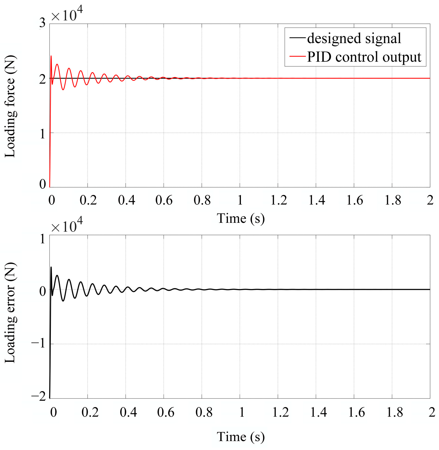
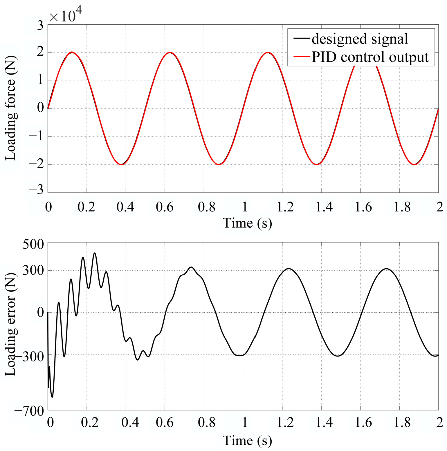
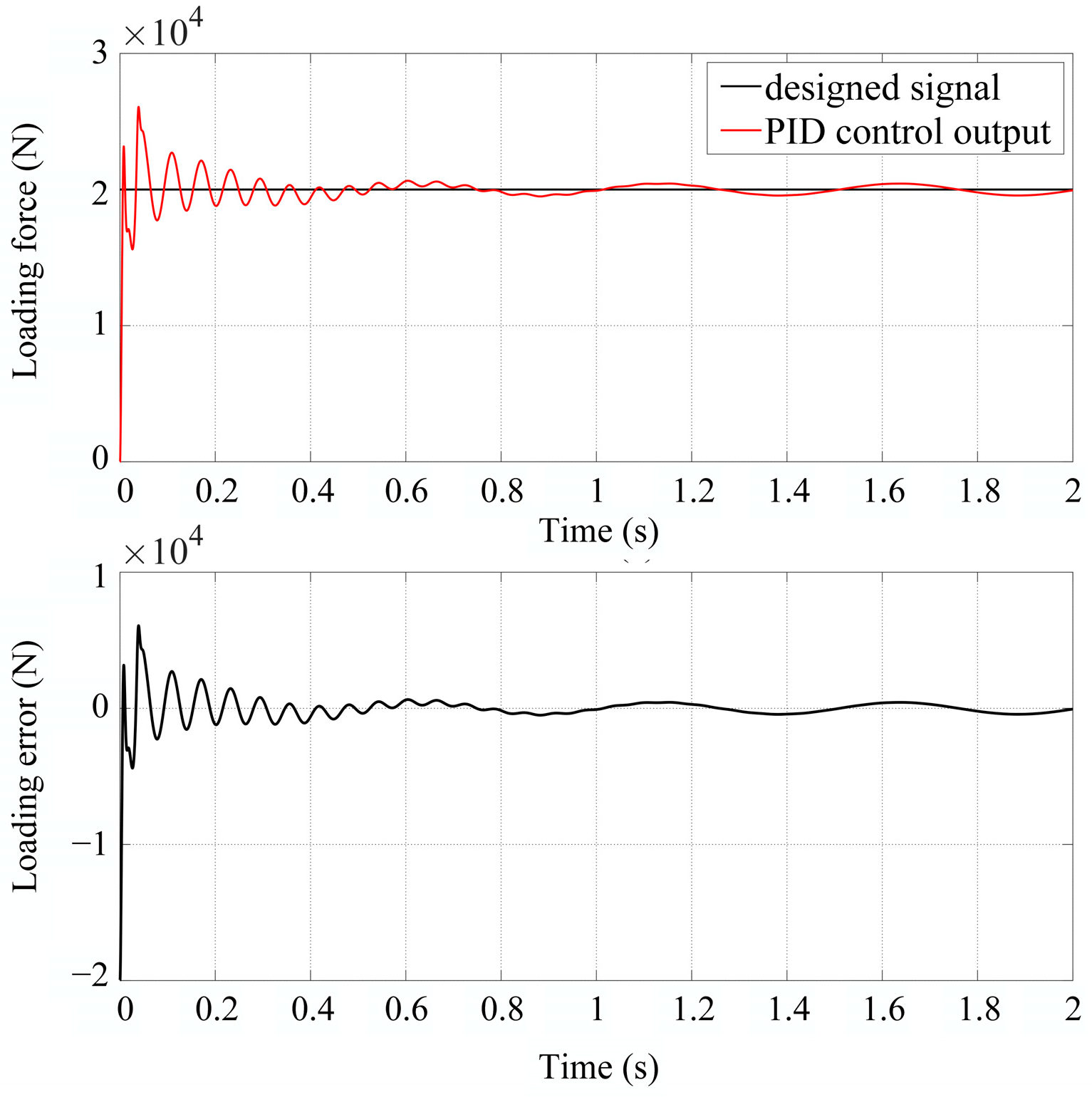
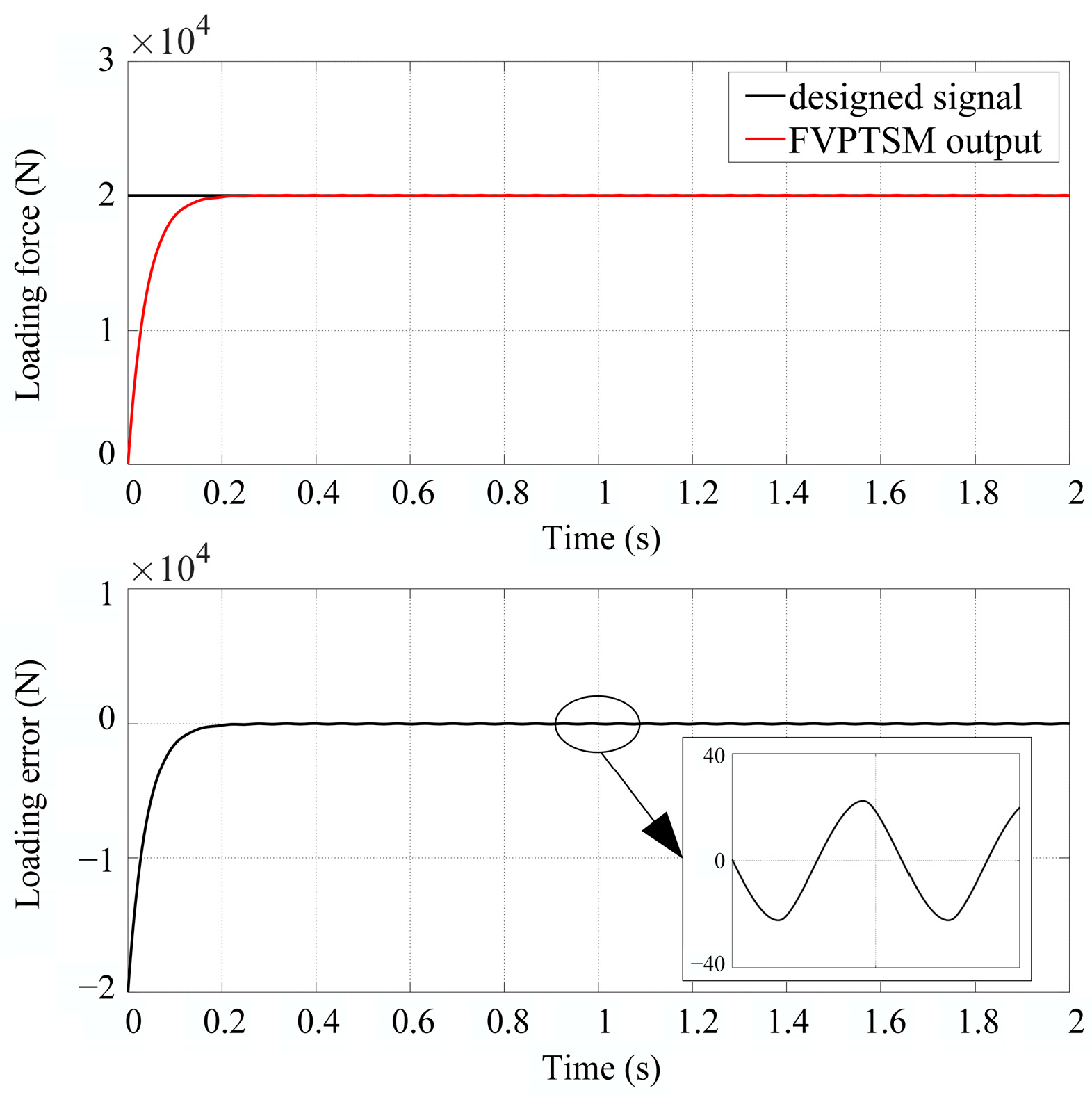
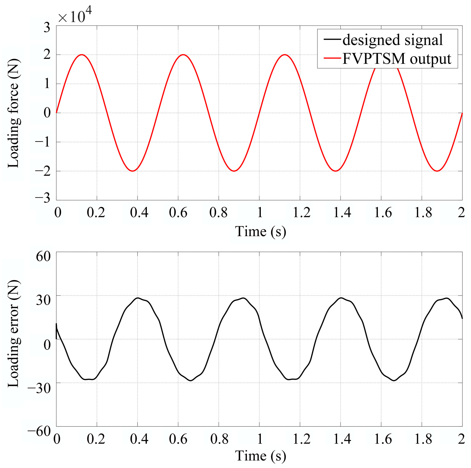
4.1. Simulation Verification

To validate the effectiveness and superiority of the aforementioned control strategies, simulations and analyses are conducted on the PID, DPTSM, and FVPTSM control strategies under both disturbed and undisturbed conditions. Meanwhile, a comparative analysis is performed to evaluate their respective control effects. Firstly, under interference-free conditions, a simulation comparison of the three control strategies is adopted to assess their force-tracking accuracy and the rapidity of the system response, aiming to determine whether the performance meets requirements. Additionally, the anti-interference performance and effectiveness of the FVPTSM controller are demonstrated by simulation comparison under the influence of disturbances. The simulation conditions are listed in

Table 1. Simulation conditions of electro-hydraulic load simulator.

Signal Type	Amplitude	Frequency (Hz)
Step loading signal	20,000 N	-
Sine loading signal	20,000 N	2
Sine position disturbance	30 mm	2

.

As shown in Figure 5, the difference between the force feedback from the electro-hydraulic loading simulator and the loading signal is utilized as the error function. The input signal corresponds to the loading instruction, while accounting for positional disturbances in the tested servo actuator. The step and sinusoidal signal simulations of the PID controller are conducted under two conditions: without actuator disturbance and with actuator disturbance. This enables the generation of output force and loading error data from the electro-hydraulic loading simulator, thereby evaluating the system’s force-tracking performance and anti-interference capability under controller influence. The swarm intelligence method [38] is adopted in the tuning of the PID parameters, and the optimal control gains are $K_{\mathrm{P}}=0.0015$, $K_{\mathrm{I}}=0.015$, and $K_{\mathrm{D}}=0$ without actuator disturbance and $K_{\mathrm{P}}=0.0004$, $K_{\mathrm{I}}=0.001$, and $K_{\mathrm{D}}=0$ with actuator disturbance. From the simulation results illustrated in Figure 6, Figure 7, Figure 8 and Figure 9, it is observed that under undisturbed loading conditions, the PID controller ensures a certain response speed and steady-state control accuracy; however, it exhibits significant oscillation and overshoot during step loading, as well as a phase lag phenomenon during sinusoidal loading. Under disturbed loading conditions, there is even an greater overshoot and phase lag compared to those in an undisturbed loading, which significantly impacts the tracking accuracy of the load spectrum in the electro-hydraulic loading simulator.

According to the sliding mode controller of the derived double-power reaching law, the controller model is constructed and integrated into the simulation model of the electro-hydraulic loading simulator, as depicted in Figure 10. As shown in Figure 11, Figure 12, Figure 13 and Figure 14, under undisturbed loading conditions, the steady-state error of the step response is effectively eliminated, resulting in a system with zero overshoot. The phase lag of the sine response is significantly reduced, leading to an error peak of 12 N. In the presence of disturbance loading, the steady-state error peak for the step response reaches approximately 47.1 N, while maintaining the absence of overshoot behavior. Similarly, the sine response exhibits a peak error of 50.3 N.

According to the FVPTSM derived from the design, it is incorporated into the sliding mode controller. Subsequently, loading simulations are conducted under two conditions—no actuator disturbance and actuator disturbance—as shown in Figure 10, analyzing the effectiveness and superiority of the proposed controller. Under undisturbed loading conditions, as illustrated in Figure 15 and Figure 16, the step response exhibits a virtually eliminated steady-state error with no overshoot observed in the system’s behavior. Additionally, a significant reduction in phase lag is achieved for the sine responses, resulting in an error peak of 12 N. From Figure 17 and Figure 18, it is observed that a steady-state error peak of approximately 22.6 N is observed in the step response, while maintaining a zero overshoot within the system’s dynamics under disturbed loading conditions. Furthermore, a peak error of 28.3 N is recorded for the sine responses.

As depicted in Figure 19, under step loading without actuator position disturbance, the PID controller, DPTSM, and FVPTSM exhibit a zero steady-state error, with no significant difference observed in their control effects based on the two reaching laws. However, the PID controller exhibits a large overshoot and oscillation, with a slow convergence time, whereas the sliding mode controller demonstrates no overshoot, a fast convergence speed, and a higher loading accuracy. As shown in Figure 20, for sinusoidal loading without actuator disturbance, both the DPTSM and FVPTSM yield similar control effects. As compared to the PID controller, sliding mode controllers based on the two reaching laws significantly reduce the loading error, while eliminating high-frequency oscillations from the error curve.

From the comparison of the simulation results in Figure 21 and Figure 22, a noticeable increase is demonstrated in the loading error of the PID controller when subjected to disturbance loading. This result is primarily due to the surplus force generated by position disturbances, resulting in an inadequate suppression of the excess forces. In contrast, the sliding mode controller exhibits a significantly improved force-loading accuracy compared to the PID controller. Furthermore, the FVPTSM outperforms the DPTSM in terms of force-loading accuracy and offers a superior suppression of excess forces.

The analysis of the aforementioned results reveals that the proposed sliding mode controller exhibits a significantly superior excess force suppression effect compared to the traditional PID controller. Moreover, in the presence of disturbances, the FVPTSM outperforms the DPTSM in terms of excess force suppression.

4.2. Experimental Verification

The experimental verification of the proposed controller is essential to demonstrate its effectiveness. The 3D model, test rig, and hydraulic schematic, as shown in Figure 23 and Figure 24, incorporate a double-rod symmetrical hydraulic cylinder controlled by a servo valve for force loading, while a servo electric cylinder is employed to simulate the position disturbance experienced by the actual tested servo actuator. Moreover, closed-loop control is achieved through feedback from the force sensor. The specifications of the key components adopted in the test rig are listed in

Table 2. Specification of key components in simulator test rig.

Signal Type	Amplitude	Frequency (Hz)
Hydraulic supply	Customized	System pressure: 25 MPa Max flow rate: 40 L/min
Loading hydraulic cylinder	SFG-50-36-260	Rated pressure: 25 MPa Max output force: 50,000 N
Servo valve	D633-313B	Rated flow: 40 L/min
Force sensor	CYB-602S-5T	Range: 0~50,000 N Accuracy: 0.1% FS
Displacement sensor	Magnetostrictive displacement sensor	Range: 0~270 mm Accuracy: 0.005% FS
Data acquisition card	USB1902	Voltage acquisition channels: 16
Linear electric cylinder	FDR075	Stroke: ±50 mm Max output force: 10,000 N
Servo driver	SV-DA200	AC380V pulse I/O control

. The PID, DPTSM, and FVPTSM controllers are embedded in the host computer software. The step- and sine-command loading experiments are conducted under both disturbed and undisturbed conditions for comparative verification. The experimental conditions are listed in

Table 3. Experimental conditions of electro-hydraulic load simulator.

Signal Type	Amplitude	Frequency (Hz)
Step loading signal	3000 N	-
Sine loading signal	3000 N	0.05
Sine position disturbance	10 mm	0.4

.

As shown in Figure 25, both the PID controller and the sliding mode controllers of the two reaching laws ensure a smaller steady-state loading error for step instruction loading without interference. The loading accuracy of the two reaching laws is essentially equivalent. However, the PID controller exhibits a significant overshoot and a longer convergence time. As illustrated in Figure 26, for sinusoidal command loading with sine position disturbance, a similar loading accuracy with a reduced phase lag and loading error is demonstrated by the two sliding mode controllers, as compared to those by the PID controller. The experimental results for undisturbed loading are consistent with the simulation outcomes.

From the results of the step and sine response with sine position disturbance, as shown in Figure 27 and Figure 28, respectively, due to the influence of excess force, under the step command signal, the loading accuracy of the PID controller is significantly compromised, and the overshoot and oscillation are more pronounced. In contrast, both sliding mode controllers, with their respective reaching laws, achieve superior suppression effects on the excess force, ensuring a high loading accuracy without any overshoot. Furthermore, the FVPTSM controller demonstrates a slightly better loading accuracy than the DPTSM controller, while also displaying a shorter rising time and faster response speed. The PID controller exhibits a poorer suppression of excess force, a lower loading accuracy, and greater phase lag than that of the sliding mode controllers in response to sinusoidal command loading. Meanwhile, the force-tracking performance of the FVPTSM is slightly superior to the DPTSM, which is similar to the step loading condition.

5. Conclusions

In this work, a modified fast variable-power terminal sliding mode control strategy (FVPTSM) is proposed for overcoming the system’s strong phase lag and position disturbance, to achieve the accurate force-tracking performance of the large-load and high-inertia aerospace electro-hydraulic load simulator. According to the system characteristics analyzed by the precise mathematical model and state–space model built by the authors, the feasibility and applicability of the algorithm is verified for rapid force tracking and high robustness. Furthermore, the FVPTSM is adopted in the design of the system controller, combined with the state–space model, and the finite-time convergence and asymptotic stability of the system are validated utilizing the Lyapunov stability analysis and proof. Additionally, the simulation and experimental results demonstrate the effectiveness of the proposed control algorithm, as compared to the conventional PID and the designed DPTSM methods, ensuring superior dynamic performance and stronger anti-interference ability and meeting the system requirements completely.

References

1. Chengwen, W.; Zongxia, J.; Shuai, W.; Bihua, C. “Dual-Loop Control” of load simulator. In Proceedings of the IEEE 10th International Conference on Industrial Informatics, Beijing, China, 25–27 July 2012; IEEE: Piscataway, NJ, USA, 2012; pp. 530–535. [Google Scholar]
2. Truong, D.Q.; Ahn, K.K. Force control for hydraulic load simulator using self-tuning grey predictor—Fuzzy PID. Mechatronics 2009, 19, 233–246. [Google Scholar] [CrossRef]
3. Asl, R.M.; Hagh, Y.S.; Simani, S.; Handroos, H. Adaptive square-root unscented Kalman filter: An experimental study of hydraulic actuator state estimation. Mech. Syst. Signal Process. 2019, 132, 670–691. [Google Scholar]
4. Won, D.; Kim, W.; Tomizuka, M. Nonlinear control with high-gain extended state observer for position tracking of electro-hydraulic systems. IEEE/ASME Trans. Mechatron. 2020, 25, 2610–2621. [Google Scholar] [CrossRef]
5. Jiang, W.; Zhang, C.; Jia, P.; Yan, G.; Ma, R.; Chen, G.; Ai, C.; Zhang, T. A Study on the Electro-Hydraulic Coupling Characteristics of an Electro-Hydraulic Servo Pump Control System. Processes 2022, 10, 1539. [Google Scholar] [CrossRef]
6. Hao, J.J.; Zhao, K.D. A Design Method of Electro-Hydraulic Load Simulator based on Flexible spring connection. Chin. J. Mach. Tool Hydraul. 2001, 4, 59–106. [Google Scholar]
7. Li, J.; Kong, L.; Liang, H.; Li, W.; Aldosary, S. Enhancing Electro-Hydraulic Load Simulator Performance through Variable Arm Length and Particle Swarm-Optimized Controllers. Nanoelectron. Optoe. 2023, 18, 1085–1099. [Google Scholar] [CrossRef]
8. Hu, H.; Zhang, Q.; Fang, J.; Wang, T.; Wei, J. Practical adaptive robust tracking control of the dual-valve parallel electro-hydraulic servo system with reduced-order model. Trans. Inst. Meas. Contr. 2024, 46, 501–512. [Google Scholar] [CrossRef]
9. Jianming, C.; Biao, Z.; Yanliang, D. A study on performance of electro-hydraulic load simulator based on pressure servo valve. In Proceedings of the 2015 International Conference on Fluid Power and Mechatronics (FPM), Harbin, China, 5–7 August 2015; IEEE: Piscataway, NJ, USA, 2015; pp. 505–509. [Google Scholar]
10. Matsui, T.; Mochizuki, Y. Effect of positive angular velocity feedback on torque control of hydraulic actuator. Trans. Jpn. Soc. Mech. Eng. 2008, 57, 1604–1609. [Google Scholar] [CrossRef]
11. Jacazio, G.; Balossini, G. A Mechatronic Active Force Control System for Real Time Test Loading of an Aircraft Landing Gear. In Proceedings of the International Design Engineering Technical Conferences and Computers and Information in Engineering Conference, San Diego, CA, USA, 30 August–2 September 2009; pp. 11–18. [Google Scholar]
12. Phan, V.D.; Trinh, H.A.; Ahn, K.K. Backstepping Control of an Electro-Hydraulic Actuator using Kalman Filter. In Proceedings of the 2023 26th International Conference on Mechatronics Technology (ICMT), Busan, Republic of Korea, 18–21 October 2023; IEEE: Piscataway, NJ, USA, 2012; pp. 1–5. [Google Scholar]
13. Truong, H.V.A.; Nam, S.; Kim, S.; Kim, Y.; Chung, W.K. Backstepping-Sliding-Mode-Based Neural Network Control for Electro-Hydraulic Actuator Subject to Completely Unknown System Dynamics. IEEE Trans. Autom. Sci. Eng. 2023, 1–25. [Google Scholar] [CrossRef]
14. Naveen, C.; Meenakshipriya, B.; Sathiyavathi, S. Design and Implementation of Iterative Learning Control for an Electro-Hydraulic Servo System. J. Sci. Ind. Res. 2023, 82, 579–588. [Google Scholar]
15. Phan, V.D.; Ahn, K.K. Fault-tolerant control for an electro-hydraulic servo system with sensor fault compensation and disturbance rejection. Nonlinear Dynam. 2023, 111, 10131–10146. [Google Scholar] [CrossRef]
16. Nahian, S.A.; Dinh, T.Q.; Dao, H.V.; Ahn, K.K. An unknown input observer—EFIR combined estimator for electrohydraulic actuator in sensor fault-tolerant control application. IEEE/ASME Trans. Mechatron. 2020, 25, 2208–2219. [Google Scholar] [CrossRef]
17. Vyas, J.; Rengasamy, A.; Narayanan, L.S.; Gopalsamy, B. Theoretical and Experimental Investigation of Friction in Hydraulic Actuators. In Machines, Mechanism and Robotics, Proceedings of the iNaCoMM 2019, Mandi, Himachal Pradesh, India, 5–7 December 2019; Springer: Singapore, 2022; Volume 2, pp. 421–427. [Google Scholar] [CrossRef]
18. Zhang, W.; Ping, Z.; Fu, Y.; Zheng, S.; Zhang, P. Observer-Based Backstepping Adaptive Force Control of Electro-Mechanical Actuator with Improved LuGre Friction Model. Aerospace 2022, 9, 415. [Google Scholar] [CrossRef]
19. Kang, S.; Yan, H.; Dong, L.; Li, C. Finite-time adaptive sliding mode force control for electro-hydraulic load simulator based on improved GMS friction model. Mech. Syst. Signal Process. 2018, 102, 117–138. [Google Scholar] [CrossRef]
20. Min, H.K.; Sung, H.J.; Lee, J.H.; Park, M.K. Robust control of electro-hydraulic load simulator using sliding mode control with Perturbation Estimation. In Proceedings of the 2017 17th International Conference on Control, Automation and Systems (ICCAS), Jeju, Republic of Korea, 18–21 October 2017; IEEE: Piscataway, NJ, USA, 2017; pp. 1137–1141. [Google Scholar]
21. Nahian, S.A.; Truong, D.Q.; Chowdhury, P. Modeling and fault-tolerant control of an electro-hydraulic actuator. Int. J. Precis. Eng. Manuf. 2016, 17, 1285–1297. [Google Scholar] [CrossRef]
22. Huang, J.; Song, Z.; Wu, J.; Guo, H.; Qiu, C.; Tan, Q. Parameter Adaptive Sliding Mode Force Control for Aerospace Electro-Hydraulic Load Simulator. Aerospace 2023, 10, 160. [Google Scholar] [CrossRef]
23. Kang, S.; Nagamune, R.; Yan, H. Almost disturbance decoupling force control for the electro-hydraulic load simulator with mechanical backlash. Mech. Syst. Signal Process. 2020, 135, 106400. [Google Scholar] [CrossRef]
24. Yu, W.; Yu, X.; Wang, H. Sliding modes: From asymptoticity, to finite time and fixed time. Sci. China Inf. Sci. 2023, 66, 190205. [Google Scholar] [CrossRef]
25. Moulay, E.; Léchappé, V.; Bernuau, E.; Defoort, M.; Plestan, F. Fixed-time sliding mode control with mismatched disturbances. Automatica 2022, 136, 110009. [Google Scholar] [CrossRef]
26. Moulay, E.; Léchappé, V.; Bernuau, E.; Plestan, F. Robust fixed-time stability: Application to sliding-mode control. IEEE Trans. Autom. Control 2021, 67, 1061–1066. [Google Scholar] [CrossRef]
27. Yu, X.; Feng, Y.; Man, Z. Terminal sliding mode control—An overview. IEEE Open J. Ind. Electron. Soc. 2020, 2, 36–52. [Google Scholar] [CrossRef]
28. Yu, X.; Zhihong, M. Fast terminal sliding-mode control design for nonlinear dynamical systems. IEEE Trans. Circuits Syst. I Fundam. Theory Appl. 2002, 49, 261–264. [Google Scholar]
29. Tong, X.; Zhao, H.; Feng, G. Adaptive global terminal sliding mode control for anti-warship missiles. In Proceedings of the 2006 6th World Congress on Intelligent Control and Automation, Dalian, China, 21–23 June 2006; IEEE: Piscataway, NJ, USA, 2006; pp. 1962–1966. [Google Scholar]
30. Moghaddam, R.K.; Mohamadie, N.K. Fast terminal nonsingular sliding mode control of wave energy converters for maximum power absorption. Ocean Eng. 2023, 281, 114473. [Google Scholar] [CrossRef]
31. Kardehi Moghaddam, R.; Baratpoor, J. Fuzzy Adaptive Nonsingular Terminal Sliding Mode Control of a Miniature Helicopter. J. Aerosp. Infor. Syst. 2024, 21, 140–151. [Google Scholar] [CrossRef]
32. Alnufaie, L. Nonsingular fast terminal sliding mode controller for a robotic system: A fuzzy approach. Eng, Tech. Applied Sci. Research 2023, 13, 11667–11671. [Google Scholar] [CrossRef]
33. Dong, R.Q.; Qi, W.N.; Lyu, X. Singularity-Free Fixed-time Sliding Mode Control for A Class of Nonlinear Systems. Aerosp. Sci. Technol. 2024, 146, 108952. [Google Scholar] [CrossRef]
34. Kasera, S.; Kumar, A.; Prasad, L.B. Analysis of chattering free improved sliding mode control. In Proceedings of the 2017 International Conference on Innovations in Information, Embedded and Communication Systems (ICIIECS), Coimbatore, India, 17–18 March 2017; IEEE: Piscataway, NJ, USA, 2012; pp. 1–6. [Google Scholar]
35. Young, K.D.; Utkin, V.I.; Ozguner, U. A control engineer’s guide to sliding mode control. IEEE Trans. Control Syst. Technol. 1999, 7, 328–342. [Google Scholar] [CrossRef]
36. Liu, S.Q.; Whidborne, J.F.; zhi Lyv, W.; Zhang, Q. Observer based incremental backstepping terminal sliding-mode control with learning rate for a multi-vectored propeller airship. Aerosp. Sci. Technol. 2023, 140, 108490. [Google Scholar] [CrossRef]
37. Huang, S.; Jiang, J.; Li, O. Adaptive Neural Network-Based Sliding Mode Backstepping Control for Near-Space Morphing Vehicle. Aerospace 2023, 10, 891. [Google Scholar] [CrossRef]
38. Wati, D.A.R. Performance evaluation of swarm intelligence on model-based PID tuning. In Proceedings of the 2013 IEEE International Conference on Computational Intelligence and Cybernetics, (CYBERNETICSCOM), Yogyakarta, Indonesia, 3–4 December 2013; IEEE: Piscataway, NJ, USA, 2017; pp. 40–44. [Google Scholar]
Figure 1. Mechanical structure and construction of the aerospace electro-hydraulic load simulator.
Actuators 13 00145 g001
Figure 2. Schematic diagram of electro-hydraulic load simulator.
Actuators 13 00145 g002
Figure 3. Block diagram of open-loop transfer function of electro-hydraulic load simulator.
Actuators 13 00145 g003
Figure 4. The phase trajectory diagram of the system.
Actuators 13 00145 g004
Figure 5. Simulation schematic of PID controller for electro-hydraulic load simulator.
Actuators 13 00145 g005
Figure 6. Step response simulation of force-tracking performance under PID control without interference.
Actuators 13 00145 g006
Figure 7. Sine response simulation of force-tracking performance under PID control without interference.
Actuators 13 00145 g007
Figure 8. Step response simulation of force-tracking performance under PID control with sine position disturbance.
Actuators 13 00145 g008
Figure 9. Sine response simulation of force-tracking performance under PID control with sine position disturbance.
Actuators 13 00145 g009
Figure 10. Simulation schematic of SMC controller for electro-hydraulic load simulator.
Actuators 13 00145 g010
Figure 11. Step response simulation of force-tracking performance under DPTSM control without interference.
Actuators 13 00145 g011
Figure 12. Sine response simulation of force-tracking performance under DPTSM control without interference.
Actuators 13 00145 g012
Figure 13. Step response simulation of force-tracking performance under DPTSM control with sine position disturbance.
Actuators 13 00145 g013
Figure 14. Sine response simulation of force-tracking performance under DPTSM control with sine position disturbance.
Actuators 13 00145 g014
Figure 15. Step response simulation of force-tracking performance under FVPTSM control without interference.
Actuators 13 00145 g015
Figure 16. Sine response simulation of force-tracking performance under FVPTSM control without interference.
Actuators 13 00145 g016
Figure 17. Step response simulation of force-tracking performance under FVPTSM control with sine position disturbance.
Actuators 13 00145 g017
Figure 18. Sine response simulation of force-tracking performance under FVPTSM control with sine position disturbance.
Actuators 13 00145 g018
Figure 19. Step response simulation of force-tracking performance under different control strategies without interference.
Actuators 13 00145 g019
Figure 20. Sine response simulation of force-tracking performance under different control strategies without interference.
Actuators 13 00145 g020
Figure 21. Step response simulation of force-tracking performance under different control strategies with sine position disturbance.
Actuators 13 00145 g021
Figure 22. Sine response simulation of force-tracking performance under different control strategies with sine position disturbance.
Actuators 13 00145 g022
Figure 23. The 3D model and test rig of the electro-hydraulic load simulator.
Actuators 13 00145 g023
Figure 24. Hydraulic cylinder loading section and hydraulic schematic.
Actuators 13 00145 g024
Figure 25. Response curve of force-tracking performance of 3000 N step signal under different control strategies without interference.
Actuators 13 00145 g025
Figure 26. Response curve of force-tracking performance of 3000 N, 0.05 Hz sinusoidal signal under different control strategies without interference.
Actuators 13 00145 g026
Figure 27. Response curve of force-tracking performance of 3000 N step signal under different control strategies with 10 mm, 0.4 Hz sinusoidal position disturbance.
Actuators 13 00145 g027
Figure 28. Response curve of force-tracking performance of 3000 N, 0.05 Hz sinusoidal signal with 10 mm, 0.4 Hz sinusoidal position disturbance.
Actuators 13 00145 g028