
Design and Analysis of the Mechanical Structure of a Robot System for Cabin Docking


Abstract
:1. Introduction
- (1)
- Three-coordinate POGO column assembly: The three-coordinate POGO column structure is used to adjust the position and pose of the workpiece [1,2,3]. The POGO column is an adjustable support system with three orthogonal translation degrees of freedom, which is composed of three mutually orthogonal translation units, and can adjust the supported parts in space with high precision. Aiming at the aircraft wing assembly problem, a six-DOF attitude docking system based on a three-DOF POGO column was proposed [4]. Each positioner is connected to the wing by a hemispherical end effector. The positioner and the wing mechanism form a three-PPPS (P is a moving joint, S is a spherical joint) redundant drive variable mechanism. Assembly by the three-coordinate POGO column makes the production line have high flexibility. However, this assembly method has certain limitations; for example, the distributed POGO column is redundant in motion control, which will bring high difficulty and economic cost to the control.
- (2)
- Stewart platform assembly: The Stewart platform is used to adjust the position and pose of the workpiece. A Stewart platform refers to a symmetrical parallel mechanism with six degrees of freedom [5,6]. Based on the six-SPS parallel mechanism, which is used to adjust the attitude of the module [7], a force sensor is integrated in each sliver chain of the parallel mechanism to achieve flexible docking control of the module through force feedback, so as to reduce the risk of damaged parts. Compared with distributed POGO columns, the Stewart platform is more compact and easier to control. However, this assembly method has certain limitations for the assembly of cabin parts with different diameters and lengths, and it is not suitable for continuous production in the engineering environment.
- (3)
- Vertical assembly method: The components of the cabin are assembled vertically by means of lifting assembly. In the automatic docking of a satellite, a six-SPS parallel mechanism is used as the docking equipment to support the mobile module, and the mechanism can dock the mobile module with the suspended fixed module by adjusting its posture in the vertical direction [8]. However, the vertical assembly method requires enough space to be utilized in the vertical direction of the workshop, allowing multiple compartments to be placed vertically, which is not conducive to popularization and application in the general assembly workshop. At the same time, with an increase in the weight and size of the cabin, the vertical assembly method will become difficult to implement because of the difficulty of operation, high-risk factor, and increase in vertical assembly control.
- (4)
- Horizontal docking method: By lifting or AGV transfer, the cabin components are transferred to the attitude adjustment mechanism of the assembly workstation. The attitude adjustment mechanism can move horizontally along the guide rail to complete the assembly and docking of the multi-stage cabins. Aiming at the docking problem of a certain type of rocket module, the automatic docking platform of the rocket module was built by the Shenyang Institute of Automation [9]. The six-DOF pose adjustment mechanism loaded with ring tooling is used as the pose adjustment platform of the docking module, and the transfer drive and the docking drive of the module are designed in an integrated way. Aiming to address the high precision and automation requirements of spacecraft module docking assembly, the Beijing Institute of Satellite Environmental Engineering proposed large module horizontal docking assembly technology based on automation means [10] and designed the module horizontal docking system structure.
2. Functional Requirements and Key Indicators of the Module Docking Robot
2.1. Functional Requirements of the Cabin Docking Robot
- (1)
- Carrying a large load and large sized workpieces, and carrying weight not less than 500 kg;
- (2)
- High precision, reliable and stable motion function;
- (3)
- A certain product compatibility function that adapt to the compatibility function of different loads within a certain specification range.
2.2. Technical Indicators
- (1)
- Load capacity: including the motion accuracy of the robot platform, the degree of freedom of the robot, the load capacity of the robot, etc. These indicators determine the ability of the robot to perform the final task;
- (2)
- Working space: the robot must have the working range required for the assembly of cabin workpieces;
- (3)
- Motion speed: when the docking robot performs the assembly task, the docking robot is required to operate quickly and work efficiently.
3. Mechanical Design and Strength Analysis of the Cabin Docking Robot System
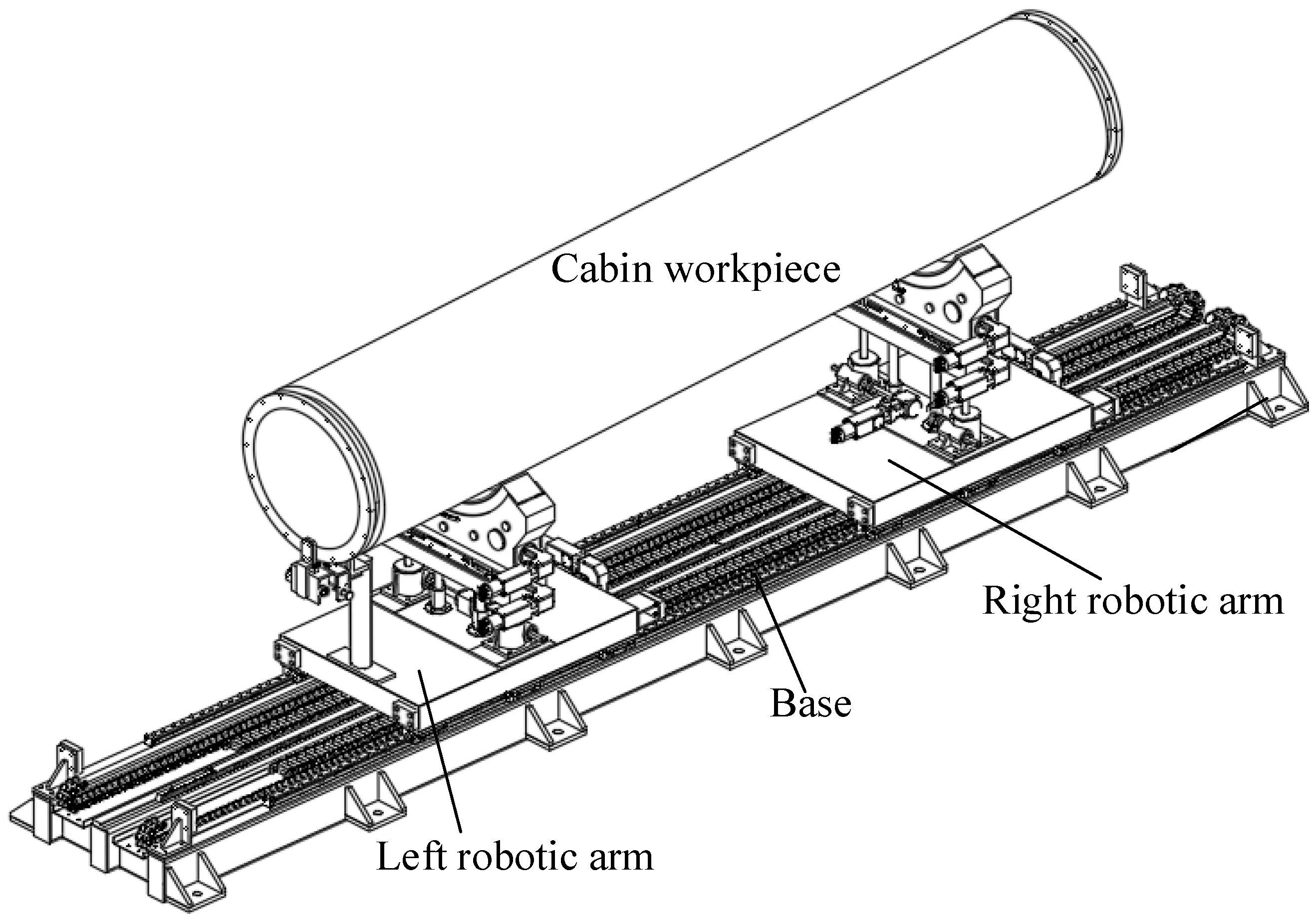
3.1. Overall Scheme of the Cabin Docking Robot System
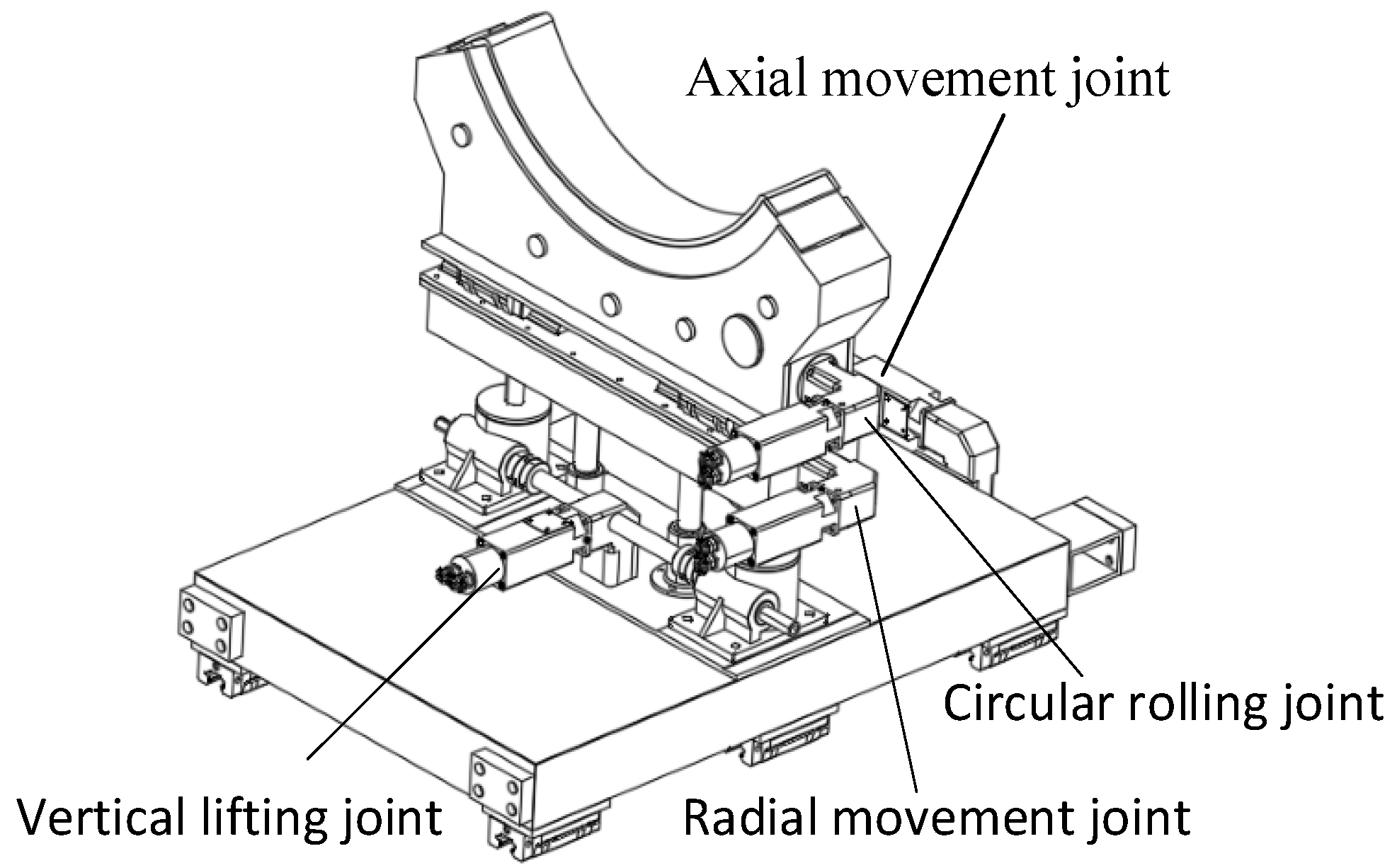
3.2. Joint Design of the Docking Robot
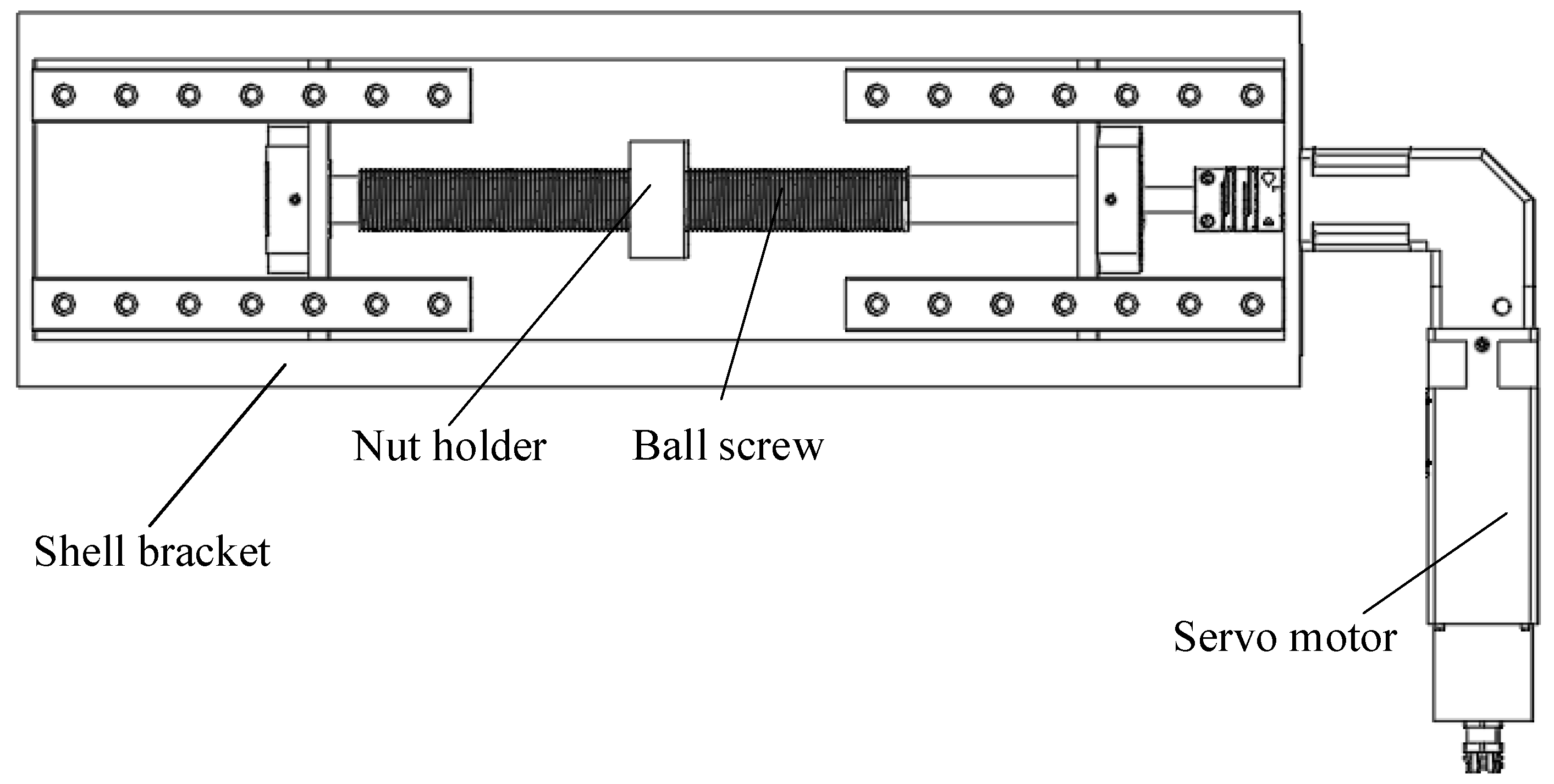
3.2.1. Axial Movement Joint
3.2.2. Vertical Lifting Joint
3.2.3. Radial Movement Joint
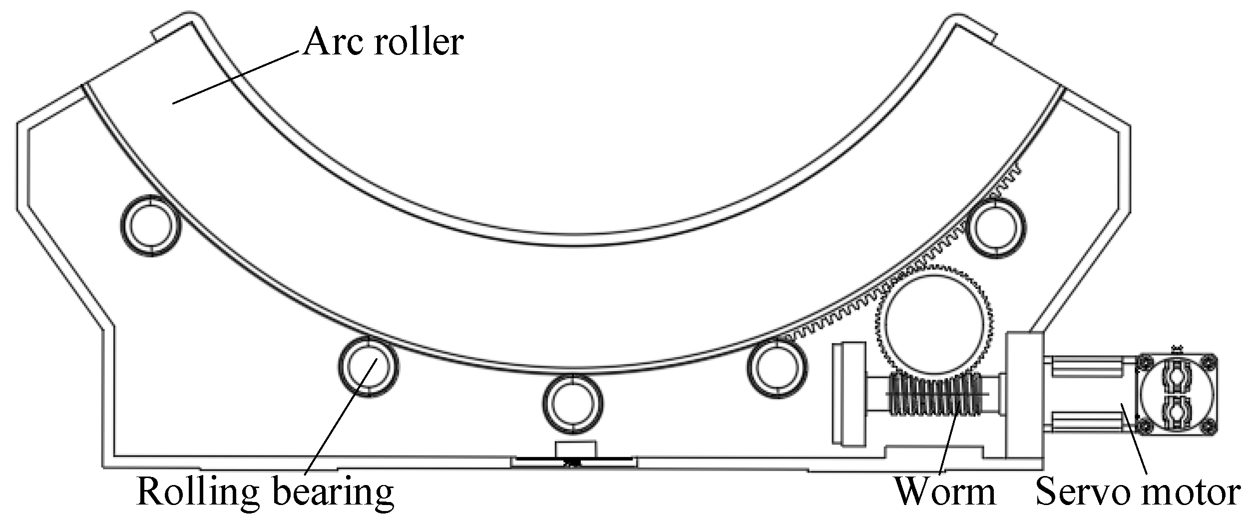
3.2.4. Circular Rolling Joint
3.3. Strength Analysis of Key Components
3.3.1. Strength Analysis of the Bottom Frame
3.3.2. Strength Analysis of the Spiral Elevator
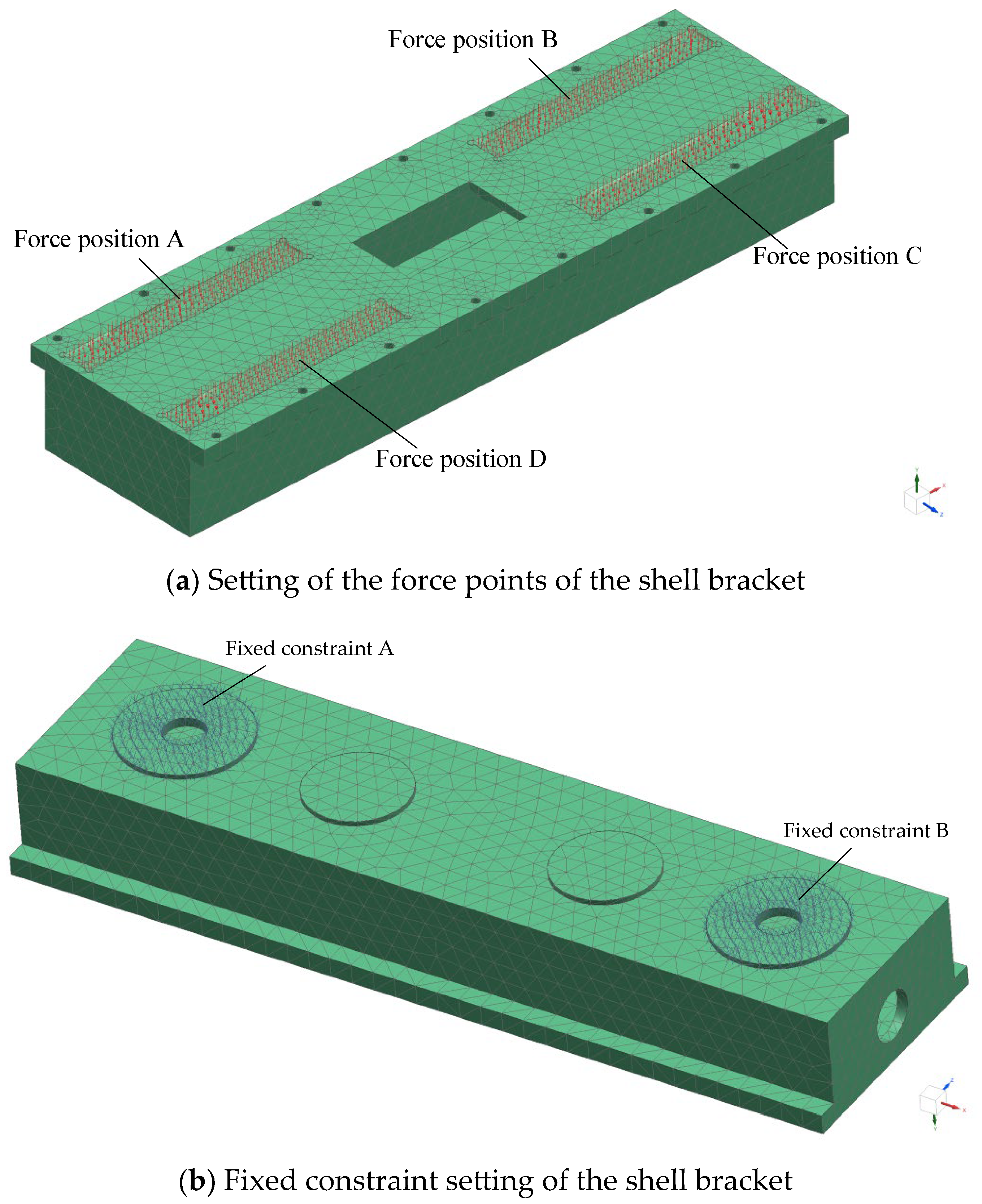
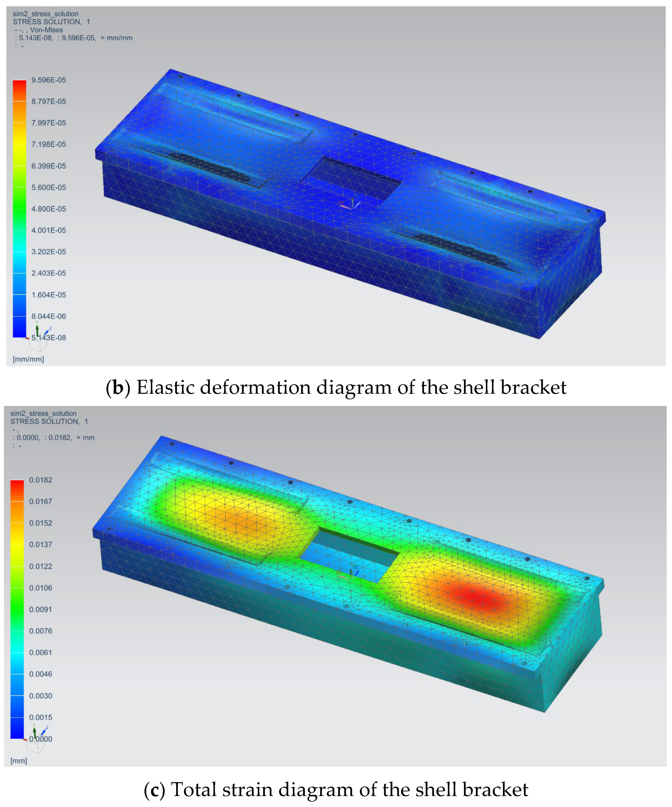
3.3.3. Strength Analysis of the Shell Bracket
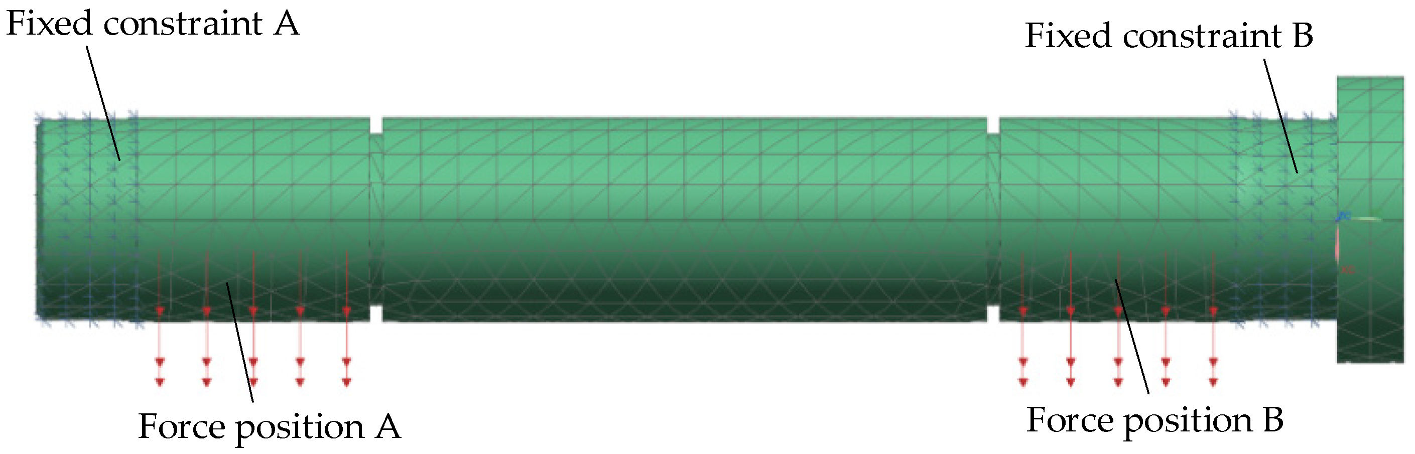
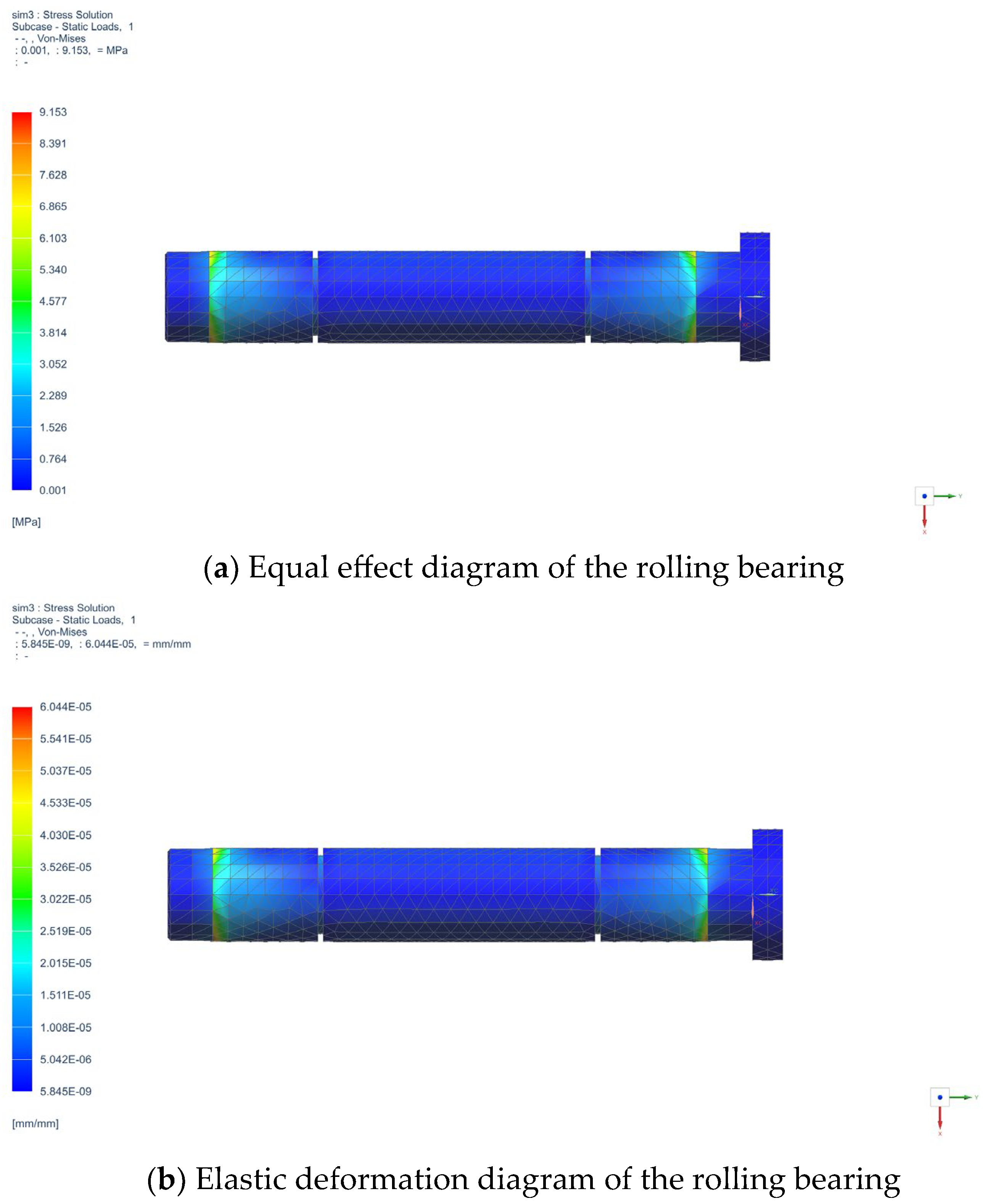
3.3.4. Strength Analysis of the Rolling Bearing
4. Kinematics Modeling and Simulation Verification
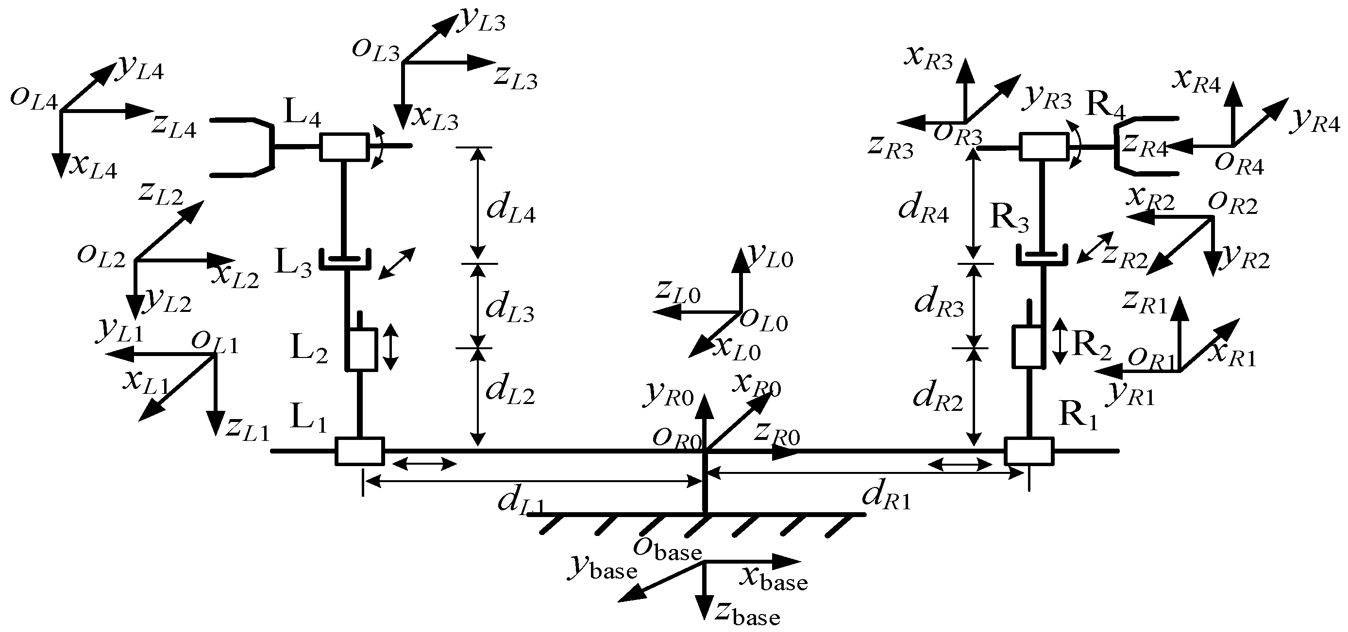
4.1. Kinematics Modeling
4.1.1. Kinematics Modeling of the Cabin Docking Robot System
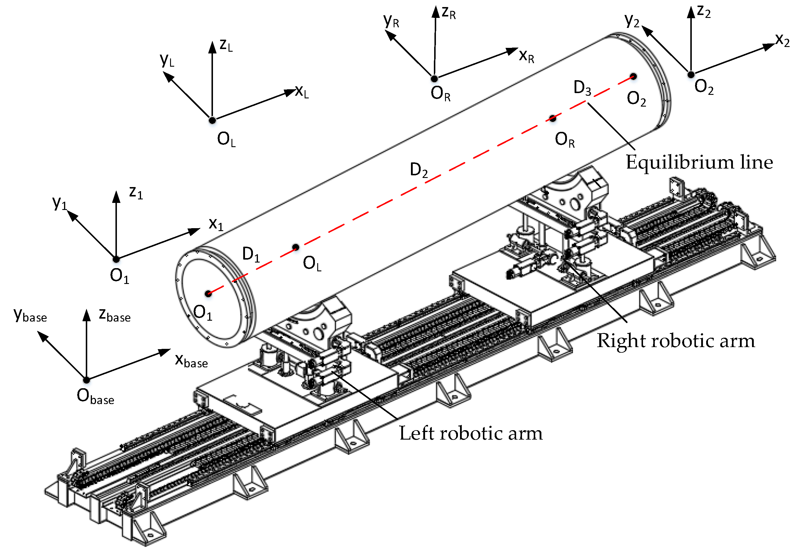
4.1.2. Joint Kinematics Modeling of the Cabin Docking Robot and Cabin Workpiece
- (1)
- Initial equilibrium position
- (2)
- The pitch angle of the cabin workpiece is not 0°
- (3)
- The yaw angle of the cabin workpiece is not 0°
- (4)
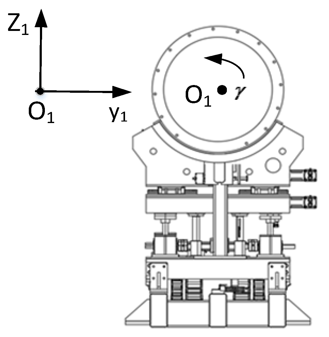
- The rolling angle of the cabin workpiece γ is not 0°
- (1)
- When the attitude of the module changes, the relative distance between the origin of the coordinate system at the end of the left robotic arm of the module docking and the origin of the coordinate system at the end of the right robotic arm of the module docking remains unchanged.
- (2)
- When the cabin roll angle changes, the position adjustment of the cabin docking robot is not affected, but the attitude of the cabin itself is affected.
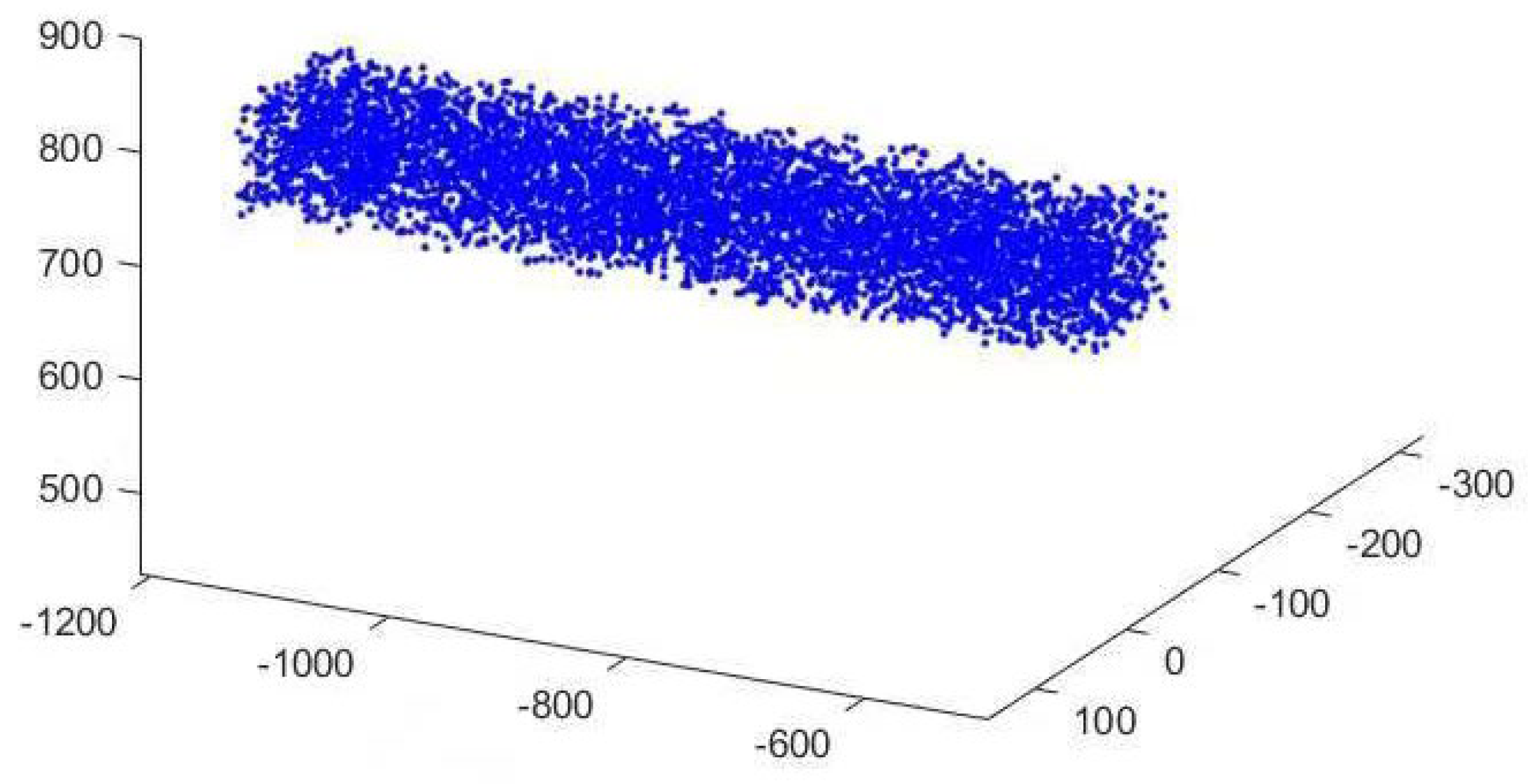
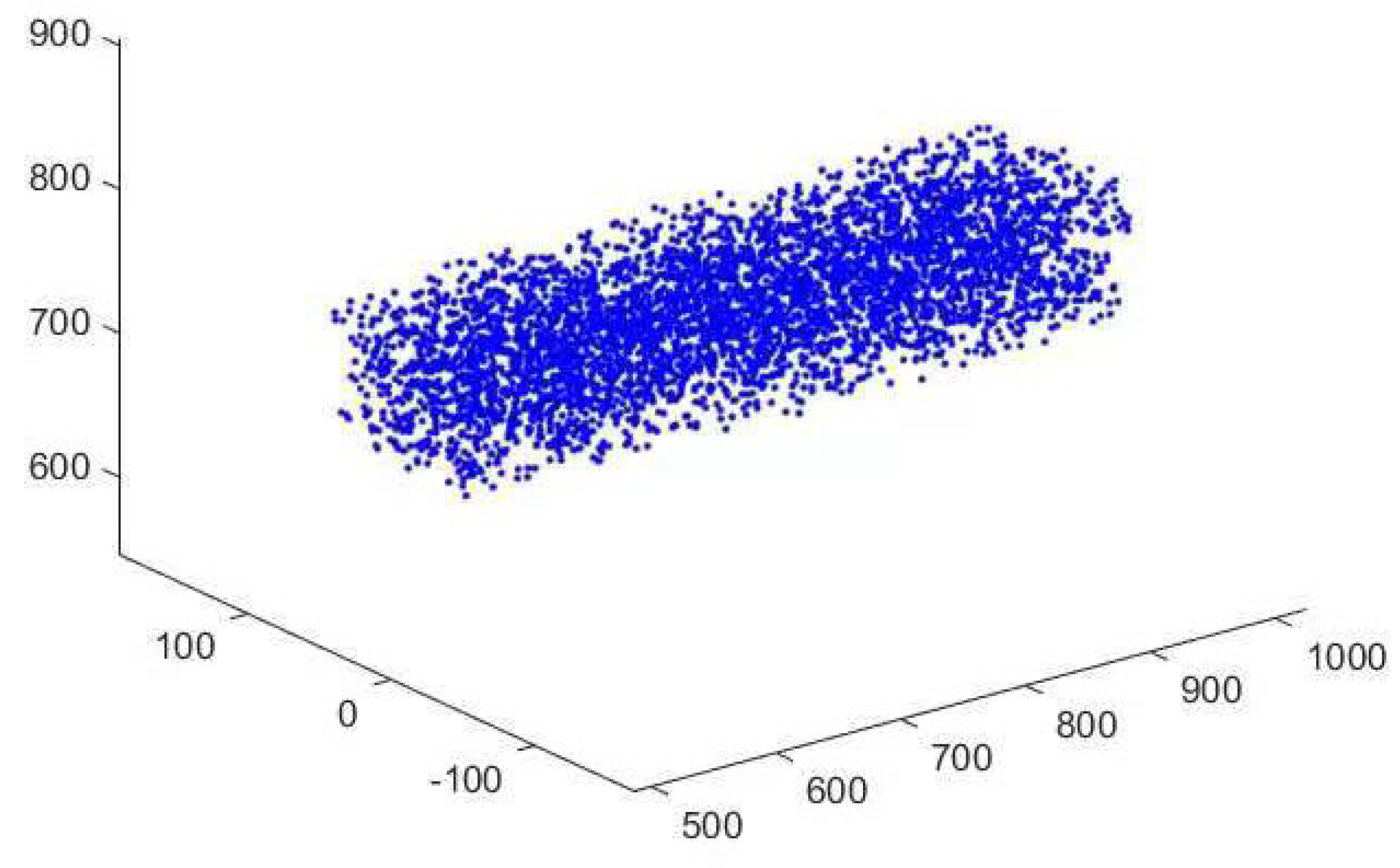
4.2. Workspace Analysis
- (1)
- Construct a probability model. In this paper, the probability distribution of the equivalent strain of the independent variable follows the normal distribution model.
- (2)
- Obtain sub-samples by simulation. Random numbers are generated within the constraints of each joint in the workspace according to the normal distribution, and the position in the operation space is obtained through the coordinate transformation relationship.
4.3. Kinematics Simulation
4.3.1. Kinematics Simulation of Cabin Docking Robot System
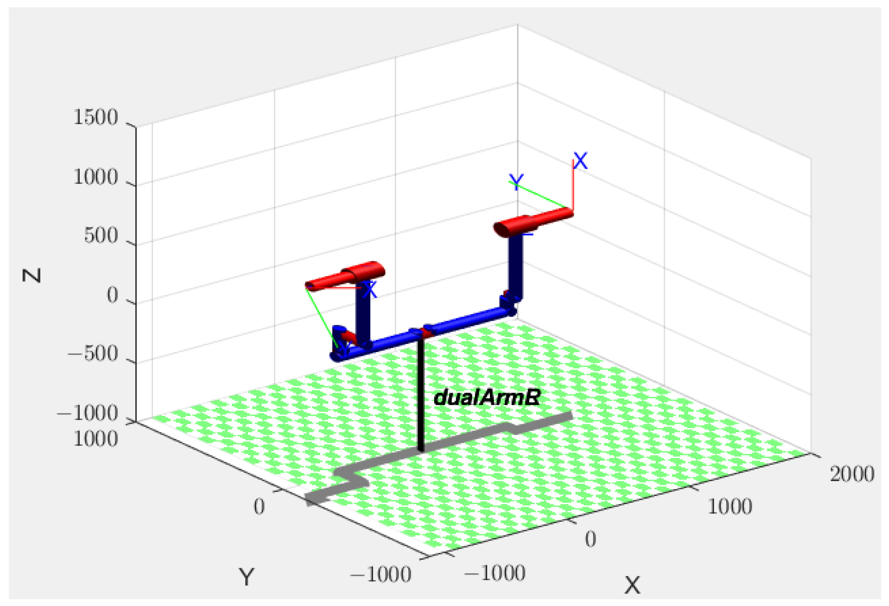
- (1)
- Establishment of simulation model
- (2)
- Kinematics simulation
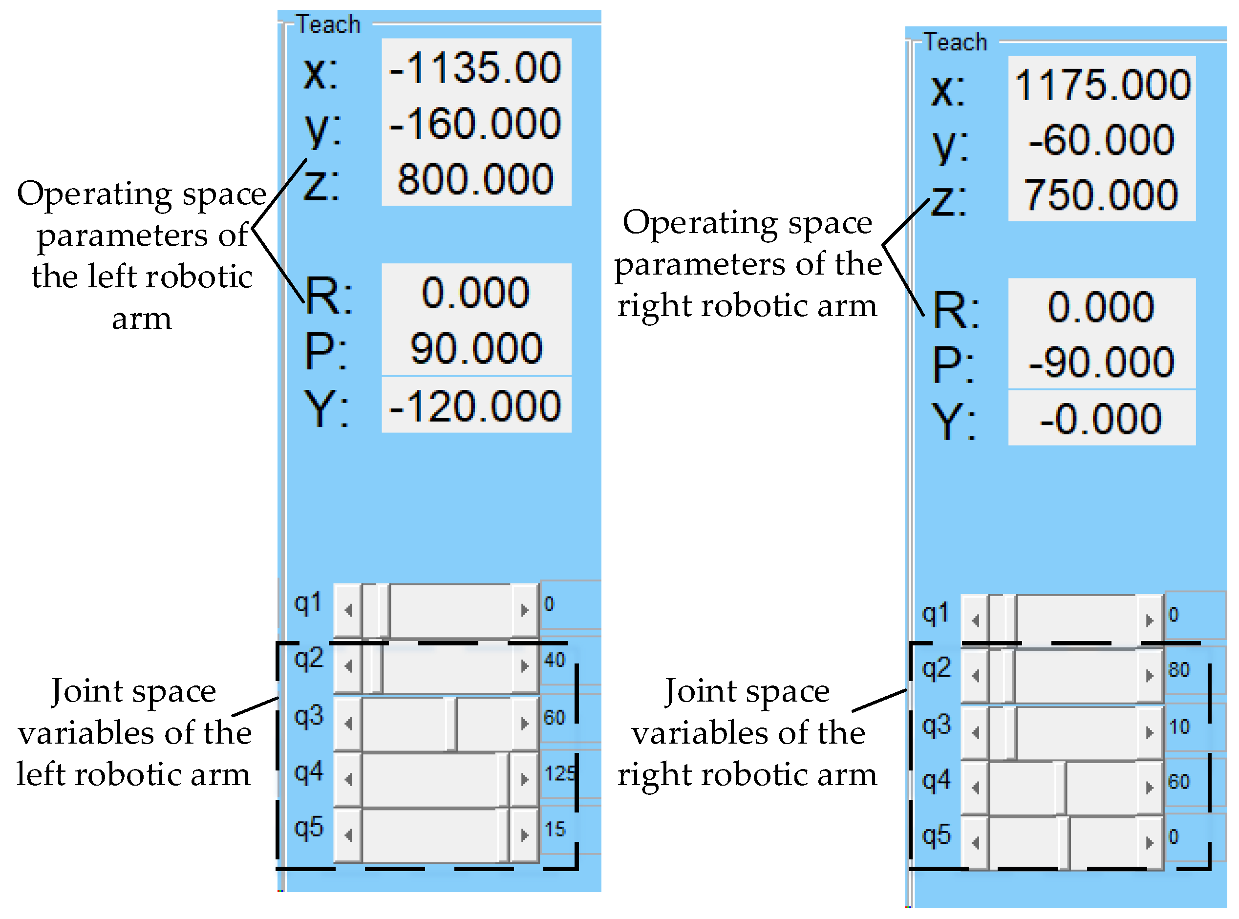
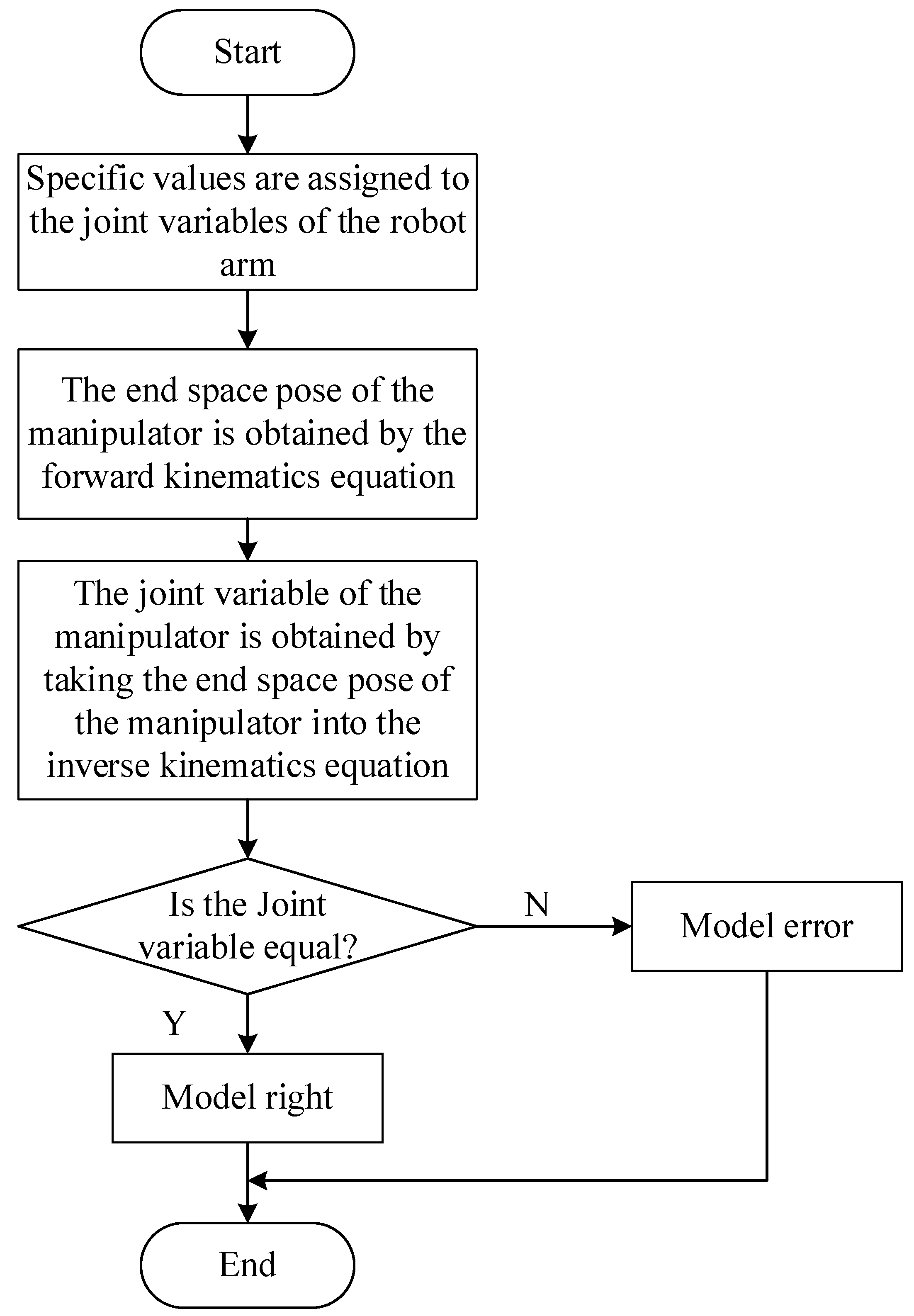
- (1)
- The joint variable of the left robotic arm is , and the joint variable of the right robotic arm is ;
- (2)
- Through forward kinematics calculation, the end space pose of the left robotic arm is , and the end space pose of the right robotic arm is ;
- (3)
- The space pose of the end of the robot arm is brought into the inverse kinematics equation, and the calculated joint space variable of the left robot arm is , and the joint variable of the right robot arm is ;
- (4)
- The inverse kinematics solution results in the joint variable being equal to the initial assignment, which proves that the kinematics model is correct.
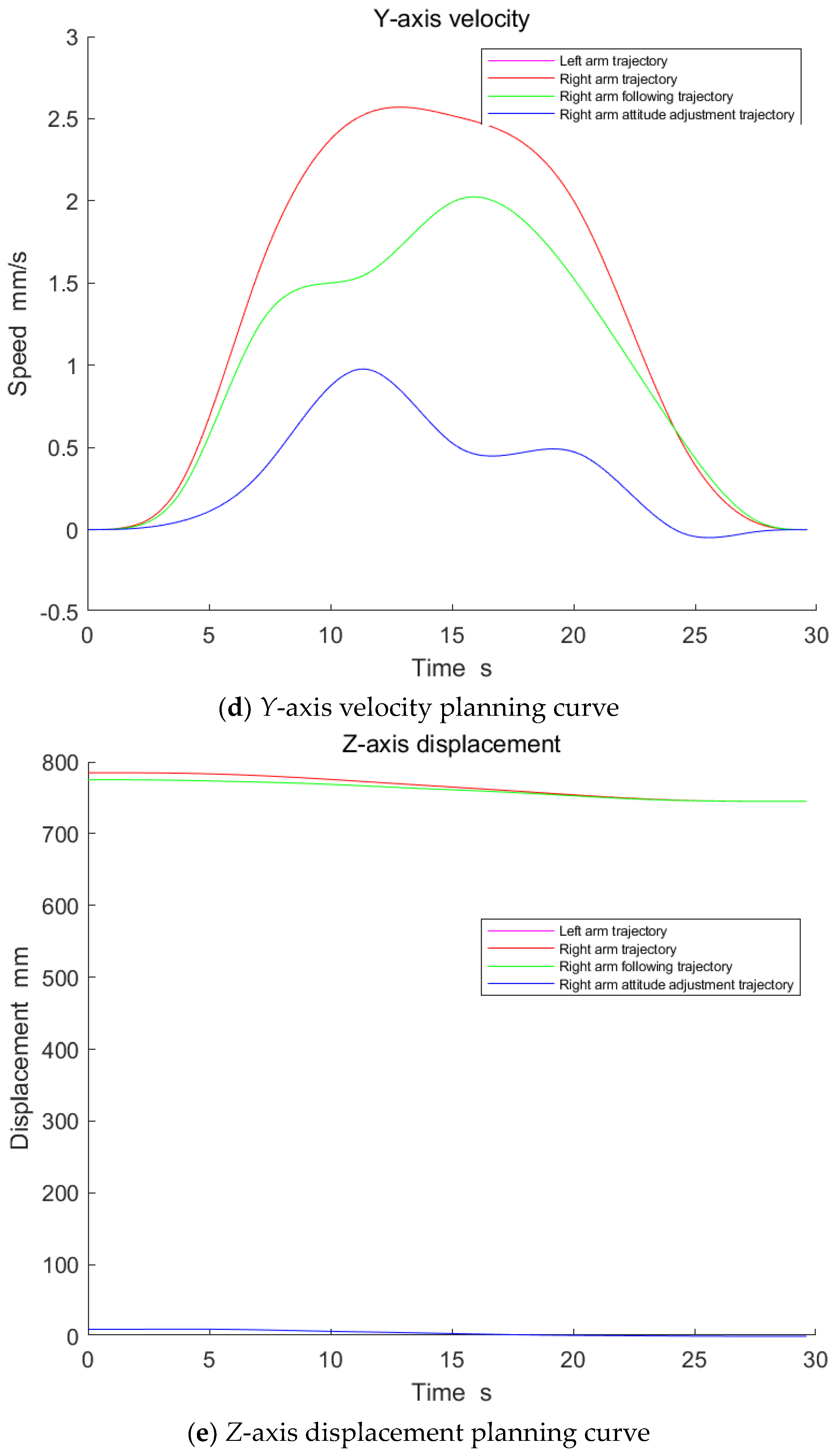
4.3.2. Joint Kinematics Simulation of the Cabin Docking Robot and Cabin Workpiece
- (1)
- Simulation parameter setting
- (2)
- Results of joint kinematics simulation
5. Experimental Verification
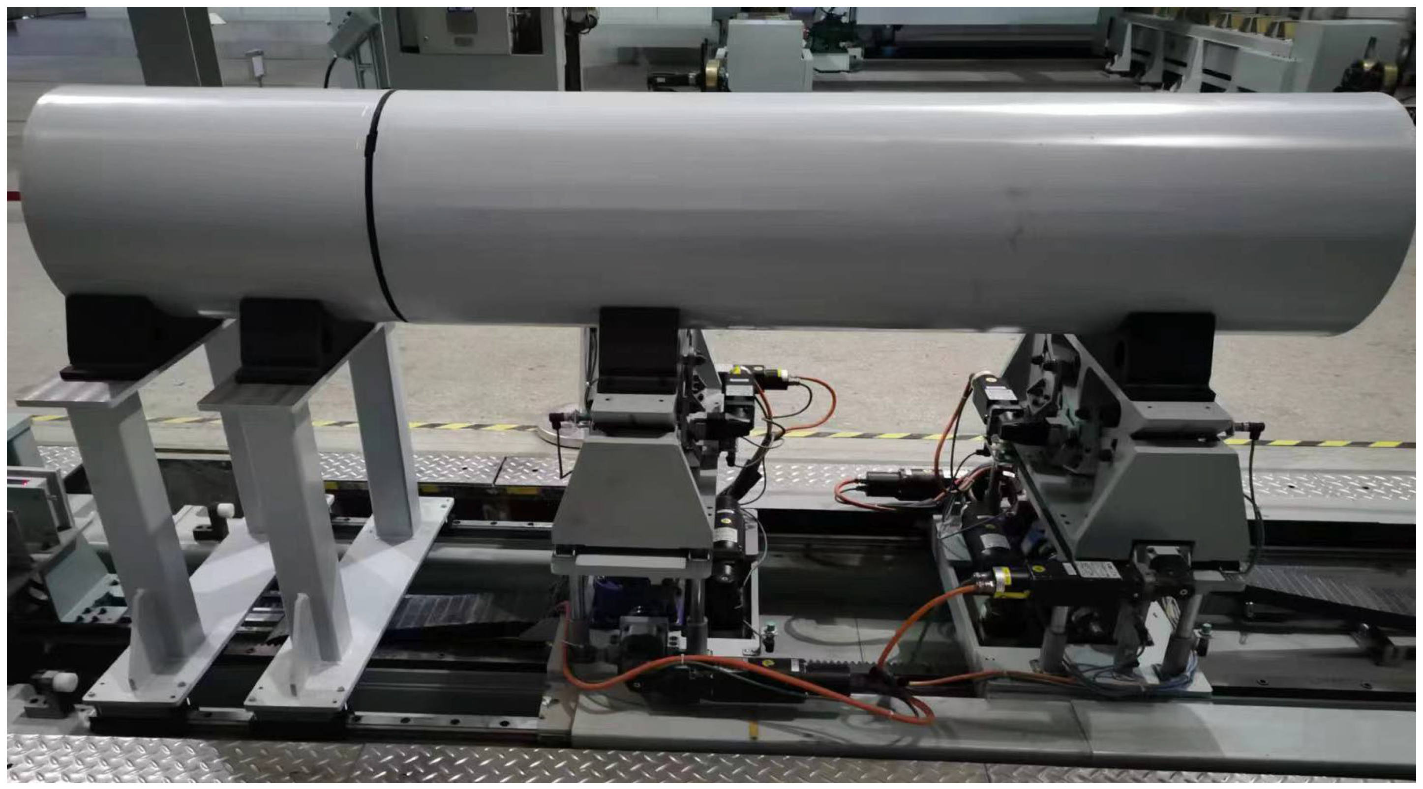
5.1. Development of a Prototype Robot System for Cabin Docking
5.2. Workspace Test Experiment
5.2.1. Experimental Methods
5.2.2. Experimental Results
5.3. Repeated Joint Positioning Accuracy Test
5.3.1. Experimental Methods
5.3.2. Experimental Results
5.4. Precision Experiment of Joint Motion Control
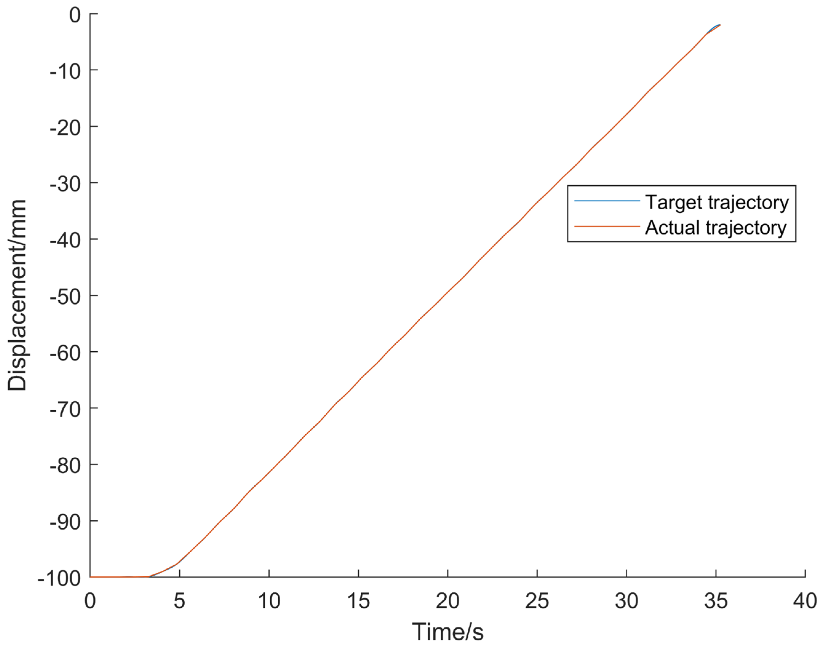
5.4.1. Control Accuracy of the Axial Movement Joint
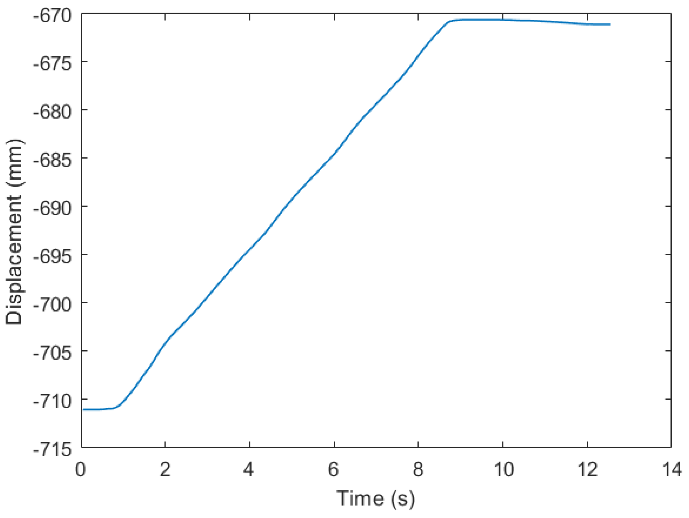
5.4.2. Control Accuracy of Vertical Lifting Joint
5.4.3. Control Accuracy of the Radial Movement Joint
5.4.4. Control Accuracy of the Circular Rolling Joint
5.5. Cabin Docking Experiment
5.6. Comparison of Robot Performance Indicators
6. Conclusions
- (1)
- The cabin docking robot is designed by the horizontal docking mode, and the composition and working principle of each joint of the robot are analyzed. The degree of freedom of the cabin docking robot is six, and the maximum load capacity can reach 1000 kg.
- (2)
- The static stress analysis of the key components of the robot joints is carried out by finite element software. The maximum equivalent stress of the bottom frame is 31.81 Mpa and the maximum total deformation is 0.125 mm. The maximum equivalent stress of the trapezoidal lead screw is 28.86 Mpa, and the maximum total deformation is 0.0177 mm. The maximum equivalent stress of the shell bracket is 23.13 Mpa, and the maximum total deformation is 0.0182 mm. The maximum equivalent stress of the rolling bearing is 9.153 Mpa, and the maximum total deformation is 0.001195 mm. The simulation results are all within the reasonable range.
- (3)
- The kinematics model of the robot is established based on the D-H modeling method, the forward and inverse kinematics relationship of the robot are analyzed, and the correctness of the kinematics model of the robot is verified by simulation.
- (4)
- The cabin docking robot and the joint kinematics model of the module are established and the correctness of the joint kinematics model is verified through simulation.
- (5)
- The working space, repeated positioning accuracy, and motion control accuracy of each joint of the robot are verified through experiments, which proved the effectiveness of the robot design.
Author Contributions
Funding
Data Availability Statement
Conflicts of Interest
References
- Guo, Z.M.; Jiang, J.X.; Ke, Y.L. Posture Alignment for Large Aircraft Parts Based on Three POGO Sticks Distributed Support. Acta Aeronaut. Astronaut. Sin. 2009, 30, 1319–1324. [Google Scholar]
- Guo, Z.M.; Jiang, J.X.; Ke, Y.L. Design and accuracy for POGO stick with three-axis. J. Zhejiang Univ. (Eng. Sci.) 2009, 43, 1649–1654. [Google Scholar]
- Jiang, J.X.; Chen, Q.; Fang, Q.; Ke, Y. Analysis and experimental test on dynamic characteristic of 3-axis positioner system. Comput. Integr. Manuf. Syst. 2009, 19, 1004–1009. [Google Scholar]
- Zhang, B.; Yao, B.; Ke, Y. A novel posture alignment system for aircraft wing assembly. J. Zhejiang Univ. Sci. A 2009, 10, 1624–1630. [Google Scholar] [CrossRef]
- Yuan, X.; Tang, Y.; Wang, W.; Zhang, L. Parametric Vibration Analysis of a Six-Degree-of-Freedom Electro-Hydraulic Stewart Platform. Shock. Vib. 2021, 2021, 1–27. [Google Scholar] [CrossRef]
- Jin, H.R.; Liu, D. Two-point Positioning and Pose Adjustment Method for Automatic Assembly of Barrel-type Cabin. China Mech. Eng. 2018, 29, 1467–1474. [Google Scholar]
- Dai, W.B.; Hu, R.Q.; Yi, W.M. The flexible docking technology for large spacecraft cabins. Spacecr. Environ. Eng. 2014, 31, 584–588. [Google Scholar] [CrossRef]
- Xiong, T. Automatic Docking Technology of Satellite. Aeronaut. Manuf. Technol. 2011, 22, 36–39. [Google Scholar] [CrossRef]
- Wang, B.X.; Xu, Z.G.; Wang, J.Y.; Wang, Y.J. Design and Research of Missile General Assembly Automatic Docking Platform. Mod. Def. Technol. 2016, 44, 135–141+147. [Google Scholar]
- Yi, W.M.; Duan, B.W.; Gao, F.; Han, X.G. Level docking technology in large cabin assembly. Comput. Integr. Manuf. Syst. 2015, 21, 2354–2360. [Google Scholar] [CrossRef]
- Guo, J.; Zhang, X.; Li, H.; Sun, X. Mechanism Design and Strength Analysis of Key Components of Flight-climbing-slide Robot for High-voltage Transmission Line Inspection. In Proceedings of the 2017 IEEE 7th Annual International Conference on CYBER Technology in Automation, Control, and Intelligent Systems (CYBER), Honolulu, HI, USA, 1 July–4 August 2017. [Google Scholar]
- Pao, J.C.; Banglos, C.A.; Salaan, C.J.; Guirnaldo, S.A. Simulation and Strength Analysis of Flippable Mobile Ground Robot for Volcano Exploration and Monitoring Application. In Proceedings of the 2022 IEEE 14th International Conference on Humanoid, Nanotechnology, Information Technology, Communication and Control, Environment, and Management (HNICEM), Boracay Island, Philippine, 1–4 December 2022. [Google Scholar]
- Xu, M.; Zhang, Z.; Shao, L.; Zhang, Z.; Cao, C. Analysis and Calculation of Strength and Rigidity for Industrial Grinding Robot. In Proceedings of the 2022 12th International Conference on CYBER Technology in Automation, Control, and Intelligent Systems (CYBER), Baishan, China, 27–31 July 2022. [Google Scholar]
- Denavit, J.; Hartenberg, R. A kinematic notation for lower-pair mechanisms based on matrices. J. Appl. Mech. 1955, 22, 215–221. [Google Scholar] [CrossRef]
- Hayati, S.; Mirmirani, M. Improving the absolute positioning accuracy of robot manipulators. J. Robot. Syst. 1985, 2, 397–413. [Google Scholar] [CrossRef]
- Ajayi, O.K.; Arojo, T.A.; Ogunnaike, A.S.; Adeyi, A.J.; Olanrele, O.O. Performance Enhancement with Denavit-Hartenberg (D-H) Algorithm and Faster-RCNN for a 5 DOF Sorting Robot. In Mechatronics and Automation Technology, Proceedings of the 2nd International Conference (ICMAT 2023), Wuhan, China, 28–29 October 2023; IOS Press: Amsterdam, The Netherlands, 2024; pp. 459–466. [Google Scholar]
- Xiao, P.; Ju, H.; Li, Q.; Meng, J.; Chen, F. A new fixed axis-invariant based calibration approach to improve absolute positioning accuracy of manipulators. IEEE Access 2020, 8, 134224–134232. [Google Scholar] [CrossRef]
- Zhu, Z.; Ma, G.; Liu, H.; Liu, B. D-H model and continuous trajectory planning for orbital welding robot of box-type steel structure. Hanjie Xuebao/Trans. China Weld. Inst. 2017, 38, 95–98. [Google Scholar]
- Li, X.; Wang, H.; Lu, X.; Liu, Y.; Chen, Z.; Li, M. Neural network method for robot arm of service robot based on DH model. In Proceedings of the 2017 Chinese Automation Congress (CAC), Jinan, China, 20–22 October 2017. [Google Scholar]
- Pan, Y.; Lu, Y.; Liu, C. Research on welding trajectory planning of MOTOMAN-MA1440 robot based on MATLAB robotics toolbox. In Proceedings of the Third International Conference on Control and Intelligent Robotics (ICCIR 2023), Changsha, China, 23–25 May 2023; Volume 12940. [Google Scholar]
- Aliakbari, M.; Mahboubkhah, M.; Sadaghian, M.; Barari, A.; Akhbari, S. Computer integrated work-space quality improvement of the C4 parallel robot CMM based on kinematic error model for using in intelligent measuring. Int. J. Comput. Integr. Manuf. 2022, 35, 444–461. [Google Scholar] [CrossRef]
- Li, X.P.; Yang, Y.; Tian, G.Q.; Li, S.Q.; Wang, J.Y. Life Calculation and Reliability Analysis of Turbine Wheel Based on Monte Carlo Method. J. Chin. Soc. Power Eng. 2023, 43, 1434–1439+1530. [Google Scholar]
- Zhang, F.; Yu, G.; He, S.; He, W. An-improved α-Shapes algorithm for solving collaborative workspaces of dual SCARA robots based on Monte Carlo method. In Proceedings of the 2023 42nd Chinese Control Conference (CCC), Tianjin, China, 24–26 July 2023; Volume 5. [Google Scholar] [CrossRef]
- Tomáš, S.; Jozef, S.; Štefan, O. Mapping Robot Singularities through the Monte Carlo Method. Appl. Sci. 2022, 12, 8330. [Google Scholar]
- Gao, H.; Xu, Y. The solution of the volume of collaborative space of 6R two-arm robot based on the body-elemental algorithm. Acad. J. Eng. Technol. Sci. 2022, 5, 60–67. [Google Scholar]


| Item | Specific Item | Value |
|---|---|---|
| Load capacity | DOF | 6 |
| Rated load | 500 kg | |
| Repeated positioning accuracy | ±0.05 mm | |
| Maximum load | 1000 kg | |
| Work space | Circumference roll range Axial travel range | ±15° ±600 mm |
| Vertical lift travel range Radial travel range | ±50 mm ±50 mm | |
| Speed | Circular rolling speed range | 0~6.8°/s |
| Axial movement speed range | 0~400 mm/s | |
| Vertical lifting speed range | 0~4.5 mm/s | |
| Radial movement speed range | 0~25 mm/s | |
| Acceleration | Acceleration range of circular roll | 0~240°/s2 |
| Acceleration range of axial movement Acceleration range of vertical lift Acceleration range of radial motion | 0~100 mm/s2 0~100 mm/s2 0~100 mm/s2 |
| Link | Joint Angle | Link Offset | Link Length | Link Angle |
|---|---|---|---|---|
| Base-L0 | π/2 | 0 | 0 | −π/2 |
| L1 | 0 | dL1 + 625 | 0 | π/2 |
| L2 | −π/2 | dL2 + 140 | 0 | π/2 |
| L3 | π/2 | dL3 | 600 | π/2 |
| L4 | −470 | 0 | 0 | |
| Base-R0 | π/2 | 0 | 0 | π/2 |
| R1 | 0 | dR1 + 625 | 0 | −π/2 |
| R2 | π/2 | dR2 + 140 | 0 | −π/2 |
| R3 | −π/2 | dR3 | 600 | −π/2 |
| R4 | −470 | 0 | 0 |
| Serial Number | Item | Value |
|---|---|---|
| 1 | Left arm X-axis stroke | −1695~−495 mm |
| 2 | Left arm Y-axis stroke | −50~50 mm |
| 3 | Left arm Z-axis stroke | 690~790 mm |
| 4 | Left arm rolling angle range | 170~190° |
| 5 | Right arm X-axis stroke | 495~1695 mm |
| 6 | Right arm Y-axis stroke | −50~50 mm |
| 7 | Right arm Z-axis stroke | 690~790 mm |
| 8 | Right arm rolling angle stroke | −10~10° |
| Name | Specification Parameter | Brand |
|---|---|---|
| Motor | EX310ESPB1511 | Parker |
| Driver | C3S015V4F10I31T11M00 | Parker |
| X-axis reducer | ABR060 L2-40-P2-S2 | Newstart |
| Y-axis reducer | ABR060 L2-20-P1-S2 | Newstart |
| Z-axis reducer | ABR060 L1-10-P2-S2 | Newstart |
| Controller | CX5140-0135 | Beckhoff |
| Digital output module | EL2809 | Beckhoff |
| Digital input module | EL1808 | Beckhoff |
| Analog input module | EXL3152 | Beckhoff |
| Power module | EXL9560 | Beckhoff |
| Joint Name | D1+ (mm) | D1− (mm) | Displacement (mm) |
|---|---|---|---|
| Axial movement joint | 3150 | −13 | 3163 |
| Vertical lifting joint | 55 | −46 | 101 |
| Radial movement joint | −1 | −102 | 101 |
| Number | 10 mm | 30 mm | 50 mm | 70 mm | 90 mm |
|---|---|---|---|---|---|
| 1 | 2.879 | 2.85 | 2.81 | 2.82 | 2.83 |
| 2 | 2.86 | 2.83 | 2.81 | 2.83 | 2.83 |
| 3 | 2.87 | 2.85 | 2.83 | 2.82 | 2.84 |
| Standard deviation | 0.009504 | 0.011547 | 0.011547 | 0.005774 | 0.005774 |
| Name | Cabin Docking Robot | Standard Industrial Robot | Comparison Result |
|---|---|---|---|
| Load | Max. 1000 kg | 1000 kg | Same level |
| Degree of freedom | 6 | 6 | Same level |
| Repeated positioning accuracy | ±0.05 mm | ±0.2 mm | Higher level |
| Installation position | Ground | Ground | Same level |
| Work space | Circumference: ±15°; Axis: ±600 mm; Vertical: ±50 mm; Radial: ±50 mm; | Max. 3601 mm | Lower level |
| Joint Name | A1+ (°) | A1− (°) | Angle (°) |
|---|---|---|---|
| Circular rotating joint | 10.1 | −10.2 | 20.3 |
| Number | 5 mm | 10 mm | 15 mm | 20 mm | 25 mm |
|---|---|---|---|---|---|
| 1 | 2.75 | 2.74 | 2.73 | 2.73 | 2.73 |
| 2 | 2.74 | 2.73 | 2.73 | 2.73 | 2.73 |
| 3 | 2.74 | 2.73 | 2.73 | 2.73 | 2.73 |
| Standard deviation | 0.005774 | 0.005774 | 0 | 0 | 0 |
| Number | 5 mm | 10 mm | 15 mm | 20 mm | 25 mm |
|---|---|---|---|---|---|
| 1 | 2.73 | 2.75 | 2.76 | 2.75 | 2.76 |
| 2 | 2.74 | 2.75 | 2.75 | 2.75 | 2.76 |
| 3 | 2.74 | 2.75 | 2.76 | 2.75 | 2.76 |
| Standard deviation | 0.005774 | 0 | 0.005774 | 0 | 0 |
| Number | 0.5° | 1° | 1.5° | 2° | 2.5° |
|---|---|---|---|---|---|
| 1 | 2.46 | 2.54 | 2.61 | 2.63 | 2.63 |
| 2 | 2.46 | 2.54 | 2.62 | 2.63 | 2.63 |
| 3 | 2.46 | 2.54 | 2.62 | 2.63 | 2.62 |
| Standard deviation | 0 | 0 | 0.005773503 | 0 | 0.005773503 |
Disclaimer/Publisher’s Note: The statements, opinions and data contained in all publications are solely those of the individual author(s) and contributor(s) and not of MDPI and/or the editor(s). MDPI and/or the editor(s) disclaim responsibility for any injury to people or property resulting from any ideas, methods, instructions or products referred to in the content. |
© 2024 by the authors. Licensee MDPI, Basel, Switzerland. This article is an open access article distributed under the terms and conditions of the Creative Commons Attribution (CC BY) license (https://creativecommons.org/licenses/by/4.0/).
Share and Cite
Liu, R.; Pan, F. Design and Analysis of the Mechanical Structure of a Robot System for Cabin Docking. Actuators 2024, 13, 206. https://doi.org/10.3390/act13060206
Liu R, Pan F. Design and Analysis of the Mechanical Structure of a Robot System for Cabin Docking. Actuators. 2024; 13(6):206. https://doi.org/10.3390/act13060206
Chicago/Turabian StyleLiu, Ronghua, and Feng Pan. 2024. "Design and Analysis of the Mechanical Structure of a Robot System for Cabin Docking" Actuators 13, no. 6: 206. https://doi.org/10.3390/act13060206
APA StyleLiu, R., & Pan, F. (2024). Design and Analysis of the Mechanical Structure of a Robot System for Cabin Docking. Actuators, 13(6), 206. https://doi.org/10.3390/act13060206