Stable Rapid Sagittal Walking Control for Bipedal Robot Using Passive Tendon

Abstract

This paper presents the development, control, and experimental validation of a novel bipedal robot with a passive tendon. The robot, featuring foldable legs, coaxial actuation, and compact folded size, is endowed with a leg configuration with a five-bar mechanism. Based on biological observations of human walking, a passive artificial tendon made of emulsion is fabricated to work in conjunction with a tensioning device, providing adaptive heel touchdown and toe push-off in sync with single-leg movement. The tailored control framework for the bipedal robot is further established with the double-layer architecture. The regulation layer employs the linear inverted pendulum (LIP) model to generate reference trajectory of the center of mass (CoM) with a dead-beat style of parameter adjustment. An inverse-dynamics-based whole-body controller (WBC) is applied to enforce the full-order dynamics of the bipedal robot to reproduce the LIP model’s behavior. We carry out the experiments on the physical prototype to evaluate the walking performance of the developed bipedal robot. The results show that the robot achieves stable walking at the speed of 0.8 m/s (almost twice the leg length/s) and exhibits robustness to external push disturbance.

1. Introduction

Legged robots are endowed with the intrinsic advantages of terrain adaptability, outclassing conventional wheeled, tracked mobile devices in complex environments [1]. In contrast to multi-legged robots (i.e., quadruped and hexapod robots), which demonstrate gait diversity [2], agile performance [3] and high-load capacity [4], bipedal robots featuring highly dynamic locomotion are regarded as one of the most challenging models in the community of legged robots. Humans are the preferred template for the bipedal robot to imitate. By elaborately mimicking and reproducing these dynamic behaviors on the bipedal prototypes, core technologies, including mechanical design, motion planning, balance control, sensing, and perception will be dramatically improved. Since a series of astonishing bipedal prototypes (i.e., Honda’s ASIMO, Boston Dynamics’ ATLAS, Tesla’s Optimus, and Xiaomi’s CyberOne) have been released, humanoid robots have become one of the most popular topics in the worldwide community of robotics research.

Achieving highly dynamic, stable, and robust walking is extremely challenging for bipedal robots. Due to the physical limitations of the structure and actuators, there still exists a significant gap between the most advanced bipedal robots and the human body. Substantial efforts should be devoted to both mechanical design and locomotion control. Early legged robots can be dated back to Raibert’s telescopic prototype in MIT’s leg laboratory. A series of legged walking machines (i.e., 3D One-Leg Hopper, Planar Biped, Uniroo) have been developed, with astonishing bouncing performance. The concept of the series elastic actuator (SEA) [5] is adopted in the leg design of the monopedal robot Thumper. Actuators with tunable series compliance are applied to generate an energy-efficient bouncing gait. An improved series compliant mechanism is integrated into the bipedal robot MABEL by combining cable drives and mechanical differentials in the running gait [6]. In contrast, the switchable parallel elastic actuator (Sw-PEA) is used on the knee joint of the monopedal running robot SPEAR, with satisfactory costs of transport [7]. A spring element mounted at the knee joint is also presented in the planar bipedal robot ERNIE [8]. A pair of extension springs are attached between the femur and tibia of each leg, offering an energetically efficient walking gait. In order to properly manage the engage–disengage timing of the passive elastic elements, a clutched parallel elastic actuator is established with energy efficiency, which reveals potential applications in the development of legged prosthetics and robots [9].

Aside from the mechanical design of bipedal robots, the motion planning and balance control of bipedal robots are also challenging due to the strong nonlinearity of the walking system [10]. In essence, bipedal walking can be considered as a full-order dynamic system, evolving with the discrete impulsive effect caused by foot–ground contact [11]. Generally, achieving stable and robust dynamic walking on a bipedal robot mainly embodies three tasks, namely modeling from both kinematics and dynamics perspectives, motion planning from gait pattern to limb movements, and joint-level coordination and regulation via feedback control laws [12]. For the first task, reduced-order models (i.e., LIP [13] and SLIP [14]) featuring the essential dynamic behaviors of the center of mass (CoM) of the legged robots are leveraged instead of applying traditional full-order floating-base rigid models. The LIP model with adaptations is successfully used in the walking control of Honda’s ASIMO [15]. In contrast to walking control targets at low speed, the SLIP model is widely considered as a versatile template for describing high speed walking and running for legged systems [16]. The effectiveness of the SLIP-based controller in achieving stable dynamic locomotion is demonstrated on legged prototypes with point-foot and lightweight legs [17]. Referring to the remaining two tasks, substantial efforts, including motion planning [18], optimization [19], and whole body control [20], are dedicated to bridging the gap between these reduced-order models and physical legged systems.

Technically speaking, merging elastic elements (i.e., SEA and PEA) into the mechanical design of legged robots endows the following benefits. First, it can mitigate foot–ground interaction in terms of shock absorbing, which prevents unexpected damage to both the leg structure and actuators, especially in contact-rich scenarios [21]. Second, it can improve energy efficiency by arranging the storage/release timing of the elastic potential energy, to accommodate specific leg movements [22,23]. However, the additional elastic elements will inevitably increase the complexity in both structure and control for legged robots. The motivation of this work is to develop a novel bipedal walking robot with a passive artificial tendon inspired by the human ankle. In comparison with existing studies, the devised bipedal robot equipped with a passive artificial tendon element, without recourse to a complicated scheme of active variable stiffness or compliance, could achieve rapid walking on the sagittal plane with satisfactory stability and robustness. The devised artificial tendon with a torsional spring is carefully arranged to mimic heel touchdown and toe push-off during human walking, ameliorating the foot–ground interaction in bipedal robot walking. The tailored LIP model-based whole body control framework is also proposed to reproduce the LIP dynamics of the robot on the sagittal plane. Experiments, including the walking test and push recovery test, are conducted to verify the walking performance of the bipedal prototype.

The remainder of this paper is structured as follows. Section 2 details the development of the bipedal robot prototype with a passive artificial tendon. Section 3 presents the modeling and gait synthesis of the bipedal robot. Section 4 proposes the LIP model-based whole body control of the bipedal robot. Section 5 presents the experimental validation. This paper ends with conclusions and future work in Section 6.

2. Development of Bipedal Robot Using Passive Tendon

This section details the development of the bipedal robot with a passive tendon. The general description of the robot, including system composition, allocation of the degree of freedom (DoF), and basic is presented. The inspiration for and design of the artificial passive tendon are given, followed by the sensors and electrical layout.

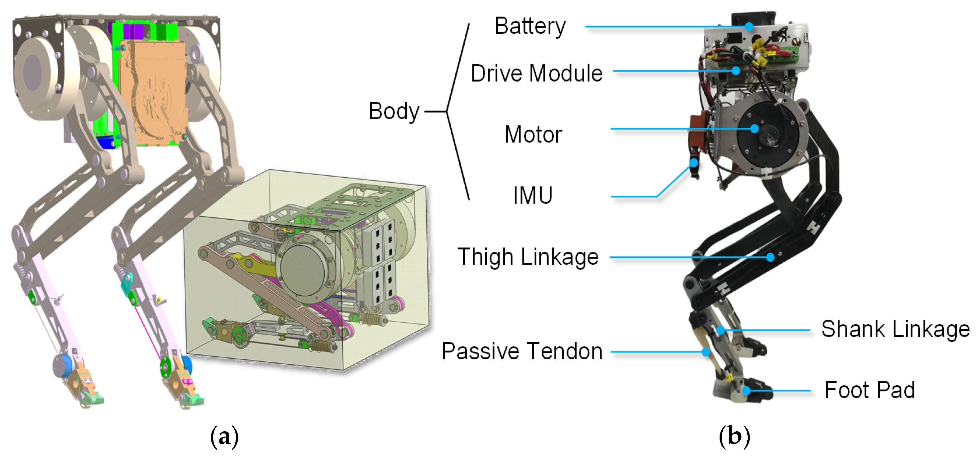
2.1. General Description of the Bipedal Robot Prototype

The basic components of the self-developed bipedal robot are shown in Figure 1. In general, the robot has 4 active DoFs, with co-axial actuations at the hip for each leg. The configuration of the leg is evolved based on a five-bar mechanism that exhibits deployable features with sufficient load capacity, offering a compact storage size, as shown in Figure 1a, for portable convenience. High-quality carbon fiber is used to fabricate a single leg, with lightweight and high-strength properties. The co-axial actuation mainly comprises a two-drive module, which is a combination of a DC brushless motor (rated speed of 2200 rpm, peak torque of 2.08 Nm), single-stage planetary reducer (gear ratio of 9), contactless 12-bit absolute encoder, and servo driver (ELMO G-WLTWIR50/100). The upper body in the aluminum frame carries the IMU (XSENS, MTi-G-710) and the battery unit. The total weight of this self-contained bipedal robot is approximately 4.08 kg, with a natural standing height of 0.45 m. The basic specifications of the robot are given in

Table 1. Basic specifications of the bipedal robot.

Specifications	Value	Unit
Total mass	4.08	kg
Body mass	3.36	kg
Leg mass (single)	0.34	kg
Foot mass (single)	0.04	kg
Natural standing height	0.45	m
Body height	0.25	m
Body width	0.38	m
Foot pad length	0.04	m
Storage size (leg folded)	0.35 × 0.27 × 0.19	m3

.

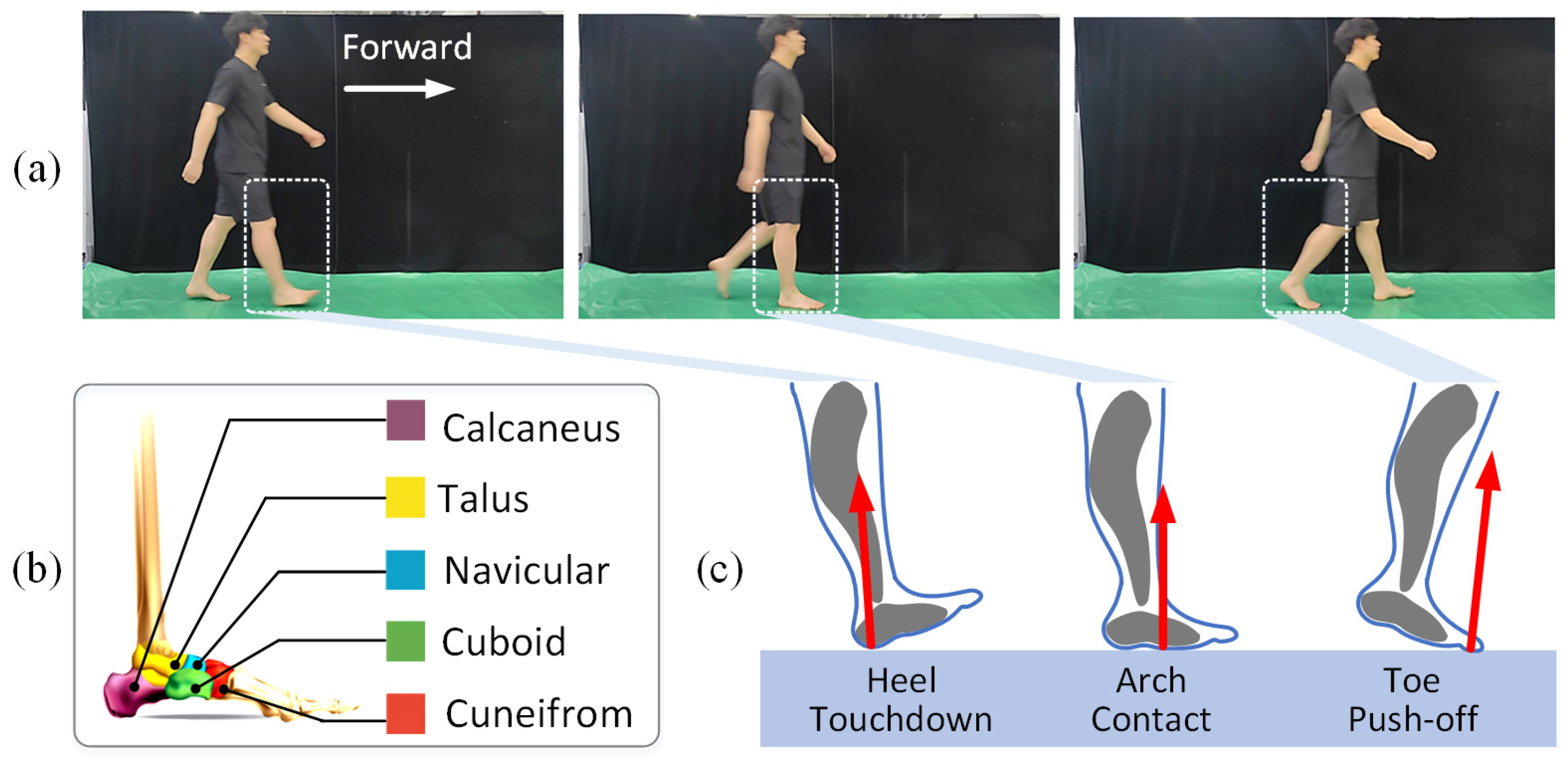
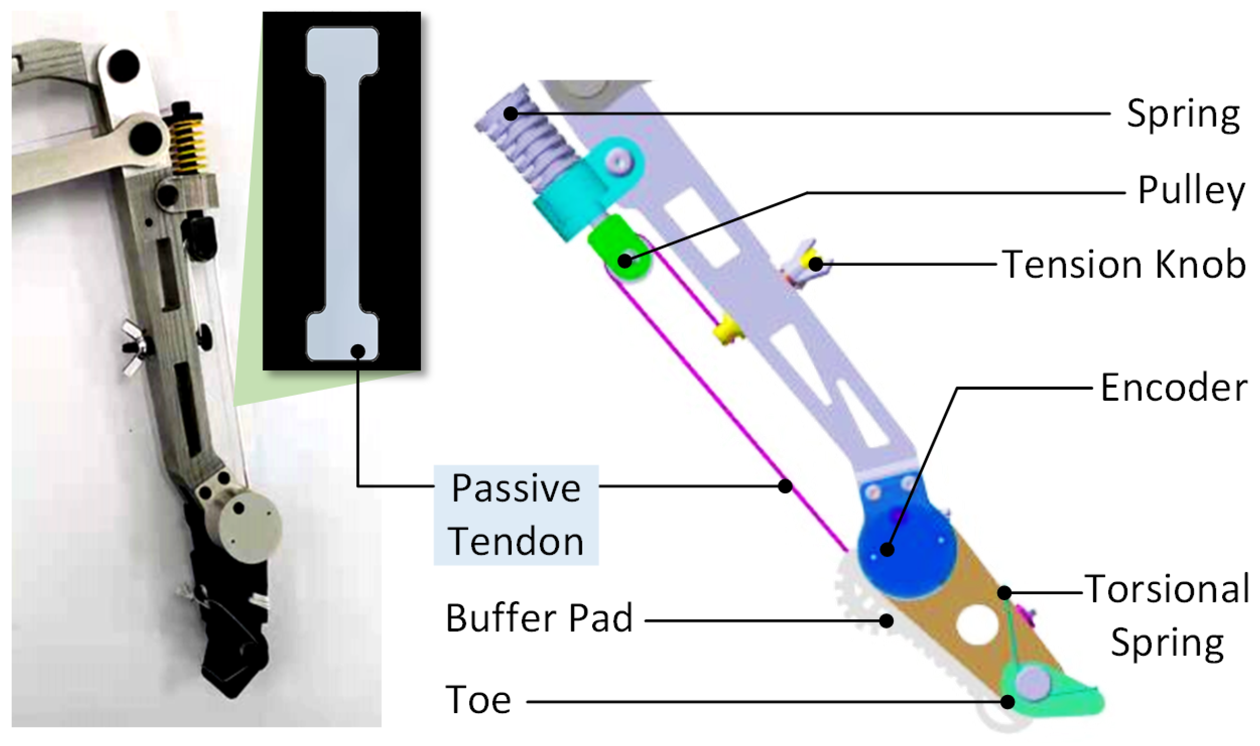
2.2. Inspiration and Design of Passive Tendon

The main design concept of the passive tendon is inspired by the muscle-tendon complex [24] around the ankle joint of humans, as shown in Figure 2b. According to the recent findings in anatomy [25] and biomechanics [26], the interaction between the series elastic elements and the contractile elements from the muscle-tendon unit exhibiting compliant behavior plays a positive role in absorbing and releasing mechanical energy during walking. Particularly, the ankle plantar flexors together with the soleus and gastrocnemius can improve the energy efficiency by appropriately using the elastic strain energy of the tendon in pace with the human gait cycle. As shown in Figure 2a, we conduct the walking test with a forceplate (KISTLER, 9260AA6) to concurrently measure the ground reaction force. One experienced subject (male, age 25 years, body mass 74.5 kg, height 183 cm, leg length 105 cm) participated in the trials on a flat surface. Different contact stages in the stance phase of the stride cycle, including the heel touchdown, arch contact, and toe push-off [27], are illustrated in Figure 2c.

The design guideline of the passive tendon in the bipedal robot can be summarized as the following aspects. An elastic element (such as passive tendon) with favorable compliance is expected to connect the shank and the foot pad, acting as the ankle plantar flexors. The timing of the tendon extension and contraction should be well tuned in accordance with different contact stages of the foot in the stance phase during walking. To this end, we propose a novel passive tendon-based scheme that mimics the function of the ankle plantar flexor, as shown in Figure 3. The material of the artificial tendon is selected as the emulsion (XY-8625HB, thickness 2 mm, total mass 14.2 g) and fabricated by laser cutting after cold molding. Inspired by the antagonistic movement of the triceps surae around the calcaneus during human walking, the tendon is attached inside the groove of the footpad, and the other end is fixed at the tension knob on the shank bypass of the spring-loaded tension pulley. The torsional spring is applied at the connection between the toe and the foot pad, providing a restoring torque for the toe with respect to the arch structure of the foot pad. This mechanism is enabled at the toe push-off stage of the stance phase to allow rapid cessation of contact (especially in fast walking scenario). Last but not least, a fluorelastomer buffer layer (Dyneon FE) is integrated along the foot pad to mitigate the impulsive effect when the foot touches ground at the stance phase of each gait cycle.

2.3. Sensors and Electical Layout

To facilitate the state estimation and locomotion control of the bipedal robot, diverse sensors are equipped on the prototype, offering a comprehensive sensory feedback. The body posture is measured by the IMU attached on the upper body as aforementioned in Section 2.1. The leg configuration and position/orientation information can be determined by solving the forward kinematics of the five-bar mechanism according to the dual encoders (RLS Inc., Ljubljana, Slovenia, RMB20SC) from the co-axial drive modules. An affordable encoder that measures the rotation angle of the ankle joint for each leg to indirectly detect the contact stage is mounted coaxially to the ankle joint instead of applying a fragile load cell in frequent foot–ground impact. Other necessary information (i.e., hardware temperature, battery capacity) are simultaneously sampled by the DAQ unit.

The structure of the electrical system is shown in Figure 4. The real-time control platform of the robot is a compact-size mini personal computer (Intel Inc., Santa Clara, CA, USA, NUC-8iB5EHS, 2.3 GHz), which executes tasks that include walking gait generation, joint-level motion planning, whole-body control, data acquisition of sensory feedback, and high-level command interpretation from the user. The four motors’ commands are sent to the ELMO servo driver boards via the EtherCAT bus at 1 kHz. The corresponding feedback data, including the motor currents and joint angles, are transmitted to the computer in turn. The body posture measured by the IMUis sampled by the self-developed PCB board via the SSI protocol and transmitted as the uplink data to the computer via the USB port at rate of 0.5 kHz. The contact stage of each foot is identified by the ankle encoder with the sampling rate of 1 kHz. Since the encoder-based contact detection is crucial for the walking control of the bipedal robot, the original signal of the encoder at the ankle joint is filtered, and a threshold value is also utilized to identify the foot–ground contact. In the high-level regulation, the user GUI interface is established on the host PC so as to monitor the key state of the robot and rebuild the walking scenario in a concurrent simulation environment according to the sensory feedback data. The basic motion order to regulate the specific actions of the robot is artificially maneuvered by an operator handle communicated via wireless Bluetooth at 2.4 GHz to the control platform.

3. Dynamic Modeling and Gait Synthesis of the Bipedal Robot

This section mainly addresses the modeling and walking gait analysis of the bipedal robot. The closed-chain constraints of the robot with coaxial actuations of the leg with the five-bar mechanism is discussed. Subsequently, the unified dynamic model of the bipedal robot is presented. The walking gait is investigated to prepare for controller design in Section 4.

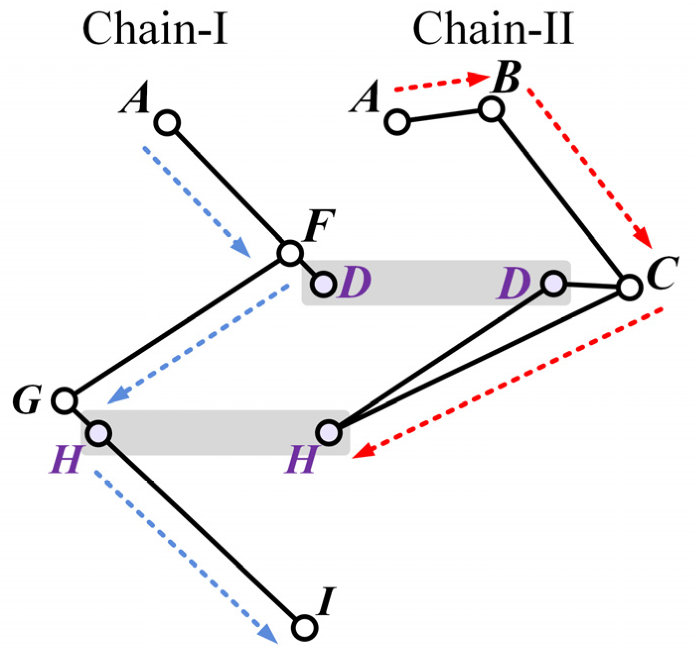
3.1. Kinematics of the Leg with Coaxial Actuations

The coordinates of the single-leg together with the identified hinge points of the five-bar mechanism on the sagittal plane are shown in Figure 5. Without loss of generality, we take the right-side leg as an example. Taking the intersection point O_b of the axis of the coaxial drive motors and the sagittal plane as the origin of the body coordinate Σ-XO_bY, the angular displacements of the coaxial actuations can be defined by measuring the driven links AB and AD in counterclockwise direction with respect to the positive X-axis, obtaining the dual-input variable θ_AB and θ_AD. In the quadrangle ABCD, the coordinate (x_C, y_C) of the pivot C can be determined based on the geometry parameters of link BC and CD and the coordinates (x_B, y_B) and (x_D, y_D) of the pivot B and D, respectively. To facilitate the kinematical calculation, the quadrangle DFGH is enforced into a parallelogram such that the condition l_AD = l_HI holds. By combining the geometric relationship between ΔCDH and hinge points G, H, and I, the foot coordinates (x_I, y_I) can be directly acquired. We omit the tedious geometry-related derivations for brevity. The velocity mapping from the coaxial actuation to the foot end point I can be written as

$$\left[\begin{array}{l}{\dot{x}}_{\mathrm{I}}\\ {\dot{y}}_{\mathrm{I}}\end{array}\right]={\mathit{M}}_a\left[\begin{array}{l}{\dot{\theta }}_{\mathrm{AD}}\\ {\dot{\theta }}_{\mathrm{DH}}\end{array}\right],$$

(1)

where x_I and y_I are the horizontal and vertical position of the foot end point I, respectively. M_a is the corresponding mapping matrix and satisfies

$${\mathit{M}}_a=\left[\begin{array}{ll}-2l_{\mathrm{AD}}\sin {\theta }_{\mathrm{AD}},& -l_{\mathrm{DH}}\sin {\theta }_{\mathrm{DH}}\\ 2l_{\mathrm{AD}}\cos {\theta }_{\mathrm{AD}},& l_{\mathrm{DH}}\cos {\theta }_{\mathrm{DH}}\end{array}\right].$$

(2)

According to the local view of Figure 5, θ_DH = θ_CD + π − θ_CDH holds. Since θ_CDH remains constant in ΔCDH, we have the following relation:

$${\dot{\theta }}_{\mathrm{DH}}={\dot{\theta }}_{\mathrm{CD}}.$$

(3)

In the closed-chain ABCD, the actuated angles θ_AB and θ_AD and the associated angles θ_BC and θ_CD satisfy the following relation:

$$\left\{\begin{array}{c}{l}_{\mathrm{AB}}\cos {\theta }_{\mathrm{AB}}+l_{\mathrm{BC}}\cos {\theta }_{\mathrm{BC}}=l_{\mathrm{AD}}\cos {\theta }_{\mathrm{AD}}+l_{\mathrm{CD}}\cos {\theta }_{\mathrm{CD}}\\ l_{\mathrm{AB}}\sin {\theta }_{\mathrm{AB}}-l_{\mathrm{BC}}\sin {\theta }_{\mathrm{BC}}=l_{\mathrm{AD}}\sin {\theta }_{\mathrm{AD}}-l_{\mathrm{CD}}\sin {\theta }_{\mathrm{CD}}\end{array}\right..$$

(4)

By acquiring the first-order derivative of Equation (4) on both sides, the angular velocity mapping can be obtained via

$${\mathit{M}}_{\mathrm{b}}\left[\begin{array}{l}{\dot{\theta }}_{\mathrm{AB}}\\ {\dot{\theta }}_{\mathrm{AD}}\end{array}\right]={\mathit{M}}_c\left[\begin{array}{l}{\dot{\theta }}_{\mathrm{BC}}\\ {\dot{\theta }}_{\mathrm{CD}}\end{array}\right],$$

(5)

where the mapping matrices M_b and M_c are conveyed as

$${\mathit{M}}_{\mathrm{b}}=\left[\begin{array}{ll}{l}_{\mathrm{AB}}\sin {\theta }_{\mathrm{AB}},& -l_{\mathrm{AD}}\sin {\theta }_{\mathrm{AD}}\\ l_{\mathrm{AD}}\cos {\theta }_{\mathrm{AD}},& -l_{\mathrm{AD}}\cos {\theta }_{\mathrm{AD}}\end{array}\right],{\mathit{M}}_c=\left[\begin{array}{ll}-l_{\mathrm{BC}}\sin {\theta }_{\mathrm{BC}},& l_{\mathrm{CD}}\sin {\theta }_{\mathrm{CD}}\\ l_{\mathrm{BC}}\cos {\theta }_{\mathrm{BC}},& -l_{\mathrm{CD}}\cos {\theta }_{\mathrm{CD}}\end{array}\right].$$

(6)

Let ${\mathit{M}}_d={\mathit{M}}_c^{-1}{\mathit{M}}_{\mathrm{b}}$, then ${\dot{\theta }}_{\mathrm{CD}}$ can be solved in Equation (5) as

$${\dot{\theta }}_{\mathrm{CD}}={\mathit{M}}_d(2,2){\dot{\theta }}_{\mathrm{AD}}+{\mathit{M}}_d(2,1){\dot{\theta }}_{\mathrm{AB}},$$

(7)

where M_d(i, j) represents the element at the i-th row and the j-th column of the original matrix M_d. Eventually, the velocity mapping between the foot and the coaxial actuations can be constructed as

$$\left[\begin{array}{l}{\dot{x}}_{\mathrm{I}}\\ {\dot{y}}_{\mathrm{I}}\end{array}\right]={\mathit{J}}_{foot}\left[\begin{array}{l}{\dot{\theta }}_{\mathrm{AD}}\\ {\dot{\theta }}_{\mathrm{AB}}\end{array}\right],$$

(8)

where J_foot is the Jacobian from the toe to the actuated joints and satisfies

$${\mathit{J}}_{\mathrm{foot}}={\mathit{M}}_a\left[\begin{array}{cc}1& 0\\ {\mathit{M}}_d(2,2)& {\mathit{M}}_d(2,1)\end{array}\right].$$

(9)

3.2. Dynamic Model of the Bipedal Robot

The single leg of the bipedal robot is topologically a five-bar mechanism containing a closed-chain ABCDF. The generalized coordinate of the bipedal robot q is selected as $\mathit{q}={[{\mathit{q}}_{body}^T,{\mathit{q}}_{active}^T,{\mathit{q}}_{passive}^T]}^T\in {ℝ}^{15\times 1}$, and the vector of body q_body collects the position and posture of the upper body of the robot with q_body = (x_b, y_b, θ_b)^T, the vector of actuation collects the angular positions of all the active linkages for the left and right side of legs with q_active = (θ_ABL, θ_ADL, θ_ABR, θ_ADR)^T, and the vector of under-actuations collects the angular positions of all the passive linkages for the left and right side of legs with q_passive= (q_BCL, q_CDL, q_FGL, q_GIL, q_BCR, q_CDR, q_FGR, q_GIR)^T. Therefore, the dynamic model of the bipedal robot with the five-bar mechanism can be uniformly conveyed as

$$\mathit{M}\left(\mathit{q}\right)\ddot{\mathit{q}}+\mathit{C}\left(\mathit{q},\dot{\mathit{q}}\right)=\mathit{S}\mathit{\tau }+{\displaystyle \sum _{i\in \{R, L\}}{\chi }_i{\mathit{J}}_i^T{\mathit{\lambda }}_i},$$

(10)

where M is the generalized inertia matrix that depends only on q, C is the generalized bias force that depends on both q and $\dot{\mathit{q}}$, S is the selection matrix of actuation associated with q_active, τ is the torque vector of the four active linkages for both legs with τ = (τ_ABL, τ_ADL, τ_ABR, τ_ADR)^T, λ_i= (λ_ix, λ_iy)^T is the ground reaction force of the i-th contact foot with the corresponding Jacobian J_i, and χ_i is the detection coefficient of the i-th contact foot with the assignment rule shown in

Table 2. Assignment rule of the detection coefficient during different foot contact phases.

Foot Contact State	Left-Side χL	Right-Side χR	Gait Phase
Double support	1	1	Stance
Double take-off	0	0	Flight
Left-side leg in stance	1	0	Stance
Right-side leg in stance	0	1	Stance

. The subscript “L” and “R” denote the left and right side of each leg. Note the value of χ_R + χ_L denotes the number of feet in contact with the ground.

For the leg touches ground, the stationary foot is assumed throughout this paper to have no slippage occurring in the stance phase. Hence, the contact constraint becomes

$${\mathit{J}}_c\ddot{\mathit{q}}+{\dot{\mathit{J}}}_c\dot{\mathit{q}}=\mathbf{0},$$

(11)

where ${\mathit{J}}_c\in {ℝ}^{2\left({\chi }_R+{\chi }_L\right)\times 15}$ is the contact Jacobian. Then, a feasible foothold can be further defined as the condition that all the contact forces from the feet in stance satisfy the friction limits. In other words, the ground reaction force λ_i of the i-th contact foot should be restricted inside the cone of friction with

$$\left|{\lambda }_{ix}\right|\le \mu {\lambda }_{iy} \mathrm{and} {\lambda }_{iy}>0.$$

(12)

For the five-bar mechanism of a single leg, the closed-chain constraints should be addressed so that the node movement of individual open-chain links can be matched [28]. We hereby take the left-side leg as an example and then extend to both sides to construct the closed-chain constraint of q. As illustrated in Figure 6, the five-bar mechanism with kinematical closed chains can be topologically divided into two open chains, namely AFD→FG→GHI and AB→BC→CDH. We select the public nodes D and H for constructing the closed-chain constraints due to the existence of closed-loop ABCDF and FDHG. The velocities of the nodes D and H should be self-consistent between both open chains; thus, we have

$$\left\{\begin{array}{l}{\mathit{J}}_{ch1-L}^D\dot{\mathit{q}}={\mathit{J}}_{ch2-L}^D\dot{\mathit{q}}\\ {\mathit{J}}_{ch1-L}^H\dot{\mathit{q}}={\mathit{J}}_{ch2-L}^H\dot{\mathit{q}}\end{array}\right.,$$

(13)

where ${\mathit{J}}_{ch\left(••\right)-L}^{\left(•\right)}$ denotes the velocity Jacobian from the generalized coordinate q to the public node (●) by using the chain (●●) for the left-side leg. Similarly, we can also obtain the acceleration consistence constraint for the nodes D and H by differentiating the both sides of Equation (13) with respect to time as

$$\left\{\begin{array}{l}{\mathit{J}}_{ch1-L}^D\ddot{\mathit{q}}+{\dot{\mathit{J}}}_{ch1-L}^D\dot{\mathit{q}}={\mathit{J}}_{ch2-L}^D\ddot{\mathit{q}}+{\dot{\mathit{J}}}_{ch2-L}^D\dot{\mathit{q}}\\ {\mathit{J}}_{ch1-L}^H\ddot{\mathit{q}}+{\dot{\mathit{J}}}_{ch1-L}^H\dot{\mathit{q}}={\mathit{J}}_{ch2-L}^H\ddot{\mathit{q}}+{\dot{\mathit{J}}}_{ch2-L}^H\dot{\mathit{q}}\end{array}\right.,$$

(14)

Note that the identical formulation holds for the right-side leg; therefore, we can extend the acceleration constraints in Equation (14) to both legs, yielding the unified vector version of the closed-chain constraints of q as

$${\mathit{J}}_{CC}\ddot{\mathit{q}}+{\dot{\mathit{J}}}_{CC}\dot{\mathit{q}}=0,$$

(15)

where J_CC is the combined Jacobian of the closed-chain constraints for both legs.

$${\mathit{J}}_{CC}=\left(\begin{array}{l}{\mathit{J}}_{ch1-L}^D-{\mathit{J}}_{ch2-L}^D\\ {\mathit{J}}_{ch1-L}^H-{\mathit{J}}_{ch2-L}^H\\ {\mathit{J}}_{ch1-R}^D-{\mathit{J}}_{ch2-R}^D\\ {\mathit{J}}_{ch1-R}^H-{\mathit{J}}_{ch2-R}^H\end{array}\right).$$

(16)

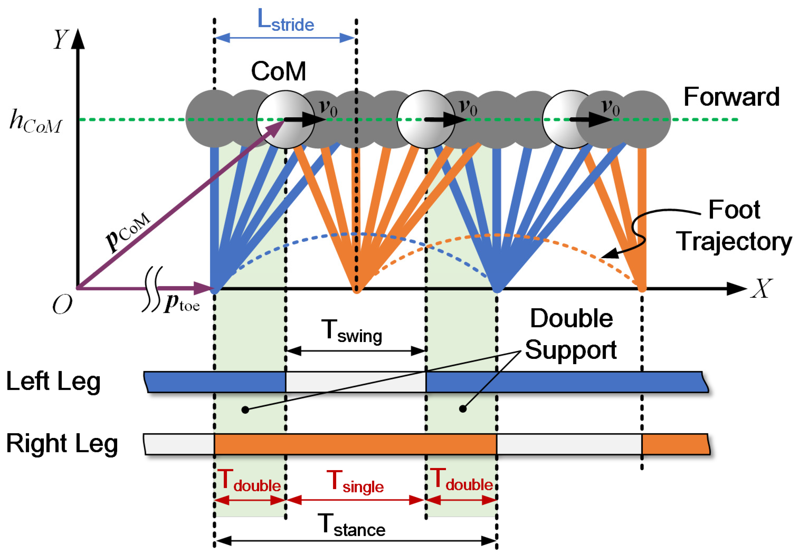
3.3. LIP Model-Based Walking Gait Synthesis

The Linear Inverted Pendulum (LIP) model with physically feasible modifications is widely regarded as a fundamental benchmark for both gait generation [29] and dynamic locomotion control [30] for bipedal robots. In this paper, we employ the LIP model as the basic template to generate the prescribed CoM trajectory of the bipedal robot. The adopted LIP model together with the walking gait division is shown in Figure 7. The walking gait cycle T_walk is determined by the swing duration T_swing and the stance duration T_stance, with T_walk = T_swing + T_stance. Particularly, the stance duration can be further divided into the single support duration T_single and the double support duration T_double. The former T_single directly equals T_swing. The latter T_double can be easily calculated by using T_double = (T_stance − T_swing)/2, as illustrated in Figure 7. According to the basic assumption of the original LIP model [31], the LIP model is conventionally composed of a point mass at the CoM and a massless extendable leg that alternately touches the ground. We mark the touch-down event (when the leg contacts the ground) and the lift-off event (when the leg leaves the ground) as TD and LO, respectively. In the single support duration, the ground reaction force F_GRF of the LIP model can be calculated as

$${\mathit{F}}_{\mathrm{GRF}}=\left({\mathit{p}}_{\mathrm{CoM}}-{\mathit{p}}_{\mathrm{foot}}\right)\frac{mg}{h_{\mathrm{CoM}}},$$

(17)

where p_CoM = [x_CoM, y_CoM]^T is the position vector of the CoM of the LIP model in the world coordinate system. p_toe = [x_toe, y_toe]^T is the position vector of the foot at the stance phase in the current gait cycle. h_CoM is the ideal CoM height of the LIP model. The CoM dynamics at the single-leg duration can be further depicted as

$$\left[\begin{array}{l}{\ddot{x}}_{\mathrm{CoM}}\\ {\ddot{y}}_{\mathrm{CoM}}\end{array}\right]=\frac{g}{h_{\mathrm{CoM}}}\left[\begin{array}{l}{x}_{\mathrm{CoM}}-x_{\mathrm{toe}}\\ y_{\mathrm{CoM}}-h_{\mathrm{CoM}}\end{array}\right].$$

(18)

Note that h_CoM remains constant from stride to stride. Equation (18) can be reduced to

$${\ddot{x}}_{\mathrm{CoM}}-{\omega }^2{x}_{\mathrm{CoM}}=-{\omega }^2{x}_{toe},$$

(19)

where $\omega =\sqrt{g/h_{\mathrm{CoM}}}$ is the eigenvalue of Equation (19). Given the initial velocity v₀ and horizontal position x₀ of the CoM, the movement toward the forward direction can be determined by

$$\left\{\begin{array}{l}{x}_{\mathrm{CoM}}(t)=a{e}^{\omega t}+b{e}^{-\omega t}+x_{\mathrm{toe}}\\ {\dot{x}}_{\mathrm{CoM}}(t)=\omega a{e}^{\omega t}-\omega b{e}^{-\omega t}\end{array}\right.,$$

(20)

where the coefficients a and b are given by a = (x₀ + v₀/ω)/2 and b = (x₀-v₀/ω)/2, respectively. For the double support duration, the CoM dynamics can be written as

$${\ddot{x}}_{\mathrm{CoM}}=0,$$

(21)

which implies that the CoM moves at a constant speed ${\dot{x}}_{\mathrm{CoM}}$ in the double support duration. Taking the right leg in Figure 7 as an example, the stance phase of the right leg is composed by two double support durations T_double and one single support duration T_single. According to Equation (21), the distance the CoM travels in each double support duration is determined by

$$v_0{T}_{\mathrm{double}}=\frac{L_{\mathrm{stride}}}{2},$$

(22)

where L_stride is the distance between two contact toes. In the single support duration T_single, the movement of the CoM at the initial time-instant satisfies the following boundary conditions:

$$\left\{\begin{array}{l}{x}_{\mathrm{CoM}}(T_{\mathrm{single}}^{\mathrm{in}})=x_{\mathrm{toe}}+\frac{L_{\mathrm{stride}}}{2}\\ {\dot{x}}_{\mathrm{CoM}}(T_{\mathrm{single}}^{\mathrm{in}})=v_0\end{array}\right.,$$

(23)

where $T_{\mathrm{single}}^{\mathrm{in}}$ is the initial time-instant of the single support duration. Note that the distance the CoM travels in this period is L_stride. We have the following boundary conditions at the ending time-instant:

$$\left\{\begin{array}{l}{x}_{\mathrm{CoM}}(T_{\mathrm{single}}^{\mathrm{out}})=x_{\mathrm{toe}}+\frac{3L_{\mathrm{stride}}}{2}\\ {\dot{x}}_{\mathrm{CoM}}(T_{\mathrm{single}}^{\mathrm{out}})=v_0\end{array}\right.,$$

(24)

where $T_{\mathrm{single}}^{\mathrm{out}}$ is the initial time-instant of the single support duration.

Let $\mathit{S}\left(t\right)={\left[x_{CoM}\left(t\right),{\dot{x}}_{CoM}\left(t\right)\right]}^T$ be the state vector of the CoM. The motion planning task of the LIP model on the sagittal plane can be formulated by solving the shooting problem.

$$\begin{array}{cc}\hfill \underset{u={[L_{\mathrm{stride}},T_{\mathrm{single}}]}^T}{\mathrm{minimize}}& {\left[\mathit{S}\left(T_{\mathrm{single}}+2T_{\mathrm{double}}\right)-{\mathit{S}}^{des}\right]}^T\mathit{Q}\left[\mathit{S}\left(T_{\mathrm{single}}+2T_{\mathrm{double}}\right)-{\mathit{S}}^{des}\right]\hfill \\ \hfill \mathrm{subject} \mathrm{to} {\ddot{x}}_{\mathrm{CoM}}=& {\omega }^2\left(x_{\mathrm{CoM}}-x_{\mathrm{toe}}\right)\hfill \\ \hfill x_{\mathrm{CoM}}(0)=& x_{\mathrm{toe}}+L_{stride}/2 \hfill \\ \hfill {\dot{x}}_{\mathrm{CoM}}(0)=& v_0\hfill \\ \hfill T_{\mathrm{double}}=& L_{stride}/\left(2v_0\right)\hfill \\ \hfill \Delta x_{\min }\le & x_{\mathrm{CoM}}-x_{toe}\le \Delta x_{\max }\hfill \\ \hfill T_{\min }\le & T_{\mathrm{single}}+2T_{\mathrm{double}}\le T_{\max }\hfill \end{array}$$

(25)

where Q = diag(w₁, w₂) is a weight matrix. Δx_min and Δx_max are the admissible lower and upper bound of the displacement of the CoM, respectively. T_min and T_max are the lower and upper bound of the stance duration of the LIP model. ${\mathit{S}}^{des}={\left[x_{\mathrm{CoM}}^{\mathrm{des}},{\dot{x}}_{\mathrm{CoM}}^{\mathrm{des}}\right]}^T$ is the desired state vector of S. u is the tunable parameter collection with u = [L_stride T_single]^T. For consecutive walking strides, the motion planning algorithm of the LIP model is summarized as shown in Algorithm 1.

Algorithm 1: Motion Planning of the LIP Model on the Sagittal Plane

Input: Desired CoM state at the ending of single support duration Sdes    Desired walking speed at double support duration v0    Height of the CoM hCoM    Position of the CoM $x_{\mathrm{CoM},k}^{\mathrm{in}}$    Start time of the stance phase $T_{\mathrm{stance},k}^{\mathrm{in}}$

Output: Trajectory of the CoM xCoM

1: $\omega \leftarrow \sqrt{g/h_{\mathrm{CoM}}}$ 2: ${\mathit{u}}_k\leftarrow \underset{L_{\mathrm{stride}},T_{\mathrm{single}}}{\arg \min } {‖\mathit{S}\left(T_{\mathrm{single}}+2L_{stride}/\left(2v_0\right)\right)-{\mathit{S}}^{des}‖}_{\mathit{Q}}$ by solving shooting problem (25) 3: $L_{\mathrm{stride},k}\leftarrow {\mathit{u}}_k(1)$ 4: $T_{\mathrm{single},k}\leftarrow {\mathit{u}}_k(2)$ 5: $T_{\mathrm{double},k}\leftarrow L_{\mathrm{stride},k}/\left(2v_0\right)$ 6: Compute trajectory xCoM using Equation (21) for the double support duration $\left[T_{\mathrm{stance},k}^{\mathrm{in}},T_{\mathrm{stance},k}^{\mathrm{in}}+T_{\mathrm{double},k}\right]$ 7: Compute trajectory xCoM using Equation (20) for the single support duration $\left[T_{\mathrm{stance},k}^{\mathrm{in}}+T_{\mathrm{double},k},T_{\mathrm{stance},k}^{\mathrm{in}}+T_{\mathrm{double},k}+T_{\mathrm{single},k}\right]$ 8: Compute trajectory xCoM using Equation (21) for the double support duration $\left[T_{\mathrm{stance},k}^{\mathrm{in}}+T_{\mathrm{double},k}+T_{\mathrm{single},k},T_{\mathrm{stance},k}^{\mathrm{in}}+2T_{\mathrm{double},k}+T_{\mathrm{single},k}\right]$

4. Control Framework of the Bipedal Robot

This section details the control framework of the bipedal robot by using the LIP model to generate the CoM’s trajectory. In the swing leg control, the Beizer polynomial-based trajectory is created for the leg in the swing phase. Subsequently, the whole body control (WBC) is established to reproduce the LIP model’s behavior as the target dynamics. A double-layer framework for the bipedal robot is further developed to achieve stable walking for the bipedal robot.

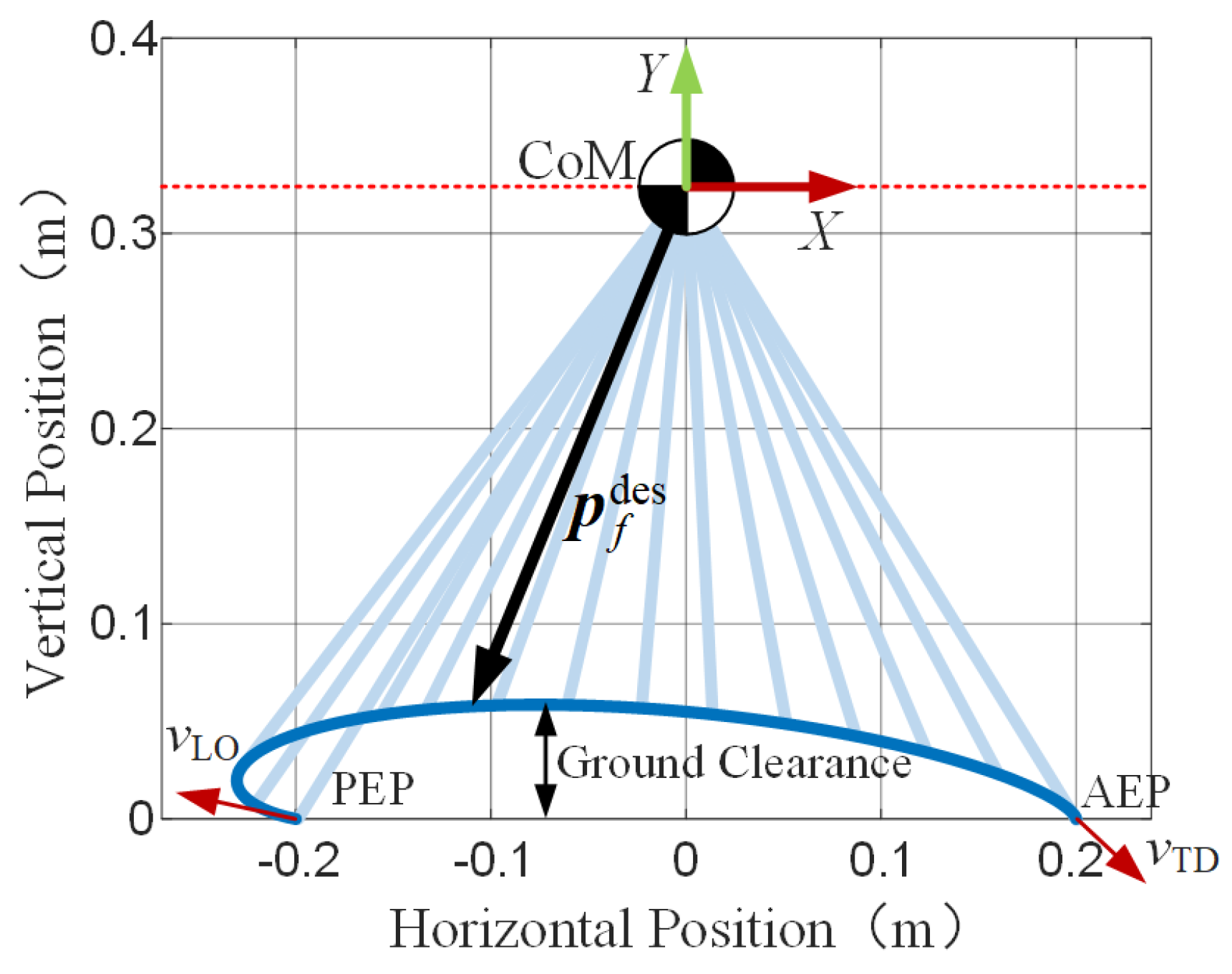
4.1. Swing Leg Control

The trajectory of the swing leg on the sagittal plane is shown in Figure 8. The planar curve is generated based on the Bezier polynomial to describe a specific swing pattern of the foot end in the centroid coordinate system. The basic requirements of the swing leg trajectory lie in the following aspects. First, the anterior extreme position (AEP) and the posterior extreme position (PEP) of the foot should be restrained with the reachable space of the single leg. Second, the swing apex should be well tuned to provide sufficient ground clearance, resulting in a safe sweep motion without stumble. Last, the stride length should be appropriate, matching the rhythmical feature of the LIP model. In this paper, we select the desired foot position ${\mathit{p}}_f^{des}$ in the swing phase as

$${\mathit{p}}_f^{des}=\left(\begin{array}{l}{\mathit{p}}_f^{des}\left(x\right)\\ {\mathit{p}}_f^{des}\left(y\right)\end{array}\right)={\displaystyle \sum _{j=0}^B\left(\begin{array}{l}B\\ j\end{array}\right)}{\mathit{p}}_j{(1-t)}^{B-j}{t}^j,$$

(26)

where p_j = (p_j(x), p_j(y))^T is the control point of the Bezier curve, and B is the order of the Bezier polynomials. As shown in Figure 8, the scheduled stride length of each swing is 0.4 m with respect to the CoM. The ground clearance approaches 0.059 m.

The task of the swing leg control is to track the foot trajectory planned in Equation (26). For the actuation angles q_active = (θ_ABL, θ_ADL, θ_ABR, θ_ADR)^T of both legs, the PD-type command for each angle in q_active is given by

$${\ddot{q}}_i^{cmd}={\ddot{q}}_i^{des}+K_{D,i}\left({\dot{q}}_i^{des}-{\dot{q}}_i\right)+K_{P,i}\left(q_i^{des}-q_i\right),$$

(27)

where $q_i\in \{{\theta }_{ABL},{\theta }_{ADL},{\theta }_{ABR},{\theta }_{ADR}\}$ denotes the arbitrary active angle from q_active, $q_i^{des}$ denotes the desired value of q_i and can be directly obtained by solving the inverse-kinematics of the single-leg, ${\dot{q}}_i^{des}$ and ${\ddot{q}}_i^{des}$ are the corresponding desired angular velocity and acceleration of q_i, respectively, and K_D,I and K_P,I denote the coefficients of the PD controller for q_i.

4.2. Stance Leg Control

As the leg contacts the ground, the main task of the controller is to enforce the bipedal robot to produce the dynamic behavior of the LIP model. In other words, the trajectory of the CoM of the robot will be generated by the LIP model. Referring to the full-order system of the bipedal robot, we select $\ddot{\mathit{q}}$ and τ as optimization parameters. The former parameter collects the specific movements of legs, while the latter collects the actuation inputs of four motors. The inverse dynamics-based WBC optimization can be further constructed by creating a quadratic programming (QP) problem, as follows:

$$\begin{gathered} \begin{array}{l}\underset{\ddot{\mathit{q}},\tau }{\mathrm{minimize}} {\left({\ddot{\mathit{x}}}_{CoM}^{cmd}-{\ddot{\mathit{x}}}_{CoM}\right)}^T{\mathit{W}}_{CoM}\left({\ddot{\mathit{x}}}_{CoM}^{cmd}-{\ddot{\mathit{x}}}_{CoM}\right)\end{array} \\ \begin{array}{cc}\hfill \mathrm{subject} \mathrm{to} \mathit{M}\left(\mathit{q}\right)\ddot{\mathit{q}}+\mathit{C}\left(\mathit{q},\dot{\mathit{q}}\right)& =\mathit{S}\mathit{\tau }+{\displaystyle \sum _{i\in \{R, L\}}{\chi }_i{\mathit{J}}_i^T{\mathit{\lambda }}_i}\hfill \\ \hfill {\mathit{J}}_{CoM}\ddot{\mathit{q}}+{\dot{\mathit{J}}}_{CoM}\dot{\mathit{q}}& ={\ddot{\mathit{x}}}_{CoM}\hfill \\ \hfill {\mathit{J}}_c\ddot{\mathit{q}}+{\dot{\mathit{J}}}_c\dot{\mathit{q}}& =\mathit{0}\hfill \\ \hfill {\mathit{J}}_{CC}\ddot{\mathit{q}}+{\dot{\mathit{J}}}_{CC}\dot{\mathit{q}}& =\mathit{0}\hfill \\ \hfill {\mathit{q}}_{\min }\le \mathit{q}& \le {\mathit{q}}_{\max }\hfill \\ \hfill {\mathit{\tau }}_{\min }\le \mathit{\tau }& \le {\mathit{\tau }}_{\max }\hfill \\ \hfill \left|{\lambda }_{ix}\right|\le & \mu {\lambda }_{iy} \mathrm{and} {\lambda }_{iy}>0\hfill \end{array}, \end{gathered}$$

(28)

where x_CoM is the CoM position of the bipedal robot, J_CoM is the corresponding mapping Jacobian between $\dot{\mathit{q}}$ and ${\dot{\mathit{x}}}_{CoM}$, W_CoM is the diagonal weighted matrix, and ${\ddot{\mathit{x}}}_{\mathrm{CoM}}^{cmd}$ represents the task dynamics referring to the LIP model and has the following second-order formulation:

$${\ddot{\mathit{x}}}_{CoM}^{cmd}={\ddot{\mathit{x}}}_{CoM}^{des}+{\mathit{K}}_{D,CoM}\left({\dot{\mathit{x}}}_{CoM}^{des}-{\dot{\mathit{x}}}_{CoM}\right)+{\mathit{K}}_{P,CoM}\left({\mathit{x}}_{CoM}^{des}-{\mathit{x}}_{CoM}\right),$$

(29)

where ${\ddot{\mathit{x}}}_{CoM}^{des}$ represents the target dynamics generated by the LIP model acquired by using Algorithm 1. K_D,CoM and K_P,CoM are both positive definite gain matrices. Note that if the error of the target dynamics is defined as ${\mathit{e}}_{CoM}={\mathit{x}}_{CoM}^{des}-x_{CoM}$, then plugging e_CoM into Equation (29) will yield the error dynamics:

$${\ddot{\mathit{e}}}_{CoM}+{\mathit{K}}_{D,CoM}{\dot{\mathit{e}}}_{CoM}+{\mathit{K}}_{P,CoM}{\mathit{e}}_{CoM}=\mathit{0}.$$

(30)

By carefully selecting the elements of K_D,CoM and K_P,CoM, the ordinary differential Equation (30) is Hurwitz stable, which implies that the target dynamics ${\ddot{\mathit{x}}}_{CoM}={\mathit{J}}_{CoM}\ddot{\mathit{q}}+{\dot{\mathit{J}}}_{CoM}\dot{\mathit{q}}$ is consistently unique without interference [32]. As to the constraints listed in Equation (28), the aforementioned seven constraints concentrate on the whole-body dynamics of the robot, the task dynamics of the CoM associated with the LIP model, the foot contact of the leg at stance, the closed-chain constraints of the five-bar mechanism, the reachable workspace of individual joints, the physical limitations of the actuators, and the friction restriction for the ground reaction forces.

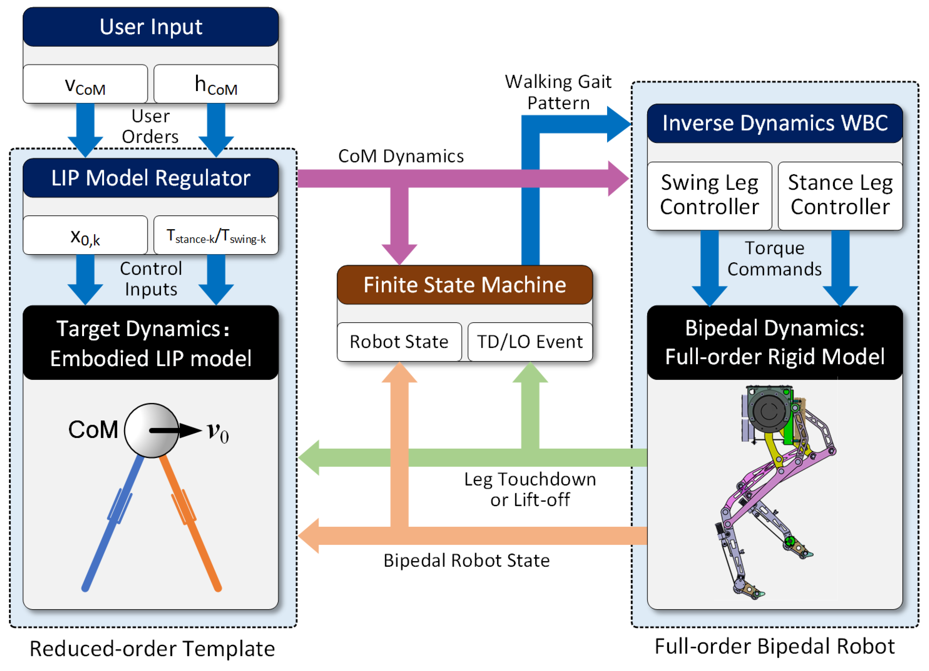
4.3. Whole-Body Control Framework of the Bipedal Robot

Based on the kinematic analysis, dynamic modeling, and swing/stance leg controller design, the whole-body control framework of the bipedal robot is established as shown in Figure 9. Generally, the control framework has two layers, namely, the regulation layer that applies the adjustable LIP model to generate the prescribed trajectory of the CoM, and the joint control layer, which offers individual torque commands via the inverse dynamics-based WBC. The desired walking speed v_CoM and the standing height h_CoM are regarded as the user input from the high-level orders.

In the regulation layer, the LIP model regulator provides the specified CoM’s position together with the swing/stance portion of each gait cycle according to the user’s order collection {v_CoM, h_CoM}. The embodied LIP model, as the target dynamics, evolves by Algorithm 1, resulting in a reactive walking pattern for the bipedal robot. In the joint control layer, the inverse dynamics-based WBC receives the CoM signal from the LIP model and also the walking gait pattern (i.e., swing/stance portion, TD and LO timings). The torque commands for all four actuators coaxially arranged at the hips of the robot are acquired according to the optimal solution of the QP problem (28) and operated in local closed-loop control mode in the hardware. The finite state machine (FSM) is employed to connect the reduced-order template and the full-order bipedal robot. The main task of the FSM is to allocate the swing/stance phase according to the TD/LO events detected from the real robot and transfer the corresponding target dynamics of the LIP model for the bipedal robot. The entire walking stability of the bipedal robot is guaranteed hierarchically via the double-layer architecture of the control framework. On the regulation layer, the deadbeat controller in Algorithm 1 guarantees the trajectory convergence of the CoM on the sagittal plane in a discrete manner from stride to stride. On the joint control layer, the PD-type adjustment of ${\ddot{\mathit{x}}}_{\mathrm{CoM}}^{cmd}$ together with the WBC forces the bipedal robot to reproduce the target dynamics of the LIP model by executing the tracking task.

5. Experiments

5.1. Experimental Setups

The testbed for the bipedal robot prototype is constructed as shown in Figure 10 to evaluate the walking performance. The robot with lateral limiters is arranged on the treadmill. The lateral limiters, made of carbon fiber-reinforced plastic, restrict the robot to walking within the sagittal plane. The lateral limiter mounted on the linear slideway (HIWIN-RG) connects to the upper body of the robot via a pair of passive hinges without interfering with the pitch motion of the robot during the walking test. The treadmill with an adjustable speed range of 0.8~20 km/h and maximal payload of 120 kg is manually manipulated as shown in the local view of Figure 10. In the walking test, the desired speed of the robot is set by the wireless handle via Bluetooth communication to the mini personal computer, as detailed in Section 2.3. Meanwhile, a safe string is applied to suspend the robot in the case of unexpected falling. In most of the experimental period, this safe string is relaxed, which indicates that the fluctuation of the upper body of the robot remains in the admissible region; otherwise, overstretching of the string indicates the walking failure case, wherein falling or stumble emerges. The robot prototype is self-contained, with a portable battery unit that guarantees a power supply for uninterrupted walking for approximate 55 min. The proprioceptive sensory information is synchronously sampled and recorded for post-processing and performance evaluation of the walking test.

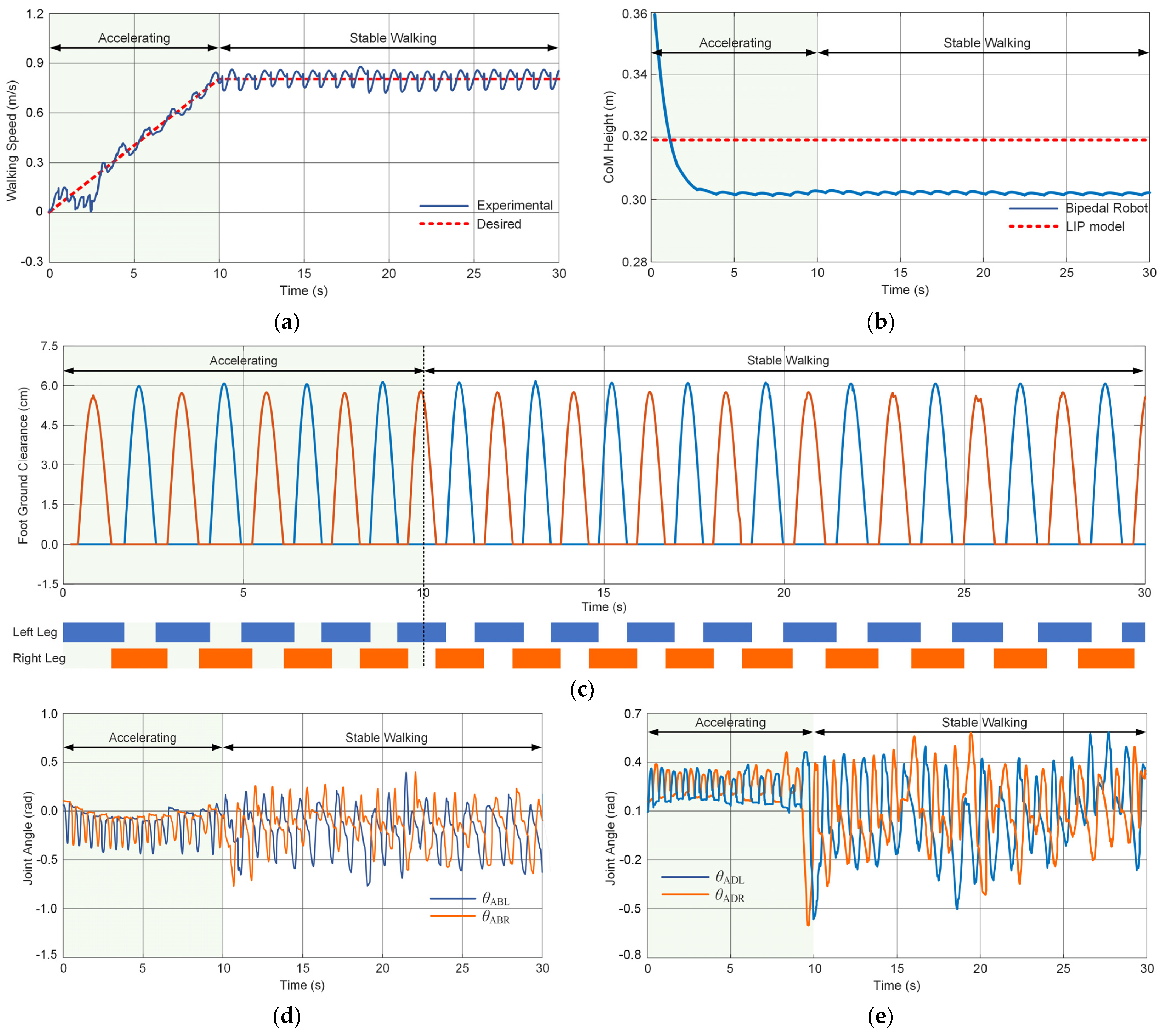
5.2. Stable Walking Test

In the experimental scenario of the walking test, the bipedal robot starts from the rest standing posture as the initial state. The desired speed profile of the robot is a combination of a ramp signal from 0 m/s to 0.8 m/s (lasting 10 s) and a constant signal of 0.8 m/s (lasting 20 s). Figure 11 shows the snapshots of the robot experiencing rest standing, accelerating, and stable walking in chronological sequence. It is clear to observe that the robot exhibits a stable walking pattern during the entire test procedure. The safe string over the upper body of the robot always stays loose, without being strengthened, which implies that the body of the robot can be effectively restricted in a feasible space in both the accelerating stage and the stable walking stage. Figure 11 also indicates the contact foot from individual snapshots, wherein at least one leg is on the ground, which is consistent with the biological observation in Section 2.2.

Figure 12a shows the walking speed of the bipedal robot during the entire test. Although the fluctuation of the body speed is observed in the early steps within 5 s, the robot apparently attains stable walking with the speed variation range [0.74, 0.88] m/s, which validates the effectiveness of the proposed control framework in the bipedal robot. In order to evaluate the walking performance of the LIP-model based control algorithm, we plot the CoM height of the robot in comparison with the height value of the ideal LIP model in Figure 12b. Note that the desired CoM height of the LIP model is set at 0.32 m. The actual height of the robot rapidly converges into the steady state around 0.319 m, with slight oscillation. A consistent height bias exists throughout the walking test. This phenomenon can be explained by the gap (approximately 2 mm when unloaded) between the rolling track and the underlying supporting plate of the treadmill. Therefore, this sinkable moving surface for the foot to step on is regarded as terrain disturbance at the stance phase. Fortunately, the robot performs well from stride to stride during the test. Figure 12c shows the feet ground clearance from both legs and the resultant walking gait patterns in terms of a stick diagram. The ground clearance of individual legs is obtained via the forward kinematics based on the sensory feedback of joint encoders. Figure 12d,e shows the active joint angles of θ_ABL, θ_ABR, θ_ADL, and θ_ADR during the walking test. The full stroke for θ_ABL and θ_ABR is 1.17 rad and 1.16 rad, respectively. These values for θ_ADL and θ_ADR are 1.11 rad and 1.14 rad, respectively. The joint trajectories in Figure 12d,e indicate that all active joints work in a feasible range. Larger joint displacements of the coaxially driven actuators are observed when the robot walks at high speed. The proposed algorithm can successfully manage both legs to execute prescribed swing leg movement as generated by the LIP model-based WBC. Obviously, the resultant walking gait derived from the stick diagram comes into a stable pattern with the duty factor 0.56 for a single leg, which implies that the controller can successfully achieve dynamic walking based on the LIP model.

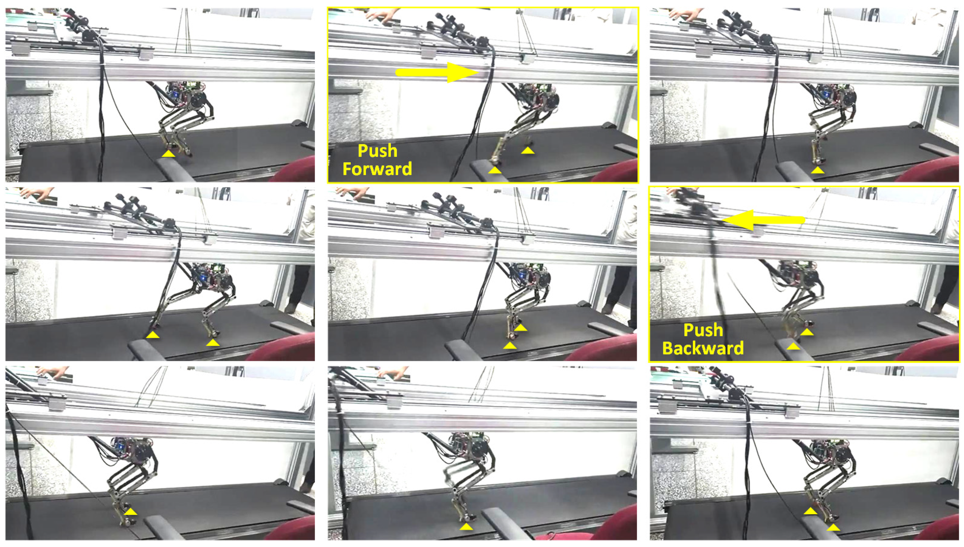
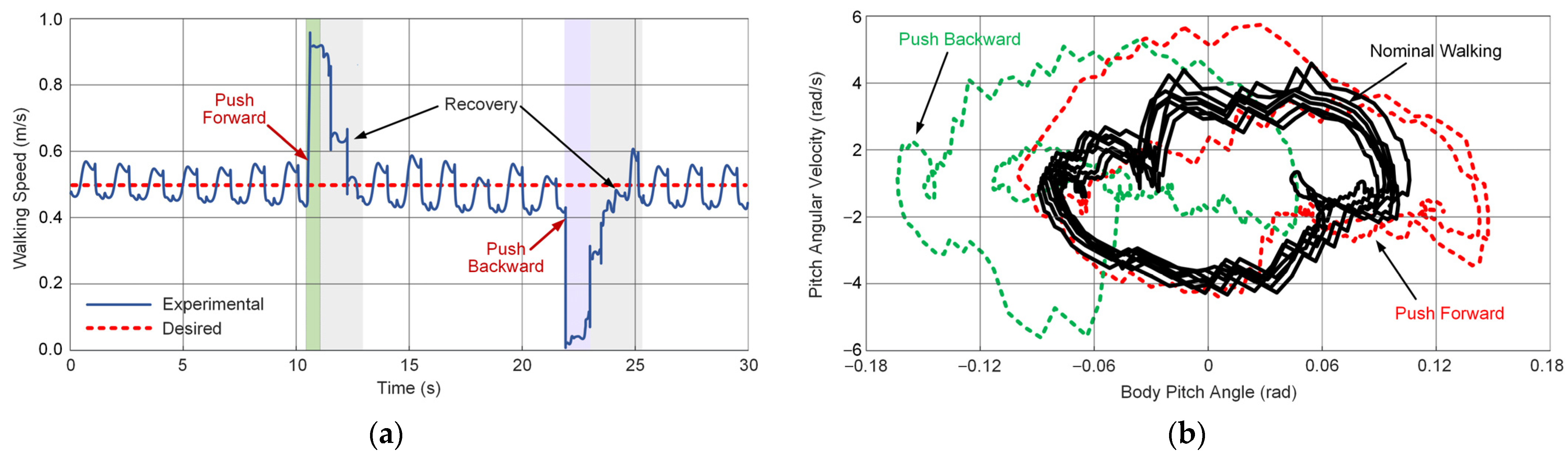
5.3. Push Recovery Test

In the experimental scenario of the push recovery test, the bipedal robot maintains stable walking at a speed of 0.5 m/s. Meanwhile, the rolling track of the treadmill provides reversed smooth movement at the identical rate to guarantee the robot is located at the neutral area of the track. The external disturbance in terms of pushing force is manually imposed on the upper body of the robot from the mechanical coupling on the slideway to the parallel lateral limiters. Pushing forward and backward emerge at T = 10.06 s (applying duration of 1 s) and T = 21.5 s (applying duration of 1.1 s), respectively. Additionally, we remove the safe string hanging over the robot to avoid overshoot scratching. Figure 13 shows the snapshots of the robot experiencing external disturbances and recovering into stable walking. The bipedal robot exhibits satisfactory robustness against these external pushing disturbances on the sagittal plane. When suffering from the sudden drag force to push the body forward and backward, the robot takes no more than four steps to recover and displays a quasi-periodic walking pattern, as expected. Moreover, the passive tendon offers favorable compliance in ameliorating the foot–ground interaction, especially in the presence of external disturbances. No drastic fluctuation of the body is observed during the entire testing procedure.

Figure 14a shows the speed profile of the bipedal robot when facing the external disturbance. It is clear to see that the robot undergoes several adjusting steps toward a normal walking pattern, although a huge velocity disturbance (nearly 92% and 95% for the push forward and backward, respectively) occurs during the gait cycle. The target dynamics of the LIP model are generated with a dead-beat control style such that the discrepancy between the disturbed CoM state S^dis and the desired state S^des is compensated from stride to stride in the coming gait cycles. From the perspective of walking performance, the robot endows robustness against external disturbance in terms of body velocity jump, without recourse to additional high-level motion replanning or control strategies.

In an attempt to investigate the disturbance rejection ability of the robot, we select the body pitch to represent the body posture to create the phase portrait as shown in Figure 14b. Generally, there exists a stable limit cycle, representing the nominal walking in the test. Transient state jumps are observed in cases of pushing forward and backward. The variation of the body pitch is within the range of [−0.07, 0.08] rad for the period of nominal walking during the test. The dashed trajectories show the convergence process of the body posture on the phase plane of the pitch angle. In the experiment, the manual drag force is applied via the interaction between the parallel lateral limiters and the passive spherical hinges mounted on the upper body of the robot. In these circumstances, the equivalent deflection moment is exerted on the robot, since the hinge center does not coincide with the CoM of the robot, which always leads to a sudden perturbation in the pitch angle. This phenomenon can be clearly observed from the dashed trajectories in the push forward and backward cases, in which the transient perturbations of 0.12 rad (lean forward) and 0.13 rad (lean backward) appear. That being said, the proposed control framework shows favorable push recovery capacity to maintain sagittal stable walking without falling down, which showcases the advantage of applying this LIP model-based WBC in the dynamic locomotion control of the bipedal robot.

6. Conclusions

This paper presents the development, modeling, control and experimental validation of a bipedal walking robot with a passive tendon element. The bipedal robot, featuring coaxially actuating at the hip, is equipped with legs in the configuration of the five-bar mechanism. A novel passive artificial tendon is fabricated and integrated in single leg to mimic the functionality of the muscle–tendon complex around the human ankle based on the biomechanical observations. The kinematics of the robot with closed-chain constraint of the single-leg linkages are discussed. The walking control framework is developed based on a double-layer architecture. In the regulation layer, the LIP model with the deadbeat style of parameter adjustment is employed to generate the prescribed trajectory of the CoM. In the joint control layer, the inverse dynamics-based WBC is constructed to transfer the regulation trajectory of the LIP model into the torque commands of individual actuators. The experiments on the bipedal robot prototype are conducted to validate the effectiveness of the proposed control algorithm. The results of the stable walking test on the treadmill demonstrate that the robot with the passive tendon achieves rapid sagittal walking at the speed of 0.8 m/s (nearly twice the leg length/s). The results of the push recovery test showcase the robustness of the robot against external disturbance on the sagittal plane.

Our future work will incorporate the following additions. First, the biologically inspired muscle-tendon complex will be deeply investigated to integrate more elastic tendon-like elements into the leg structure. Second, the bipedal prototype together with the hardware should be upgraded by adding lateral DoFs at the hips, providing the possibility of 3D walking with enhanced foot–ground interactions. Last but not least, the proposed control framework in the double-layer architecture will be evolved by adding learning techniques to handle more challenging locomotory tasks, such as complex agile human-like motion generation, reflex-centered recovery from large disturbances, and traversing complex terrains.

References

1. Raibert, M. Legged Robots That Balance, 1st ed.; The MIT Press: Cambridge, MA, USA, 1986; pp. 2–9. [Google Scholar]
2. Yu, H.; Gao, H.; Ding, L.; Li, M.; Deng, Z.; Liu, G. Gait Generation with Smooth Transition Using CPG-Based Locomotion Control for Hexapod Walking Robot. IEEE Trans. Ind. Electron. 2016, 63, 5488–5500. [Google Scholar] [CrossRef]
3. Hutter, M.; Gehring, C.; Höpflinger, M.; Blösch, M.; Siegwart, R. Toward Combining Speed, Efficiency, Versatility, and Robustness in an Autonomous Quadruped. IEEE Trans. Robot. 2014, 30, 1427–1440. [Google Scholar] [CrossRef]
4. Yi, H.; Xu, Z.; Xin, X.; Zhou, L.; Luo, X. Bio-inspired Leg Design for a Heavy-Duty Hexapod Robot. J. Bionic. Eng. 2022, 19, 975–990. [Google Scholar] [CrossRef]
5. Hurst, J.W.; Rizzi, A.A. Series Compliance for An Efficient Running Gait. IEEE Robot. Autom. Mag. 2008, 15, 42–51. [Google Scholar] [CrossRef]
6. Park, H.W.; Ramezani, A.; Grizzle, J.W. A Finite-State Machine For Accommodating Unexpected Large Ground-Height Variations in Bipedal Robot Walking. IEEE Trans. Robot. 2013, 29, 331–345. [Google Scholar] [CrossRef]
7. Liu, X.; Rossi, A.; Poulakakis, I. A Switchable Parallel Elastic Actuator and Its Application to Leg Design for Running Robots. IEEE/ASME Trans. Mech. 2018, 23, 2681–2692. [Google Scholar] [CrossRef]
8. Yang, T.; Westervelt, E.R.; Schmiedeler, J.P.; Bockbrader, R.A. Design and Control of a Planar Bipedal Robot ERNIE with Parallel Knee Compliance. Auton. Robot. 2008, 25, 317–330. [Google Scholar] [CrossRef]
9. Haeufle, D.F.B.; Taylor, M.D.; Schmitt, S.; Geyer, H. A Clutched Parallel Elastic Actuator Concept: Towards Energy Efficient Powered Legs in Prosthetics and Robotics. In Proceedings of the Fourth IEEE RAS/EMBS International Conference on Biomedical Robotics and Biomechatronics, Roma, Italy, 24–27 June 2012. [Google Scholar]
10. Reher, J.; Ames, A.D. Dynamic Walking: Toward Agile and Efficient Bipedal Robots. Ann. Rev. Contr. Robot. 2021, 4, 535–572. [Google Scholar] [CrossRef]
11. Sreenath, K.; Park, H.W.; Poulakakis, I.; Grizzle, J.W. Embedding Active Force Control within the Compliant Hybrid Zero Dynamics to Achieve Stable, Fast Running on MABEL. Int. J. Robot. Res. 2013, 32, 324–345. [Google Scholar] [CrossRef]
12. Che, J.; Pan, Y.; Yan, W.; Yu, J. Leg Configuration Analysis and Prototype Design of Biped Robot Based on Spring Mass Model. Actuators 2022, 11, 75. [Google Scholar] [CrossRef]
13. Yamamoto, K.; Kamioka, T.; Sugihara, T. Survey on Model-Based Biped Motion Control for Humanoid Robots. Adv. Robotics. 2020, 34, 1353–1369. [Google Scholar] [CrossRef]
14. Yu, H.; Gao, H.; Deng, Z. Toward a Unified Approximate Analytical Representation For Spatially Running Spring-Loaded Inverted Pendulum. IEEE Trans. Robot. 2021, 37, 691–698. [Google Scholar] [CrossRef]
15. Takenaka, T.; Matsumoto, T.; Yoshiike, T. Real Time Motion Generation and Control For Biped Robot-1st Report: Walking Gait Pattern Generation. In Proceedings of the IEEE International Conference on Intelligent Robots and Systems, St. Louis, MO, USA, 10–15 October 2019. [Google Scholar]
16. Geyer, H.; Seyfarth, A.; Blickhan, R. Compliant Leg Behavior Explains Basic Dynamics of Walking and Running. Proc. R. Soc. Lond. B. 2006, 273, 2861–2867. [Google Scholar]
17. Ahmadi, M.; Buehler, M. Controlled Passive Dynamic Running Experiments with the ARL-Monopod II. IEEE Trans. Robot. 2006, 22, 974–986. [Google Scholar] [CrossRef]
18. Hobbelen, D.G.E.; Wisse, M. Swing-Leg Retraction For Limit Cycle Walkers Improves Disturbance Rejection. IEEE Trans. Robot. 2008, 24, 377–389. [Google Scholar] [CrossRef]
19. Posa, M.; Cantu, C.; Tedrake, R. A Direct Method For Trajectory Optimization of Rigid Bodies Through Contact. Int. J. Robot. Res. 2014, 33, 69–81. [Google Scholar] [CrossRef]
20. Saab, L.; Ramos, O.E.; Keith, F.; Mansard, N.; Soueres, P.; Fourquet, J.Y. Dynamic Whole-Body Motion Generation Under Rigid Contacts and Other Unilateral Constraints. IEEE Trans. Robot. 2013, 29, 346–362. [Google Scholar] [CrossRef]
21. Calanca, A.; Fiorini, P. Understanding Environment-Adaptive Force Control of Series Elastic Actuators. IEEE/ASME Trans. Mech. 2018, 23, 413–423. [Google Scholar] [CrossRef]
22. Paine, N.; Oh, S.; Sentis, L. Design and Control Considerations for High-Performance Series Elastic Actuators. IEEE/ASME Trans. Mech. 2014, 19, 1080–1091. [Google Scholar] [CrossRef]
23. Jafari, A.; Tsagarakis, N.; Caldwell, D. A Novel Intrinsically Energy Efficient Actuator with Adjustable stiffness (AwAS). IEEE/ASME Trans. Mech. 2013, 18, 355–365. [Google Scholar] [CrossRef]
24. Mörl, F.; Siebert, T.; Häufle, D. Contraction Dynamics and Function of the Muscle-Tendon Complex Depend On the Muscle Fibre-Tendon Length Ratio: A Simulation Study. Biomech. Model Mechanobiol. 2016, 15, 245–258. [Google Scholar] [CrossRef] [PubMed]
25. Sawicki, G.S.; Robertson, B.D.; Azizi, E.; Roberts, T.J. Timing matters: Tuning the Mechanics of a Muscle-Tendon Unit by Adjusting Stimulation Phase During Cyclic Contractions. J. Exp. Biol. 2015, 218, 3150–3159. [Google Scholar] [CrossRef] [PubMed]
26. Lai, A.; Schache, A.G.; Lin, Y.; Pandy, M.G. Tendon Elastic Strain Energy in the Human Ankle Plantar-Flexors and Its Role with Increased Running Speed. J. Exp. Biol. 2014, 217, 3159–3168. [Google Scholar] [CrossRef] [PubMed]
27. Jackson, R.W.; Dembia, C.L.; Delp, S.L.; Collins, S.H. Muscle-Tendon Mechanics Explain Unexpected Effects of Exoskeleton Assistance On Metabolic Rate During Walking. J. Exp. Biol. 2017, 220, 2082–2095. [Google Scholar] [CrossRef] [PubMed]
28. Sovukluk, S.; Englsberger, J.; Ott, C. Highly Maneuverable Humanoid Running via 3D SLIP+Foot Dynamics. IEEE Robot. Autom. Let. 2024, 9, 1131–1138. [Google Scholar] [CrossRef]
29. Xiong, X.; Ames, A. 3-D Underactuated Bipedal Walking via H-LIP Based Gait Synthesis and Stepping Stabilization. IEEE Trans. Robot. 2022, 38, 2405–2425. [Google Scholar] [CrossRef]
30. Shamsha, A.; Gu, Z.; Warnke, J.; Zhao, Y.; Hutchinson, S. Integrated Task and Motion Planning For Safe Legged Navigation in Patially Observable Environments. IEEE Trans. Robot. 2023, 39, 4913–4934. [Google Scholar] [CrossRef]
31. Kajita, S.; Kanehiro, F.; Kaneko, K.; Yokoi, K.; Hirukawa, H. The 3D linear Inverted Pendulum Model: A Simple Modeling For A Biped Walking Pattern Generation. In Proceedings of the IEEE International Conference on Intelligent Robots and Systems, Maui, HI, USA, 29 October–3 November 2001. [Google Scholar]
32. Ott, C.; Dietrich, A.; Schäffer, A.A. Prioritized multi-task compliance control of redundant manipulators. Automatica 2015, 53, 416–423. [Google Scholar] [CrossRef]
Figure 1. General description of the self-developed bipedal robot: (a) CAD model; (b) physical prototype with basic components.
Actuators 13 00240 g001
Figure 2. Biomechanics observations and anatomy findings: (a) walking snapshots of human subject; (b) skeletal structure of the human foot; (c) illustration of contact stages in stance phase of the human foot. The arrows indicate the direction of the ground reaction force at different stance stages.
Actuators 13 00240 g002
Figure 3. Details of the shank and foot with the passive tendon. The passive tendon is fabricated by emulsion, with a local view of the physical prototype. Key components and assembly of the elastic elements in the shank–foot complex are shown via the CAD model.
Actuators 13 00240 g003
Figure 4. Architecture of the electrical system of the bipedal robot.
Actuators 13 00240 g004
Figure 5. Coordinates and linkage description of the five-bar mechanism of single leg.
Actuators 13 00240 g005
Figure 6. Division and illustration of the chains in the five-bar mechanism of the single leg.
Actuators 13 00240 g006
Figure 7. Illustration and division of the LIP model-based walking gait pattern. Shaded regions indicate the double support phase.
Actuators 13 00240 g007
Figure 8. Swing leg trajectory on the sagittal plane.
Actuators 13 00240 g008
Figure 9. Architecture of the LIP model-based whole-body control framework.
Actuators 13 00240 g009
Figure 10. Experimental setups for the bipedal walking robot: (a) CAD model of the experimental scenario; (b) arrangement of the bipedal robot at rest standing posture of initial state. Local view shows the speed controller of the treadmill.
Actuators 13 00240 g010
Figure 11. Snapshots of the bipedal robot achieving stable walking gait pattern. The key frames are highlighted with the locomotion stages the robot enters. The leg in stance during the gait cycle is identified in yellow.
Actuators 13 00240 g011
Figure 12. Experimental results of the bipedal robot in the stable walking test: (a) walking speed of the robot; (b) CoM height of the robot; (c) feet ground clearance and the resultant walking gait pattern illustrated by a stick diagram. Shaded region represents stance phase; (d) active joint angles for θABL and θABR; (e) active joint angles for θADL and θADR.
Actuators 13 00240 g012
Figure 13. Snapshots of the bipedal robot achieving push recovery under external disturbance. The key frames are highlighted with external push illustrations. The leg in stance during the gait cycle is identified in yellow.
Actuators 13 00240 g013
Figure 14. Experimental results of the bipedal robot in the push recovery test: (a) walking speed of the robot; (b) phase portrait of the body posture during the push recovery test.
Actuators 13 00240 g014