Abstract
This paper introduces a current control method for permanent magnet synchronous motors (PMSMs) using a disturbance sliding mode observer (DSMO) in conjunction with a linear quadratic regulator (LQR). This approach enhances control performance, streamlines the tuning of controller parameters, and offers robust optimal control that is resistant to system disturbances. The LQR controller based on state feedback is advantageous for its simplicity in parameter adjustment and achieving an optimal control effect easily under specific performance indicators. It is suitable for the optimal control of strong linear systems that can be accurately modeled. However, most practical systems are difficult to model accurately, and the time-varying system parameters and existing nonlinearity limit the engineering application of LQR. In the PMSM current control loop, there is strong nonlinear disturbance manifesting as the nonlinearity of its dynamic model. Additionally, substantial noise and variations in system parameters within actual motor circuits hinder the linear quadratic regulator from attaining optimal performance. A disturbance sliding mode observer is proposed to enhance the LQR controller, enabling superior performance in nonlinear current loop control. Simulation and actual hardware experiments were conducted to verify the performance and robustness of the control scheme proposed in this paper. Compared with the widely used PI controller in engineering and sliding mode control (SMC) specialising in disturbance rejection, it offers the advantage of straightforward parameter tuning and can swiftly achieve the robust and optimal control performance that engineers prioritize.
1. Introduction
Thanks to the development of rare earth permanent magnet processing technology, humans can manufacture high magnetic energy product permanent magnets, which can make the motor smaller and lighter, while providing a stronger magnetic field and higher efficiency [1]. This has made permanent magnet synchronous motors the preferred solution for high-precision servo control applications in recent years.
Utilizing the decoupling of the flux and torque control scheme proposed by Park, an engineer from Siemens, and a space vector pulse width modulation (SVPWM) drive control scheme with smaller harmonic level, PMSMs can achieve excellent performance. Therefore, they are widely used in high-precision servo direct drive control [2] and precision measurement applications, for instance, in camera remote sensing stabilization platform systems [3]. In the axial servo control of the above systems, the motor current loop is the innermost loop, and the performance of its controller directly determines the performance level of the entire servo system [4,5,6]. Developing a robust and user-friendly optimal controller for the current loop is crucial for designing high-precision direct-drive servo systems with permanent magnet synchronous motors.
The challenges faced by PMSM current control in practical design mainly include the following points. The first issue is the inaccuracy of the motor model parameters, as engineers typically only obtain nominal motor parameters with significant error. The second challenge is that the motor parameters will change with the operating conditions. Even if accurate parameters of the motor are obtained through various efforts, they will only be accurate under certain operating condition. The motor parameters will change with the aging of its own components, changes in the surrounding working environment, and even after each startup. The third challenge is the limitation of computing resources and speed. In practical products, embedded current controllers usually operate at high control frequencies, usually above 10 kHz. Restricted computing resources limit the complexity of the control algorithm. Actual high-precision servo systems have higher requirements for control performance and long-term working accuracy stability of the motor actuator. However, most PMSM current loop control algorithms are in the laboratory validation stage. In other words, in a good working environment PMSMs can achieve considerable accuracy, but in other demanding working environments, their actual usage accuracy will significantly decrease. In order to design high-performance current controllers, many scholars have adopted various control schemes and algorithms, including modified classical PI control, current prediction control, data-driven neural network assisted control, and optimization control, such as LQR and MPC control, sliding mode control and so on. Each scheme presents a unique constellation of merits and demerits.
Many scholars have focused on studying how to model and calibrate the various parameters and errors of the motor in order to obtain as accurate prior information as possible [7]. There are also online estimators designed for a certain parameter to obtain real-time estimates. In references [8,9,10,11], offline or a combination of offline and online methods are used to identify the various parameters of the motor. The method is relatively complex or computationally intensive, and the calibrated parameters often change when the working environment changes. References [12,13,14] use online estimation methods to estimate certain parameters of the motor, such as coil resistance, inductance, etc. In order to improving the effectiveness and robustness of the PMSM controller, references [15,16] use a Kalman filter and extended Kalman filter to estimate the magnet flux ripple or demagnetization caused by the high operation temperature, or a stator winding current impulse and the nonlinearity of a voltage-source inverter, respectively. In reference [17], a method based on an unscented Kalman filter (UKF) algorithm is proposed to estimate the permanent magnet flux linkage by taking the inverter dead-time voltage error into consideration. Although the corresponding parameter changes can be estimated in real time, it is difficult to directly use the estimated parameters from the control law designed based on nominal parameter models. PI controllers that are widely used in practical engineering are like this. In the design stage, the initial values of the controller’s relevant parameters can be determined based on accurate calibration parameters, and then adjusted through actual testing. The control law is fixed. When the motor parameters change or the working conditions change, it is difficult to ensure that the control performance does not decline. Consequently, to circumvent the degradation of the performance of a well-crafted control law in actual applications, the comprehensive estimation of various disparities, as well as internal and external disturbances within the control loop, can augment the system’s robustness. References [18,19,20] used a Luenberger disturbance observer to cope with the divergences caused by motor parameter mismatch, magnetic saturation, cross-coupling, and other factors, such as internal unmodeled and external unknown interference during motor operation, to improve the dynamic performance and parameter robustness of deadbeat predictive current control. Aiming at the deterioration of control precision caused by unknown lumped disturbances that exist in a control system, a nonlinear disturbance observer is devised to estimate and further reject disturbance in reference [21]. Moreover, in order to improve the anti-interference capability of the system during operation, a second-order nonlinear disturbance observer model is developed, and the robustness of the system is improved by combining the model with linear sliding mode control in reference [22].
Various current prediction control schemes mainly use established models to predict the current, compensating for some uncertainties in the system through the error between the actual current measurement values and the predicted values [23]. However, in the algorithm design process, there is usually a lack of consideration for actual current sensor noise. The article [24] adopts predictive control to improve the deadbeat control. Compared with the traditional deadbeat controller, its predictive structure adds a numerical integration term to provide robustness to the parameter uncertainty and unmodeled dynamics. This integrator provides indirect disturbance rejection robustness and insufficient disturbance suppression speed. Reference [25] analyzed the impact of different parameter mismatches on system stability and current tracking error, and introduced corresponding compensation mechanisms through robust predictive current control strategies, effectively improving the system’s robustness to parameter changes. Reference [26] directly uses the gradient descent method based on the current results to estimate the total disturbance. This method is simple and easy to implement, but it also does not consider the noise problem of actual current sensors. Moreover, the parameter adjustment of the PI controller used is very time-consuming and labor-intensive, making it difficult to achieve the optimal control goal.
With the popularity of artificial intelligence research, neural network (NN) control has once again been used in the design of PMSM current loop controllers, also known as data-driven. This approach can extract information about the controlled object using actual data. However, due to the difficulty of obtaining training data to cover actual operating conditions, the performance of the controller is unstable. In addition, network training and deployment on actual controllers are time-consuming and labor-intensive, which is not conducive to large-scale use in engineering. Reference [27] proposes an observer scheme based on NN to estimate the back electromotive force (BEMF) for current loop control without position sensors. Reference [28] develops a neural network-based vector controller to overcome the problem of inaccurate decoupling in traditional proportional integral (PI)-based vector control methods
Compared to black box solutions based on neural networks, the optimal control scheme has been favored by many researchers and engineers in recent years, including LQR and MPC [29]. These optimal control schemes are usually based on the design of the optimal control law based on the model, and the performance of the controller is limited by the accuracy of the model parameters. In reference [30], an internal input model was introduced to a control algorithm in order to eliminate the steady state speed error caused by the step reference speed as well as load torque variations. Reference [31] considers that there are always unmodeled dynamics in actual systems, so model-based control methods cannot guarantee accurate output results in all situations. A data-driven LQR control method based on Markov is proposed, which uses estimation of Markov parameters and an extended observability matrix to obtain the optimal feedback control gain without explicitly knowing the system’s dynamic equations, which does not rely on an accurate mathematical model. However, the input and output data used in this method have difficulty covering the actual operating conditions of the system. Model predictive control is an online real-time optimization control scheme used to handle complex optimization control problems through rolling optimization and the ability to handle multiple constraints. In reference [32], an optimization approach to suppress torque disturbance caused by magnetic flux distortion in PMSM is adopted, but the impact of other parameter disturbance on torque spike fluctuation is not considered. In reference [33], a Finite Control Set Modulation Model Predictive Control (FCS-M2PC) is applied to improve the utilization of the PMSM DC bus voltage and reduce the voltage vector tracking error. In reference [34], an improved MPC algorithm was applied to PMSM current loop control. This algorithm selects the optimal voltage vector based on the current trajectory circle rather than the cost function, which can effectively reduce torque fluctuations and current harmonics in a PMSM drive. Reference [35] proposes an improved MPC based on the elimination of current prediction errors, overcoming the problem of parameter mismatch, and enhancing the control performance of the PMSM system. The MPC control algorithm is known for its online optimization and represents a very promising direction for the development of optimization control. However, currently, the MPC algorithm has a large computational load and is difficult to deploy and achieve high control frequencies on embedded controllers. In addition, its optimal solution may fail, which limits its application in high bandwidth current loop control schemes. Compared to traditional QR regulators, they can achieve optimal control in the context of the target, but without the aforementioned drawbacks of MPC, and are an optimal control method suitable for engineering applications. The main challenge faced by traditional QR regulators is the difficulty in obtaining an accurate mathematical model of the controlled object.
An LQR method based on a disturbance sliding mode observer is proposed in this paper to address the challenges faced by LQR in PMSM current loop design and the practical engineering application requirements. The uncertainty of various parameters, changes in motor state, and unmodeled parts of the PMSM motor are classified as total disturbance, and a system dynamics equation containing disturbances is derived. An SMO is used to estimate the real-time disturbance in the current loop in order to improve the control performance of the traditional current LQR used for PMSM.
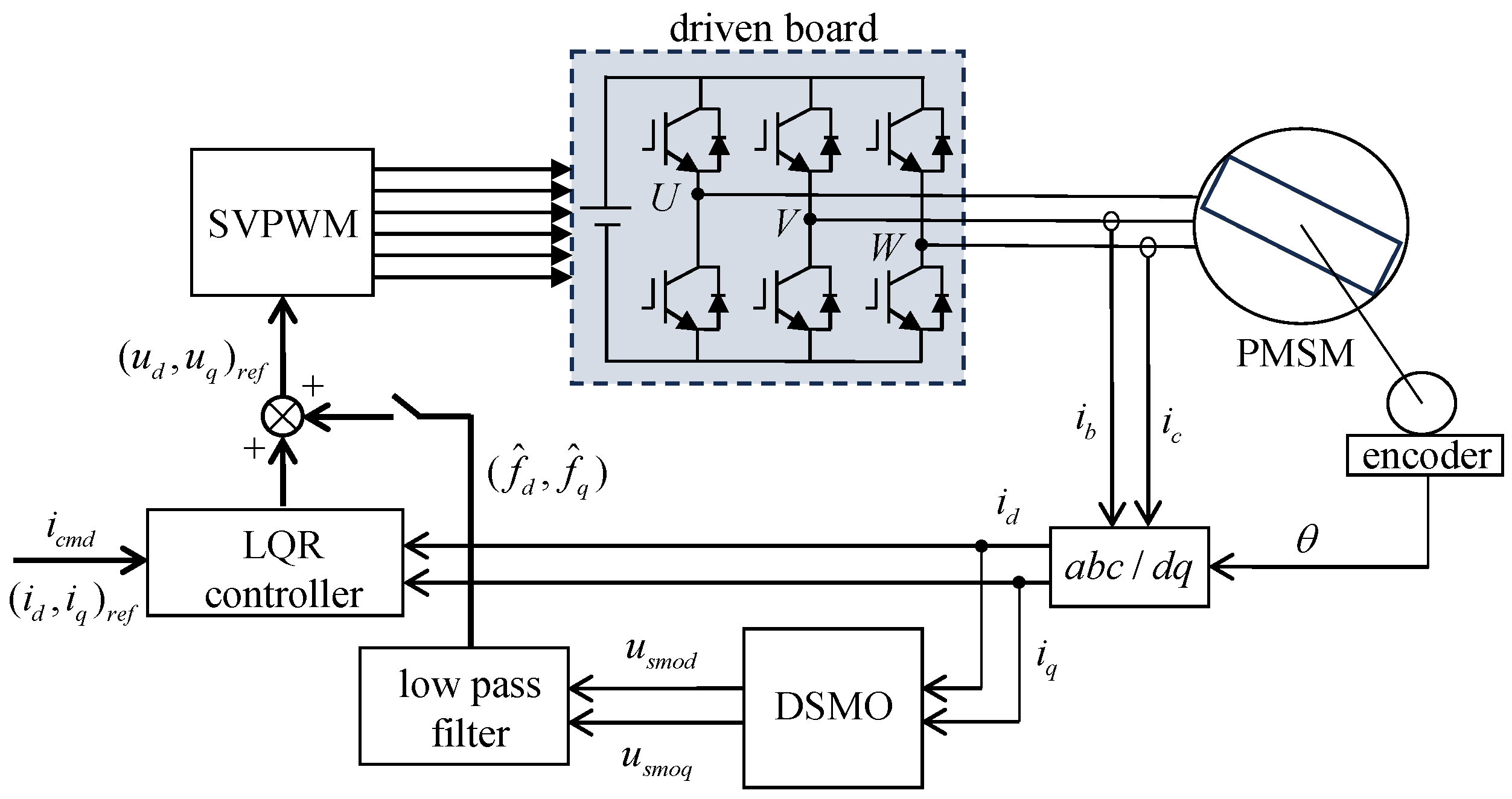
The proposed control scheme base on a disturbance observer is shown in Figure 1.
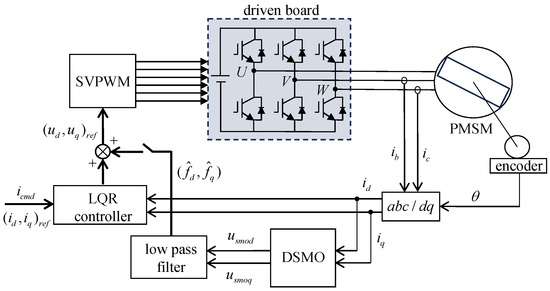
Figure 1.
Current loop control scheme based on a disturbance sliding mode observer.
The remainder of this paper is organized as follows: In Section 2, the PMSM current loop equations with disturbance are established and the disturbance terms are analyzed. In Section 3, the disturbance and system state variable observer based on SMO is designed. Furthermore, the stability analysis of DSMO is conducted and the parameter selection criteria for convergence are derived. Subsequently, a current LQR tracking controller is designed based on DSMO in Section 4. And in Section 5, simulation and experimental verification are conducted to demonstrate the effectiveness of the proposed approach. The Section 6 provides a summary of the work in this paper.
2. Modeling of PMSM Current Loop with Disturbance
The magnetic linkage equation of PMSM in the dq-axis coordinate system in the FOC scheme is as follows:
where is the permanent magnet flux linkage; , represent the -axis flux linkage; , is the -axis inductance; and , is the current in the -axis, respectively.
The voltage equation under the -axis is
where , respectively, represent the voltage below the -axis; is the winding resistance; is the electrical angular velocity; and its relationship with the mechanical angular velocity is . The electromagnetic torque equation under the -axis is
where is the electromagnetic torque. By combining Equations (1) and (2), it can be concluded that the ideal current differential equation can be expressed as
In an actual working environment, the hardware parameters of PMSMs, such as the resistance and inductance of the armature winding, as well as the magnetic flux of the permanent magnet, will inevitably vary with changes in the environment, each time the motor starts, the working state, and the operating time.
In this paper, and are used to represent the uncertain disturbances of the motor parameters relative to the calibration value.
Considering the uncertain disturbance caused by the resistance based on the calibration value, according to Equation (4), the corresponding disturbance in the current loop can be expressed as:
Similarly, given the uncertain disturbance of the -axis inductance , the new balance equation after introducing the inductance parameter disturbance is as follows:
According to the circuit principle and Formulas (5) and (6), the following equation can be obtained:
In addition, the uncertain perturbation of the permanent magnet flux and the inductance variation will also cause disturbance to the -axis flux in the current equation. The calculation model of the flux under the disturbance -axis is:
where , represent the disturbance of the permanent magnet flux in the axis direction and the distortion angle in the direction of the permanent magnet flux, which is usually a small angle.
Finally, the PMSM current loop dynamic equation considering hardware parameter perturbation is established as
where and represent the disturbance below the -axis, and and represent the unmodeled disturbance factors that have not been considered.
The disturbance term in the above established model contains various influencing factors, such as the parameter uncertain perturbation, the changing back electromotive force, as well as unmodeled parts, including nonlinear and time-varying influencing factors, which makes it difficult to design a controller based on the classical linear model. Therefore, a disturbance estimator based on sliding mode control to estimate the total disturbance in the system in real time is designed in this paper. And equivalent compensation is added to the control input in the current loop to eliminate disturbance in a feedforward manner.
3. Design of Disturbance Sliding Mode Observer
3.1. Disturbance Observer Equation
To estimate the disturbance term in the actual current control loop, the system equation for constructing a sliding mode observer is as follows:
where and represent the estimated values of the PMSM’s -axis currents by the sliding mode observer, and , respectively, represent the actual input control effort of the observed motor, and , respectively, represent the error feedback correction of the -axis in the dynamic model of the sliding mode observer, and the other parameters are the nominal argumentations of the motor. And the sliding mode function used in SMO is selected as
where , , , , satisfy the Hurwitz criterion. The feedback control law designed subsequently in the sliding mode observer can ensure that returns to zero, i.e., and its integration get to zero. Upon achieving the aforementioned control objective, the convergence of the observer is realized.
So the derivative of the sliding function is:
By expanding the derivative function (13) of the sliding surface based on the dynamic Equation (11) of SMO, we have:
The exponential convergence law is chosen in this paper to reach the sliding mode surface. It is shown as follows:
where and are the components of , respectively. , and , are all greater than 0.
The feedback correction control law shown in Equation (16) for the sliding mode observer can be obtained by combining the two Equations (14) and (15). In other words, adjusting the observer in accordance with this derived control law enables the state to converge exponentially to the system’s state variables.
Once the observer has converged, it implies that and approach zero, which means that the control efforts applied to the observer are equivalent to the disturbances within the system, thereby also achieving an estimation of the disturbances in the control loop.
3.2. Stability Analysis and Observer Tuning
Due to the presence of unknown disturbances in the feedback control law of the sliding mode observer mentioned above, its upper and lower bounds can be estimated in practical applications based on its expression by Equation (8) using actual system parameters and operating conditions. Then, the convergence of the sliding mode observer can be ensured by designing the parameters , , and in the feedback control law. Assuming that the maximum disturbance values of the estimated -axis are and , respectively, the feedback correction law of the sliding mode observer is:
where and represent the actual control efforts used for the sliding mode observer because the disturbances cannot be accurately known.
Taking the -axis as an example for analysis, in order to ensure the stability of the sliding mode observer, the Lyapunov function is taken as , which is a positive definite function. And its derivative is .
By substituting into in , which is the component of shown in Equation (14), we can obtain the following equation:
Substituting Equation (18) into Equation , we obtain:
The first item on the right , if only can be guaranteed, and then can be achieved. Because the second term on the right-hand side is always negative, once the aforementioned condition is met, its absolute value is always greater than that of the third term . Therefore, regardless of the sign of the third term, it ensures that is negative. According to Lyapunov stability theory, the observer is convergent. Similarly, for the q-axis, it is necessary to satisfy the condition to ensure the convergence of the sliding mode observer. In other words, the sliding mode observer will converge to the sliding surface. At this point, the observation error between the observer and the actual current is 0, and the feedback correction of the sliding mode observer is equal to the disturbance of each axis in a manner similar to PWM modulation. By using a low-pass filter, the disturbance of the corresponding axis can be obtained.
A flowchart of the disturbance sliding mode observer algorithm is shown as Algorithm 1:
| Algorithm 1 Disturbance Estimation Based on Sliding Mode Observer |
|
4. Design of LQR
Real-time estimation and compensation can be achieved through a sliding mode disturbance estimator. When the disturbance observer converges quickly, feedforward control is introduced, which is shown as:
For , , are always desired, i.e., tracking control command is the objective of the actual control loop.
New state variables are taken as:
Because of the fact that the current loop is the innermost loop, its control frequency is usually more than 10 times that of the outer speed loop. It can be considered as a constant here, and after transformation, it is shown as follows:
Substituting the system state:
where , .
The state feedback is shown as:
Substituting the above state feedback into the system control equation:
where .
Select the cost function:
Thus, the standard form of the LQR problem is obtained and the design of the controller is completed. By adjusting the weights of the matrices and , it is relatively easy to adjust the performance that the controller focuses on.
5. Evaluation Results and Discussion
5.1. Simulation Protocol
In order to verify the effectiveness of the proposed algorithm, computer simulation experiments were conducted. In the Simulink environment, a simulation environment for PMSM was built using simscape multi-domain joint simulation. The parameters of the PMSM are shown in Table 1.

Table 1.
The true parameters of PMSM used in the simulation.
The cntrol simulation system sampling time is 0.0001 s. The amplitude of the current noise power spectral density (PSD) is set to 0.02 × 0.02 × 0.0001, and the amplitude of the angular velocity noise PSD is set to 0.01 × 0.01 × 0.0001.
The design of the sliding mode observer and LQR controller is carried out using parameters with an error of about 15% to 25% from the true values of the PMSM parameters in order to simulate the error that always exists in the nominal parameters. The nominal parameters used are shown in Table 2.
Table 2.
The nominal parameters of PMSM used for algorithem design.
5.2. Simulation Results and Discussion
PI control can usually achieve good results and high reliability, and is easy to use, so it is widely used in practical engineering. This paper conducted comparative experiments with the classical PI controller to verify the LQR control effect of the designed disturbance sliding mode observer. The parameter selection of the PI controller is aggressive, with the Kp parameter set to 2.0 and the Ki parameter set to 2000.0. The simulation experiment results are as follows:
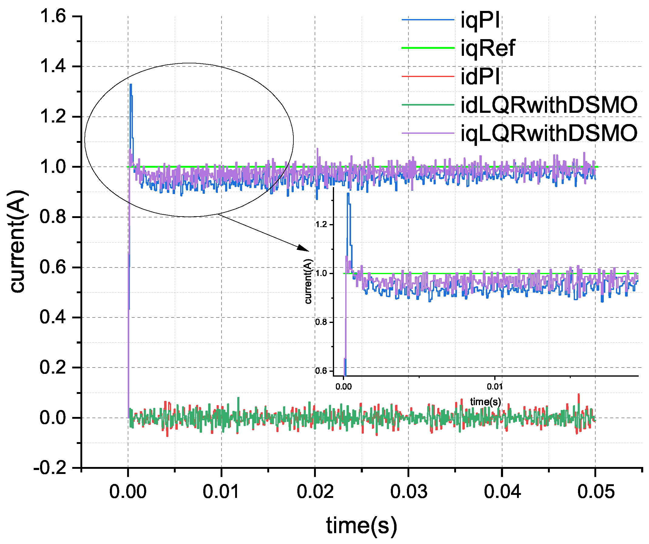
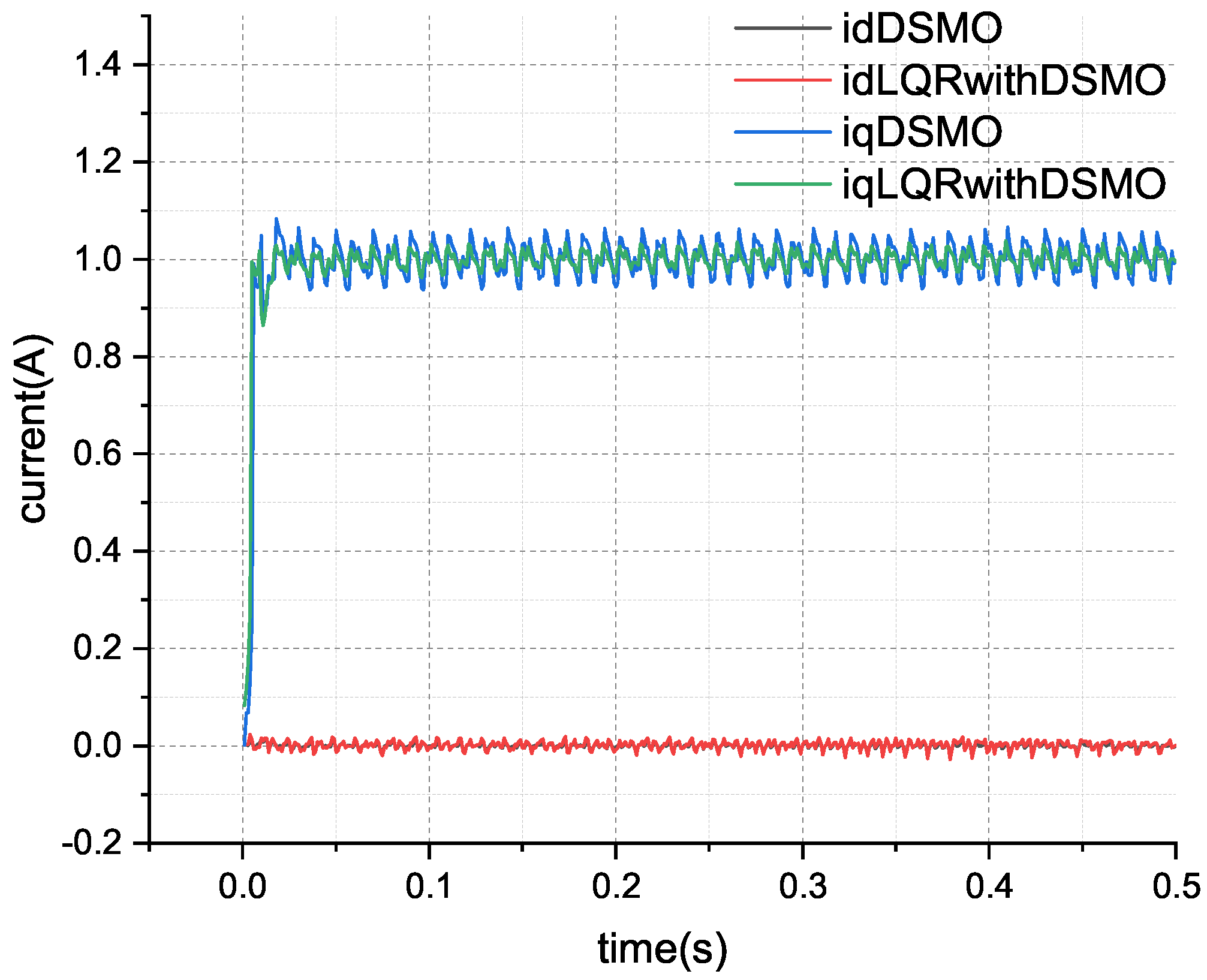
Setting the q-axis command current of the current loop (iqRef in Figure 2) to 1.0 ampere and the d-axis command current to 0.0 ampere, the current tracking effect of the PI controller and the LQR based on DSMO are compared. The step response simulation test results are shown in Figure 2 and Figure 3.
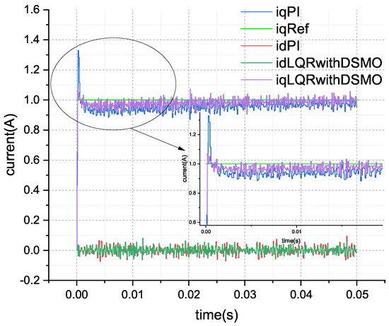
Figure 2.
Comparison diagram of step response control effects of the two schemes.

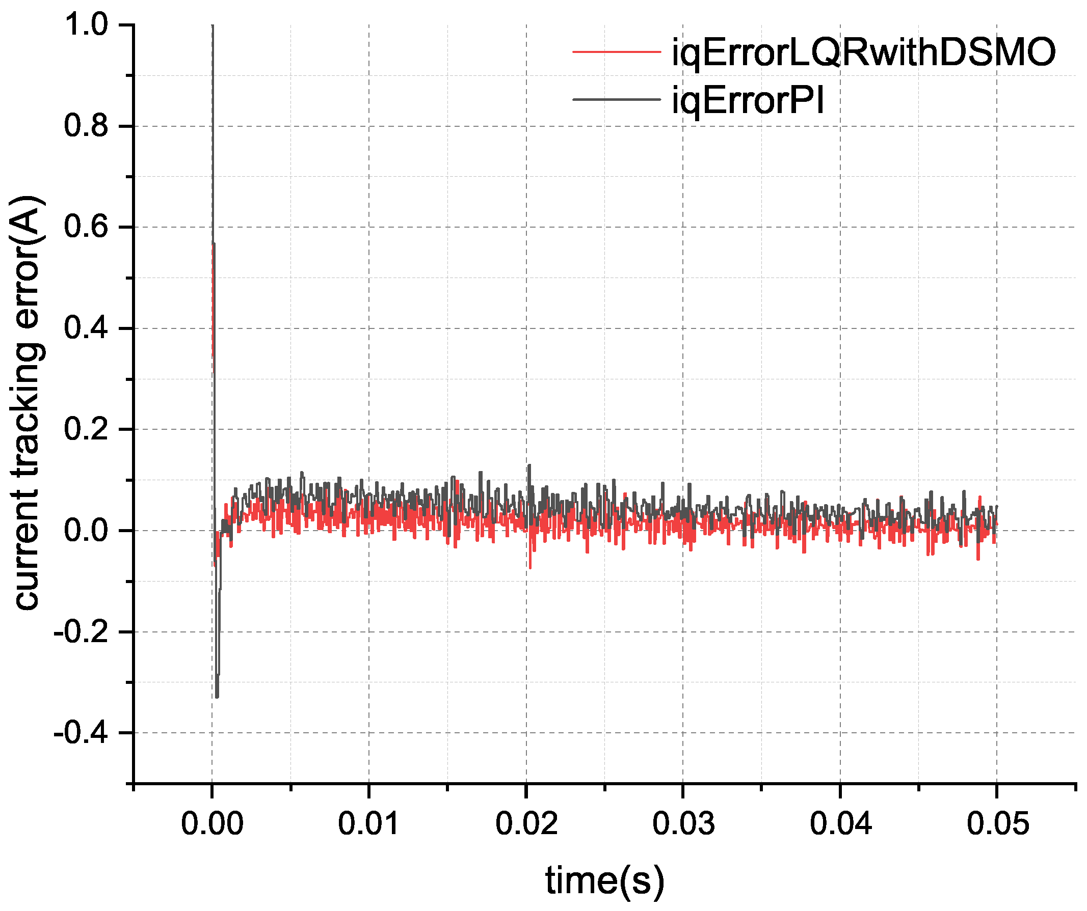
Figure 3.
Comparison diagram of current tracking error of the two schemes.
From Figure 2 and Figure 3, it can be seen that when the current command suddenly changes, the current of both schemes can quickly rise to the reference value of the command, indicating that the Kp parameter setting of the PI controller is relatively aggressive. However, there is a significant control error in the subsequent PI control, which gradually stabilizes at the reference value over time. Although there is some tracking deviation with the LQR control scheme based on DSMO, it maintains a good control effect. Based on the theoretical analysis in the Section 2, it can be seen that the disturbance generated during the operation of the motor current loop is the reason for the control error. Although the integral effect in the PI controller has the ability to resist disturbances, the simulated Ki parameter set here is 2000.0, which is obviously more aggressive and can lead to instability in actual hardware motor control. However, it still cannot effectively suppress disturbances in the circuit. Compared to this, the disturbance feedforward scheme based on a sliding mode observer proposed in this paper shows better control performance.
Figure 3 is a comparison of the current tracking error results between the scheme proposed by this paper and the classic PI scheme.
By calculating the root mean square error (RMSE) of the current, the RMSE of the classical PI controller is 0.0695 A, and the root mean square error of the LQR current control based on a disturbance sliding mode observer is 0.0489 A, resulting in an improvement in the control accuracy of approximately 29.64%. Clearly, the control scheme proposed in this paper has achieved the expected results.
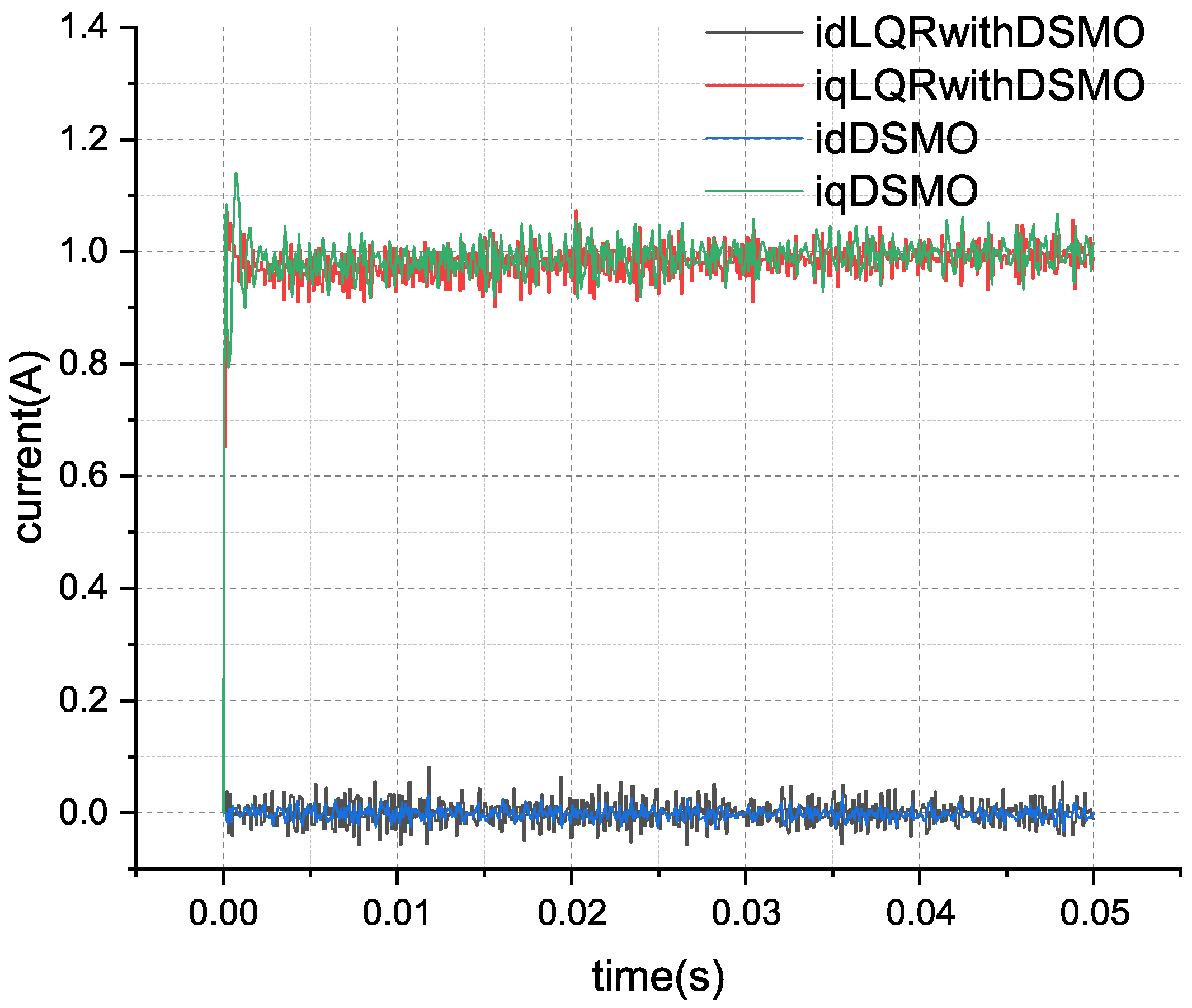
The current tracking effect of the disturbance sliding mode observer is a very intuitive criterion for evaluating the convergence of the observer. The results of the current value estimated by a sliding mode observer and the actual current value are shown in Figure 4.
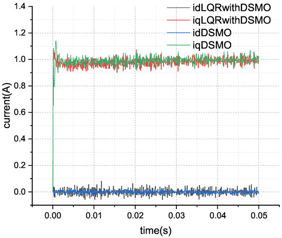
Figure 4.
Estimation and convergence result of the sliding mode observer.
In Figure 4, the red line represents the actual q-axis current value, and the green line represents the q-axis current value of the sliding mode observer. It can be seen that the sliding mode observer can quickly converge to the tracked q-axis current, and the same is true for the d-axis. This also verifies the correctness of the convergence analysis of the observer in the Section 3.
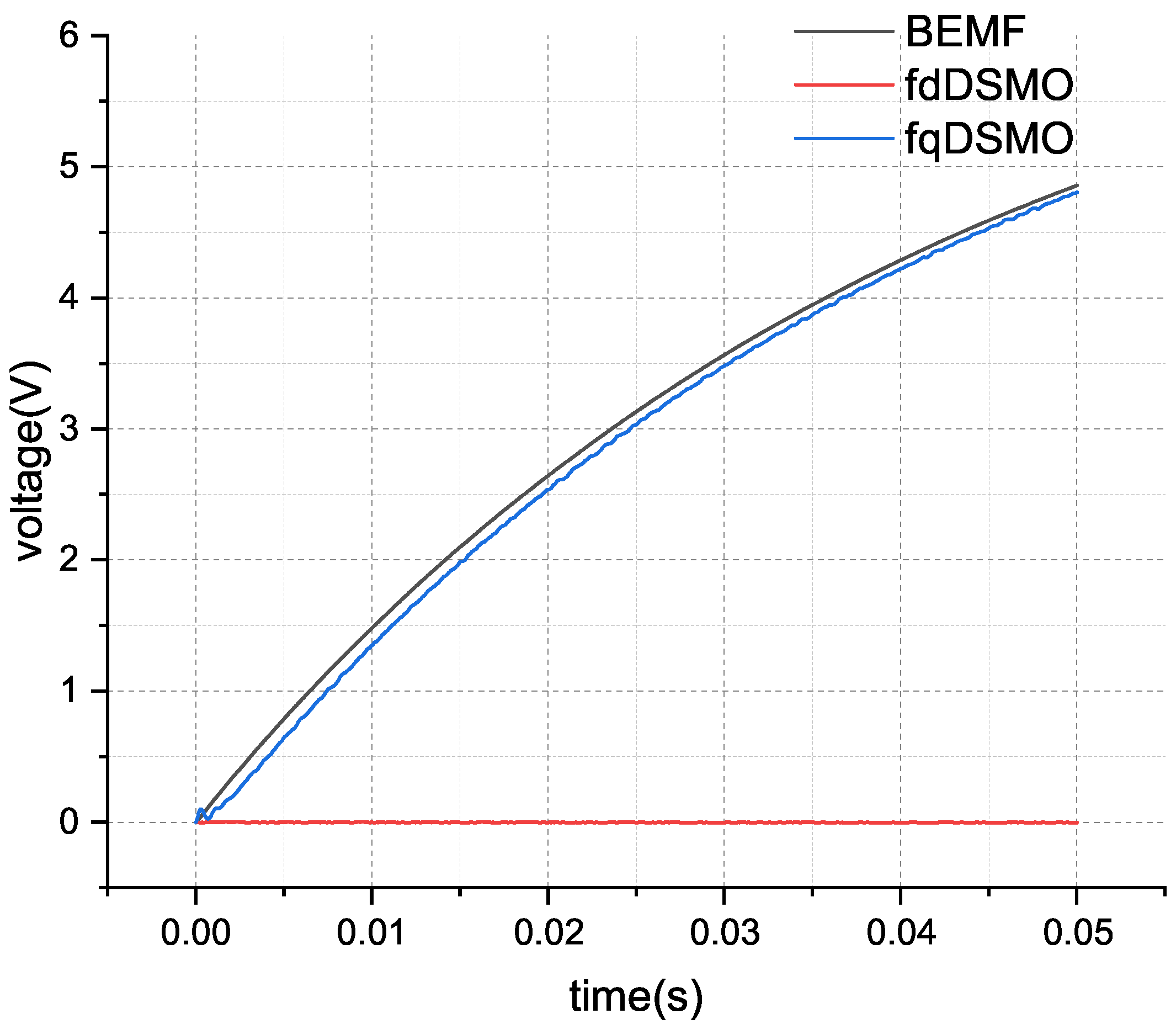
The estimation of disturbances in the circuit by the sliding mode observer is shown in Figure 5.
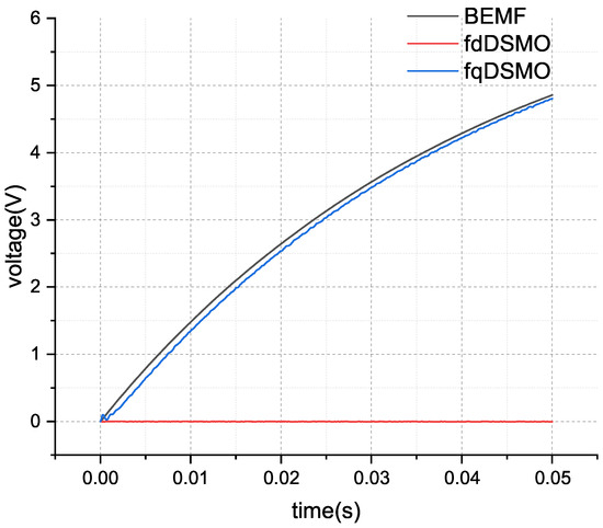
Figure 5.
Estimation result of the disturbance in the -axis by the sliding mode observer.
Under simulation conditions, the back electromotive force term in the circuit can be accurately obtained, as shown in the black curve in the figure. According to the theoretical analysis of the disturbance model Equation (8), it can be seen that this is a larger part of the q-axis disturbance. From the simulation results, it can also be seen that the variation trend of the q-axis disturbance (blue curve) is the same as its main part of the back electromotive force, indicating the effectiveness of the disturbance estimator design.
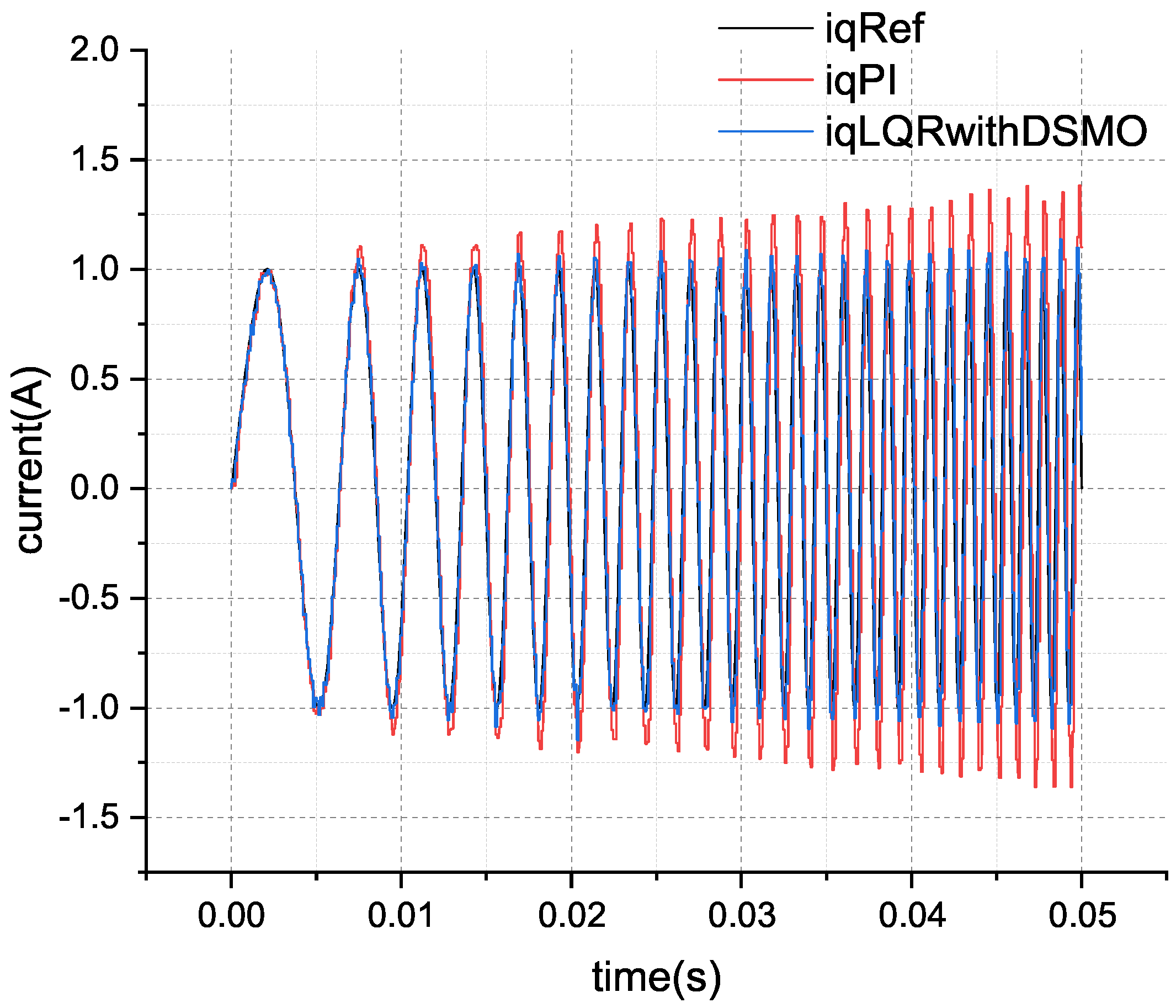
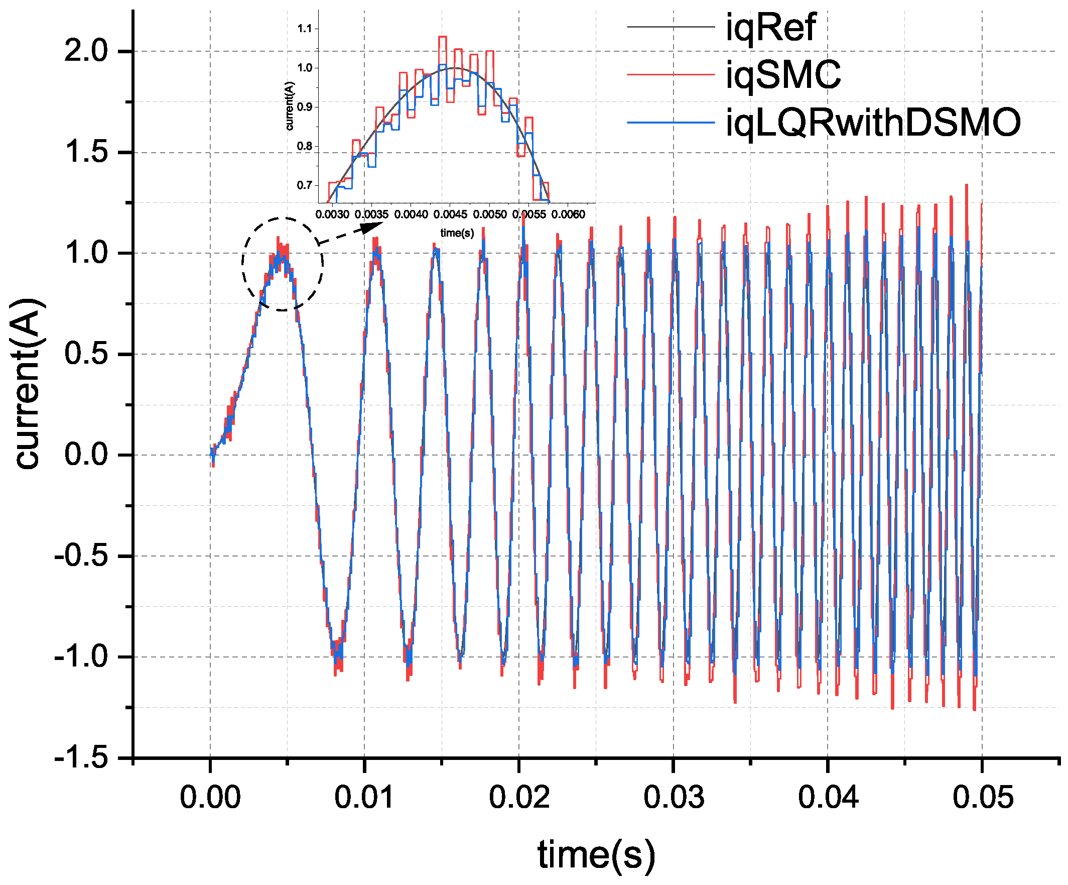
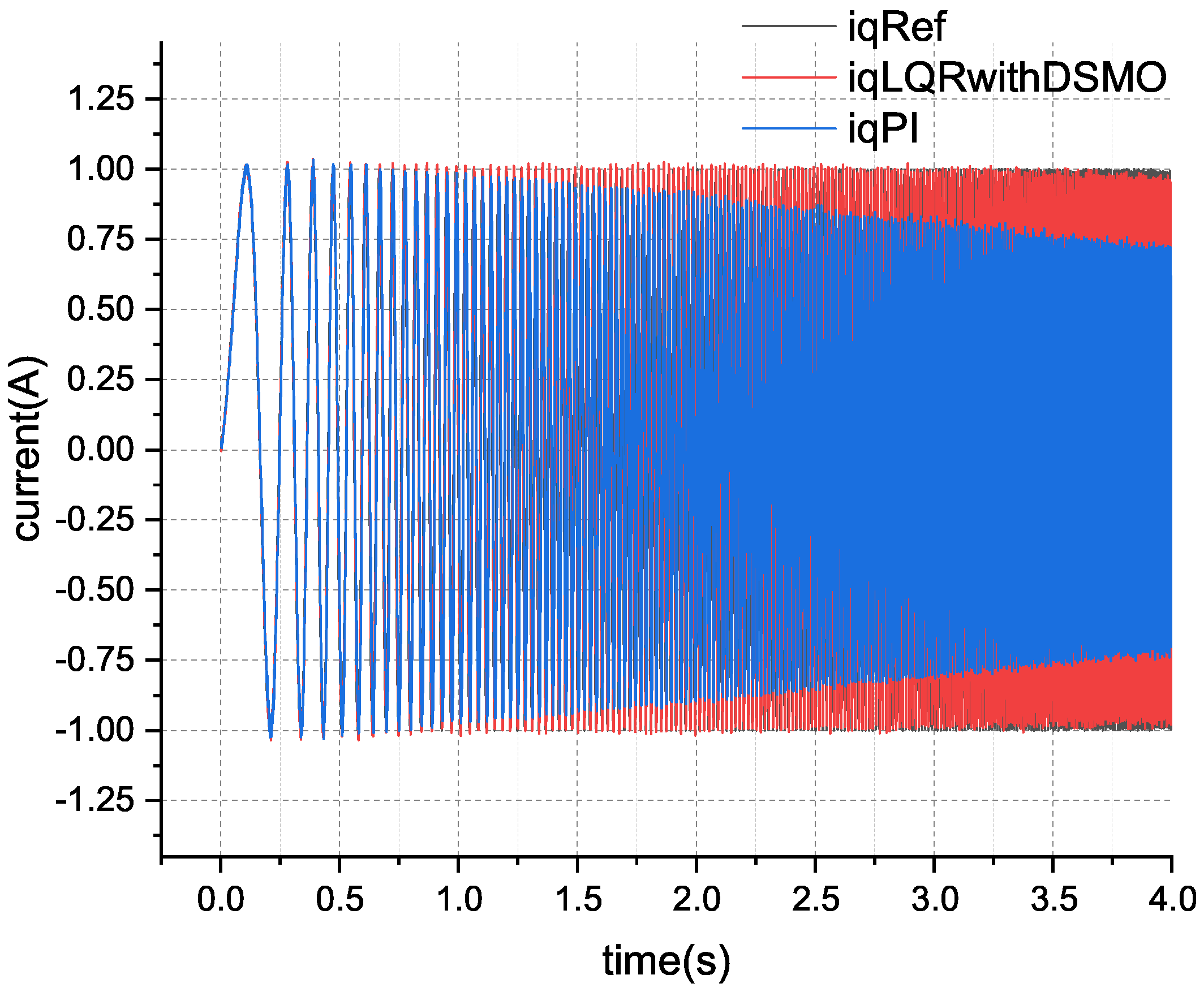
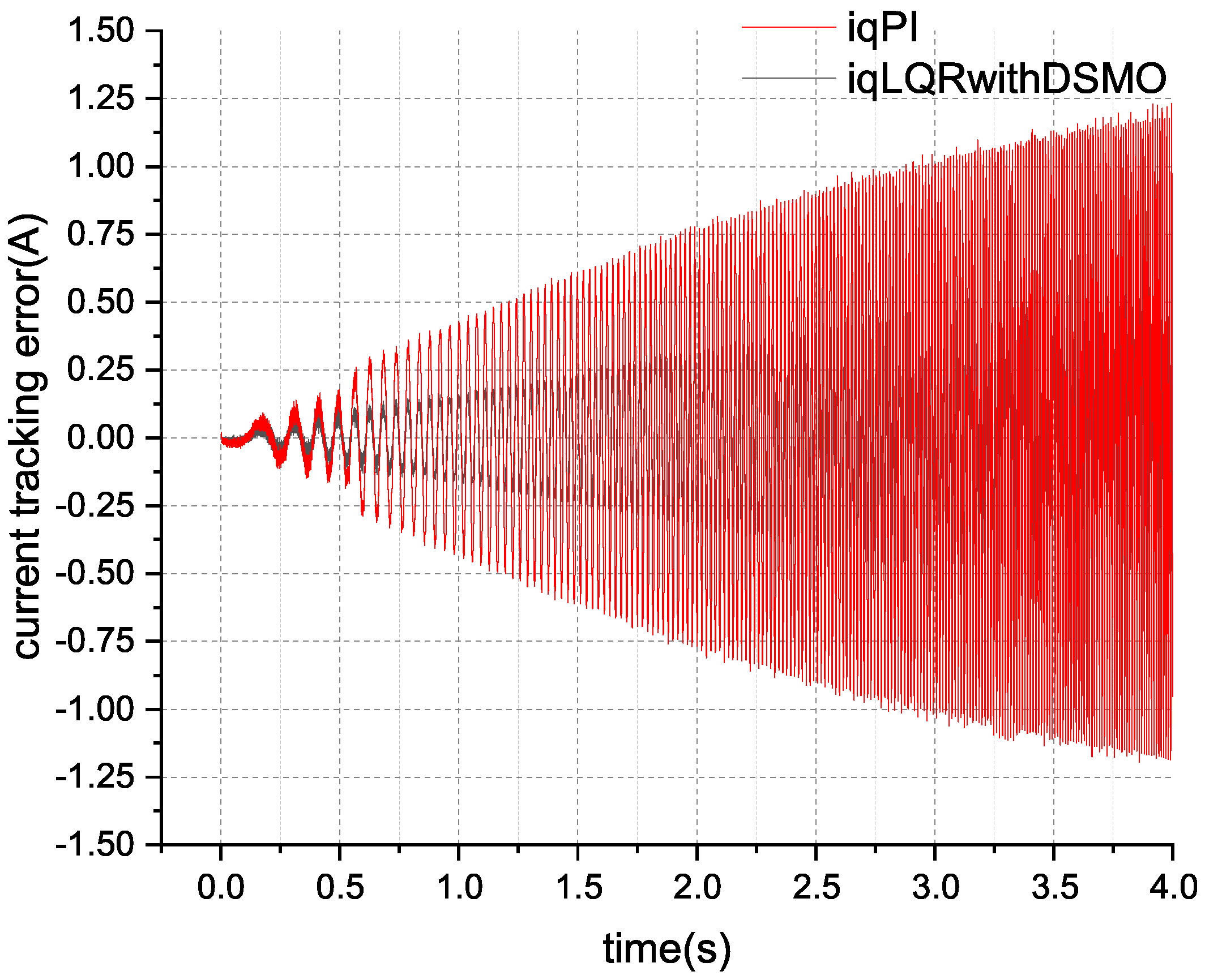
In order to further verify the performance of the designed control scheme, current loop sweep frequency experiments were conducted under simulation conditions compared with the classical PI controller. The reference value of the current loop adopts a chirp signal with an amplitude of 1.0 A, and the frequency rises from 100 Hz to 1000 Hz within 0.05 s. The result is shown in Figure 6.
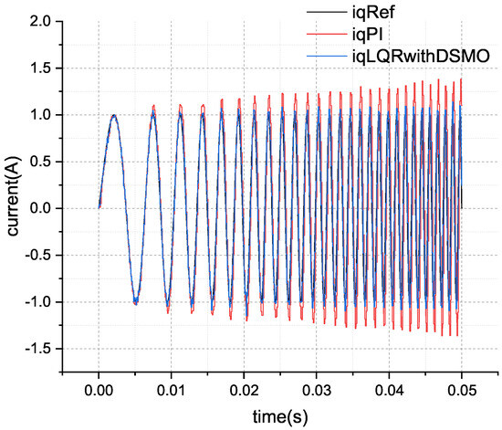
Figure 6.
Current tracking result when the frequency varies from 100 Hz to 1000 Hz.
The comparison results of the current tracking error are shown in Figure 7. From Figure 7, it can be seen that as the frequency of current changes increases, the tracking error of the classic PI controller significantly increases, with a current tracking RMSE of 0.4289. The current tracking RMSE of the control scheme proposed in this paper is 0.1569, which improves the performance by about 63.41%.
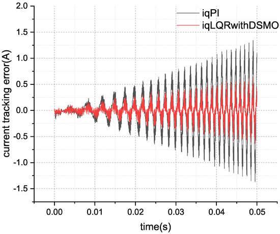
Figure 7.
Current tracking error result when the frequency varies from 100 Hz to 1000 Hz.
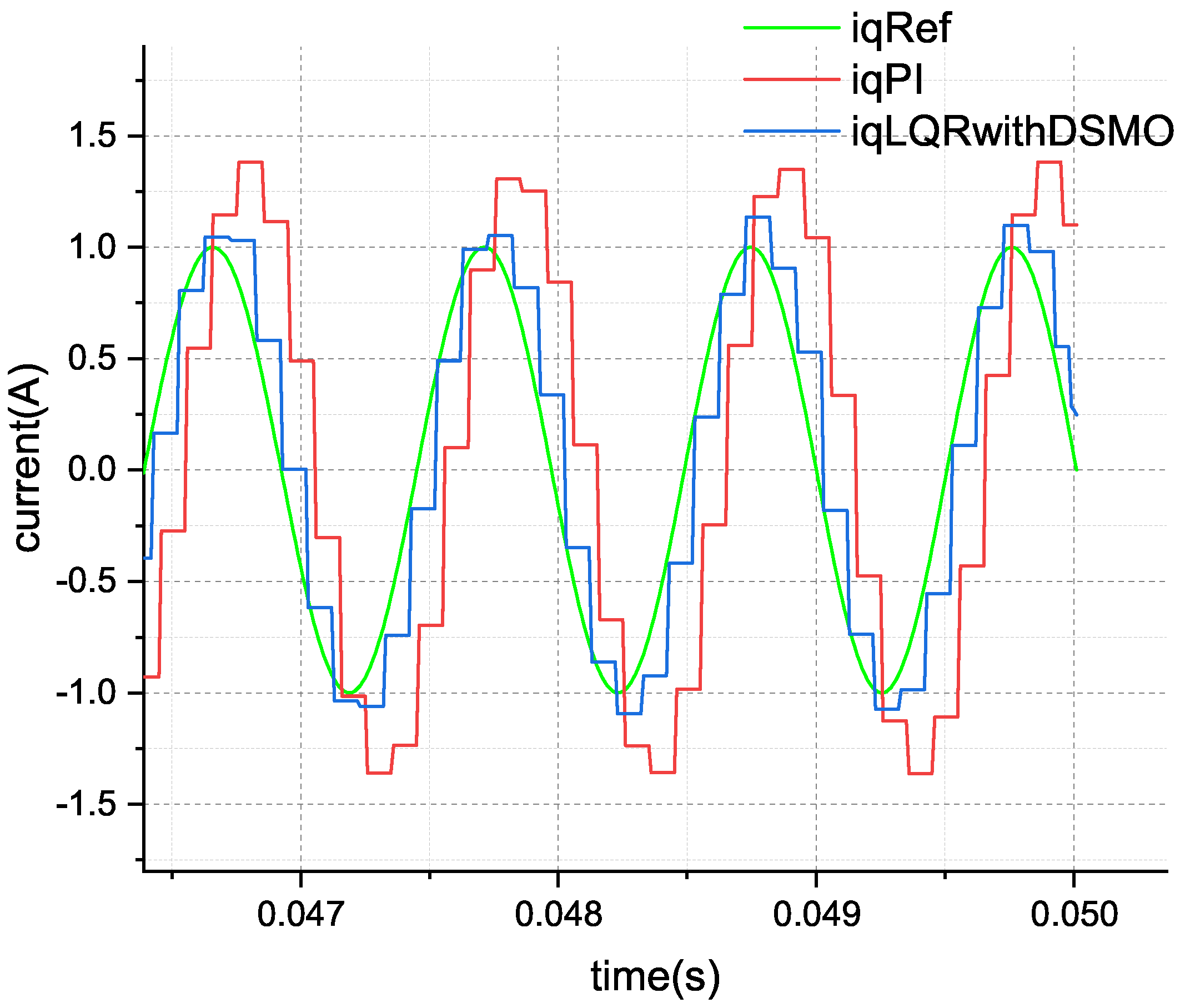
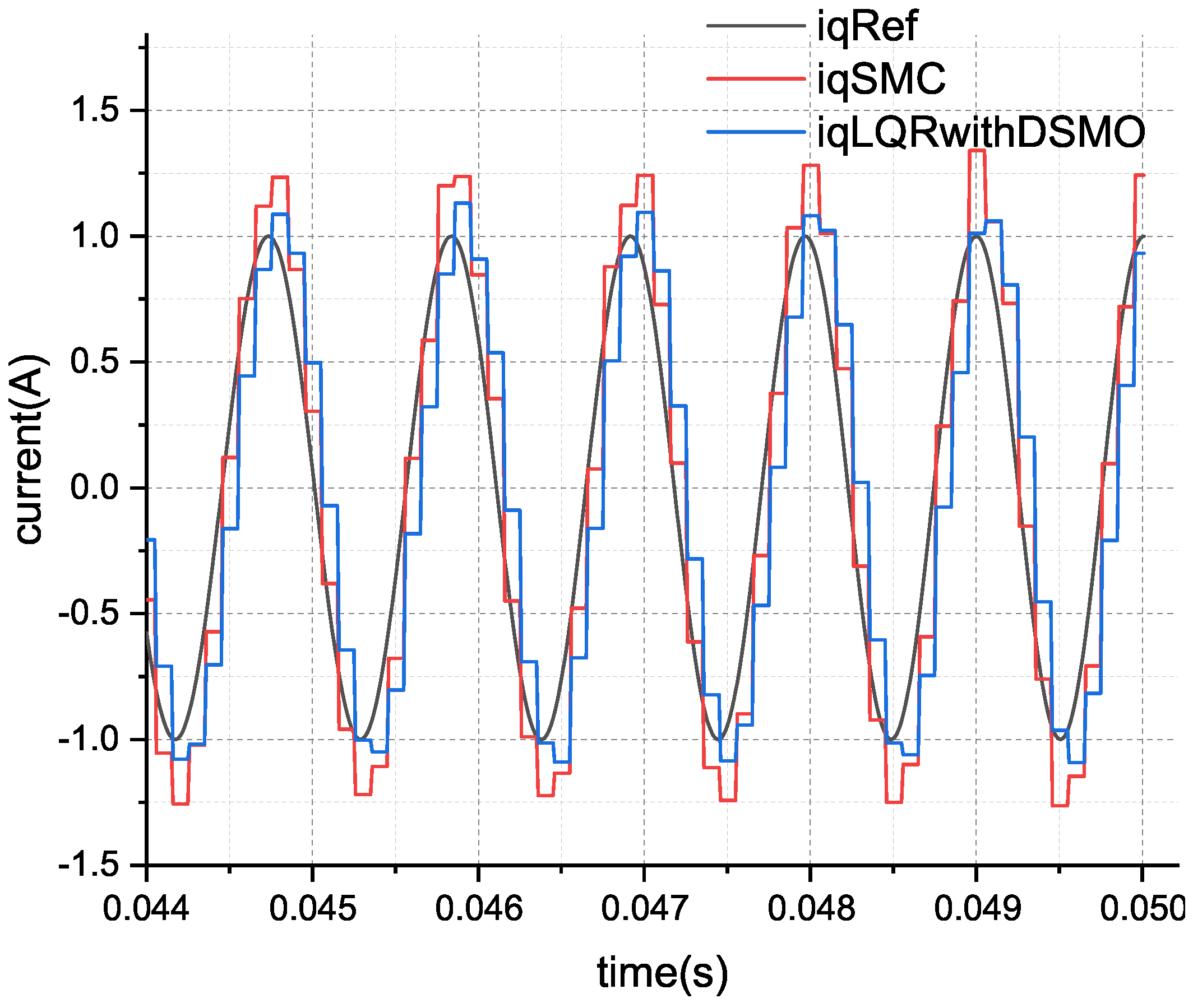
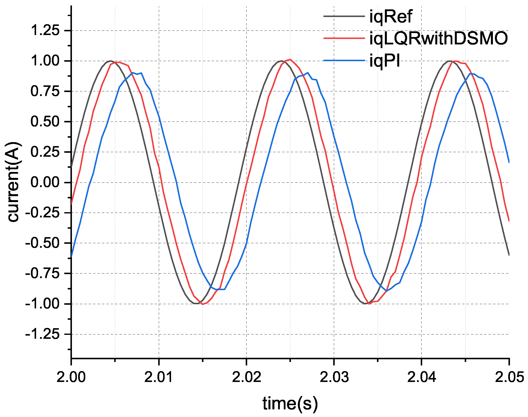
The current tracking variation near the frequency sweep signal of about 1000 Hz is shown in Figure 8.
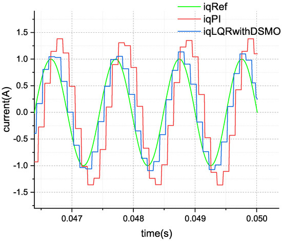
Figure 8.
Current tracking variation at frequency 1000 Hz.
In Figure 8, the green curve represents the reference value of the q-axis current, the blue curve represents the current tracking result of the control scheme proposed in this paper, and the red curve represents the current tracking result of the classical PI controller. In comparison, the classical PI controller shows a significant phase lag and tracking error.
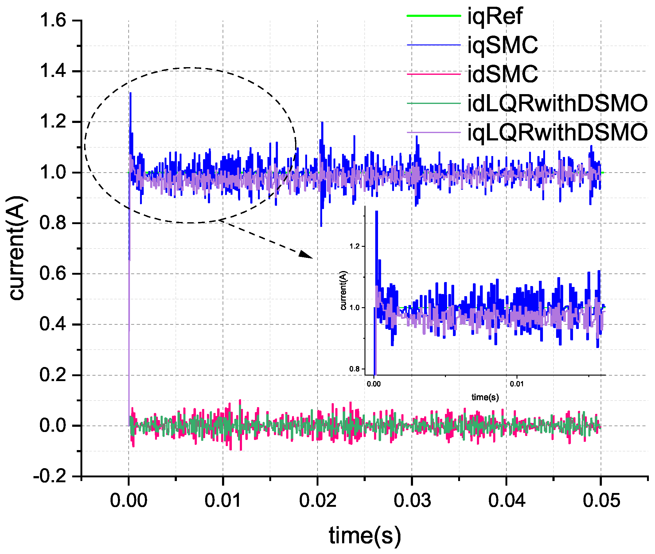
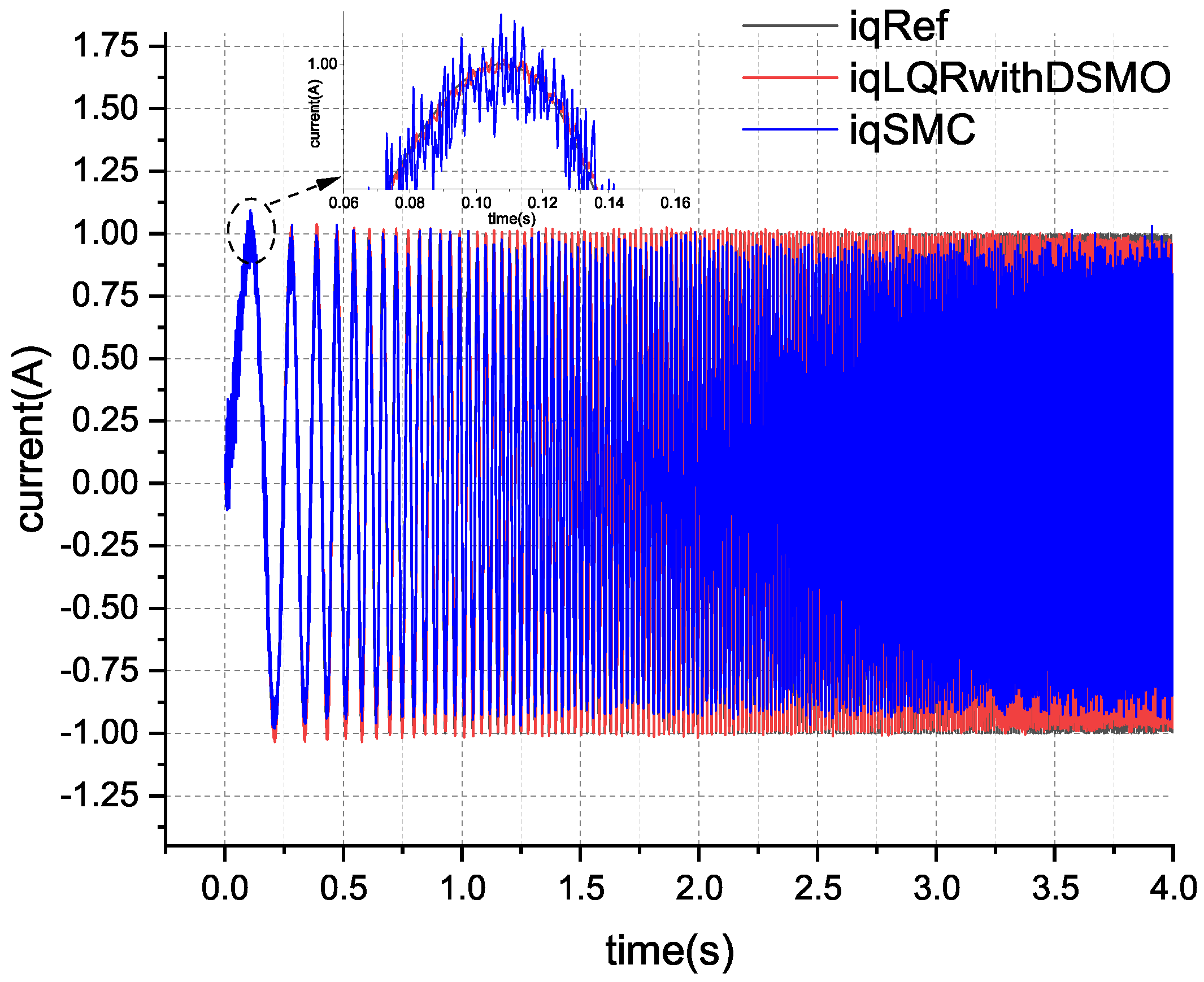
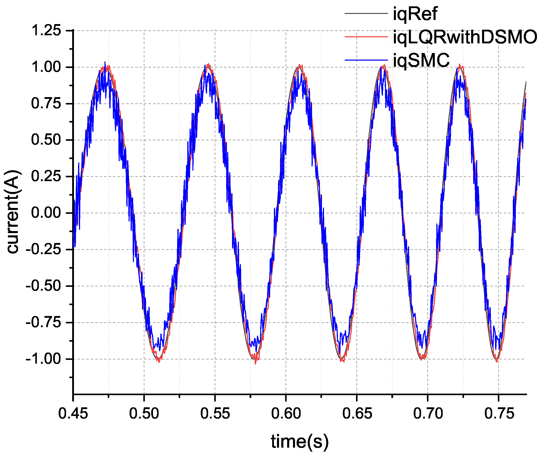
The primary objective of the disturbance observer proposed in this paper is to suppress disturbances within the control loop, which aligns with the goal of direct sliding mode control. To further validate the performance of the method introduced in this paper, a comparative analysis was conducted with an improved sliding mode control scheme. The improved sliding mode control strategy employs a saturation function in lieu of the signum function to mitigate the chattering phenomenon typically associated with traditional sliding mode control, which is a commonly adopted approach. The comparative results between the method proposed in this paper and the improved sliding mode control scheme, as demonstrated through computer simulations, are illustrated in Figure 9.

Figure 9.
Comparative results of current step tracking performance between the proposed method and the improved SMC scheme.
The step response current tracking RMSE for the proposed scheme, the improved sliding mode control scheme, and the classical PI control scheme are presented in Table 3.
Table 3.
The step response current tracking RMSE of different schemes.
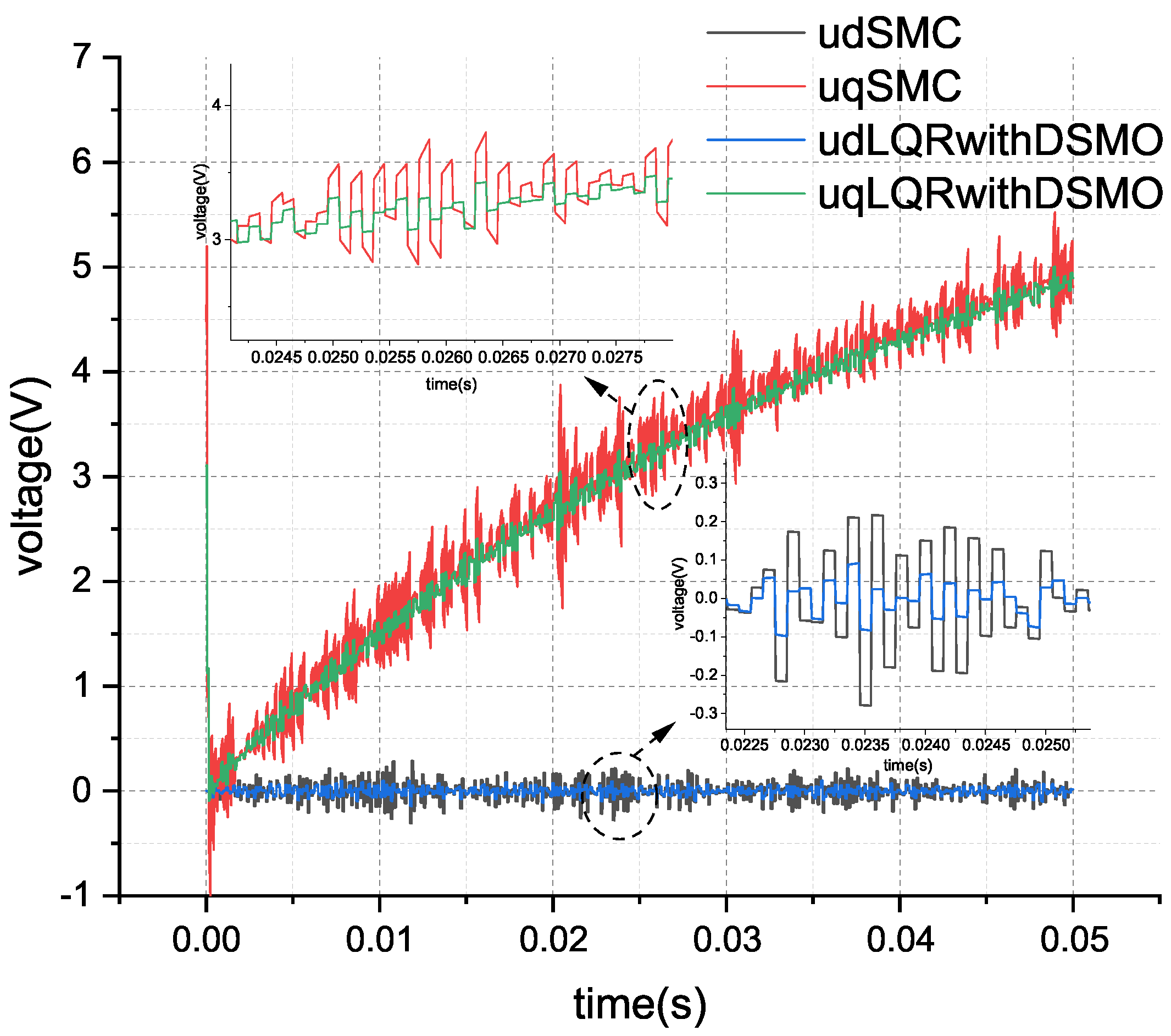
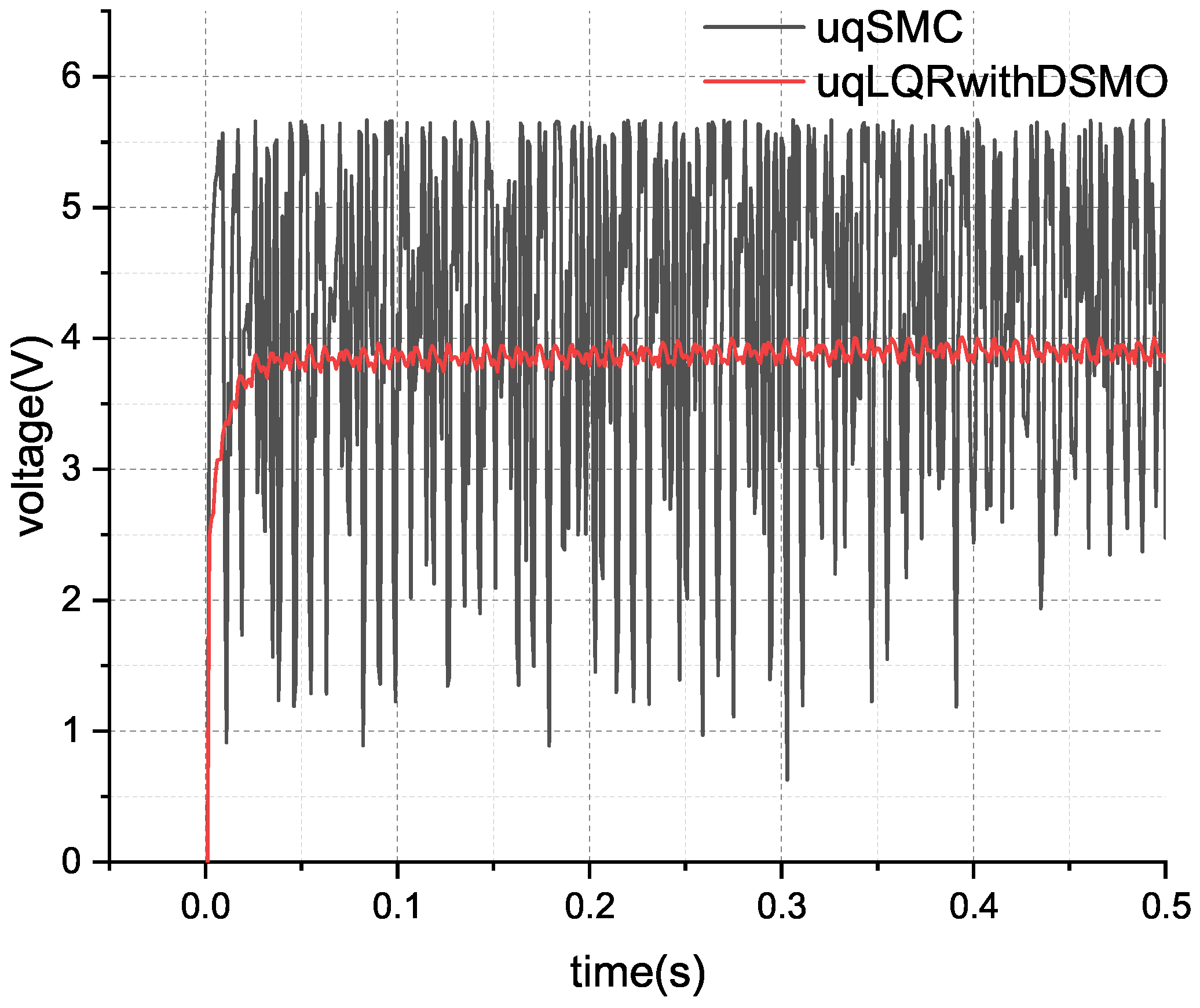
From the rise phase of the current in Figure 9, it can be observed that the current under sliding mode control can rapidly reach the reference current and fluctuate around it, indicating that sliding mode control possesses a strong disturbance rejection capability. However, the dynamic error of these fluctuations also becomes significantly larger. As shown in Table 3, the calculation results of the RMSE for current tracking demonstrate that the performance of the improved sliding mode control in tracking current is superior to that of the PI controller in terms of root mean square error, but it is not as effective as the method proposed in this paper. This is attributed to the fact that the disturbance rejection and rapid response of sliding mode control are achieved by swiftly changing the direction of the control effort, thereby forcing the system state to oscillate around the sliding surface. Consequently, despite modifications to the switching function in the sliding mode control, the inherent chattering phenomenon remains challenging to eliminate. The comparison of control efforts during the current tracking process is depicted in Figure 10.

Figure 10.
Comparative results of control effort between the proposed method and the improved SMC scheme.
The simulation results depicted in Figure 10 reveal that the red curve, labeled ’uqSMC’, represents the control effort of the improved sliding mode control for the q-axis voltage, while the green curve, marked ‘uqLQRwithDSMO’, corresponds to the control effort of the method proposed in this paper. It is evident that, in order to suppress disturbances, the sliding mode control exhibits a larger fluctuation in its control effort, which can induce vibrations throughout the system and potentially reduce the service life of the mechanical structure.
The sweep frequency simulation results for the current loop are illustrated in Figure 11 and Figure 12. The sweep frequency current tracking RMSE of the three control schemes is presented in Table 4.
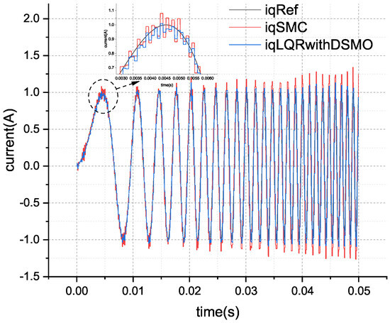
Figure 11.
Current tracking comparative result when the frequency varies from 100 Hz to 1000 Hz between the proposed method and the improved SMC scheme.
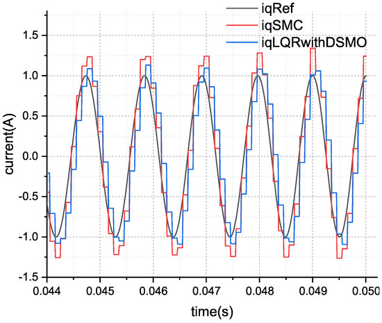
Figure 12.
Current tracking comparative result between the proposed method and the improved SMC scheme at frequency around 1000 Hz.
Table 4.
The sweep frequency response current tracking RMSE of different schemes.
From Figure 11 and Figure 12, it can be observed that the tracking current under sliding mode control fluctuates rapidly around the reference current, yet with considerable error, as indicated in Table 4, which is still indicative of chattering. It is evident that to achieve good disturbance rejection performance, even with improved sliding mode control, the inherent chattering phenomenon is difficult to eliminate. In contrast, the control method proposed in this paper does not have the aforementioned issues while resisting disturbance.
5.3. Experiment Protocol
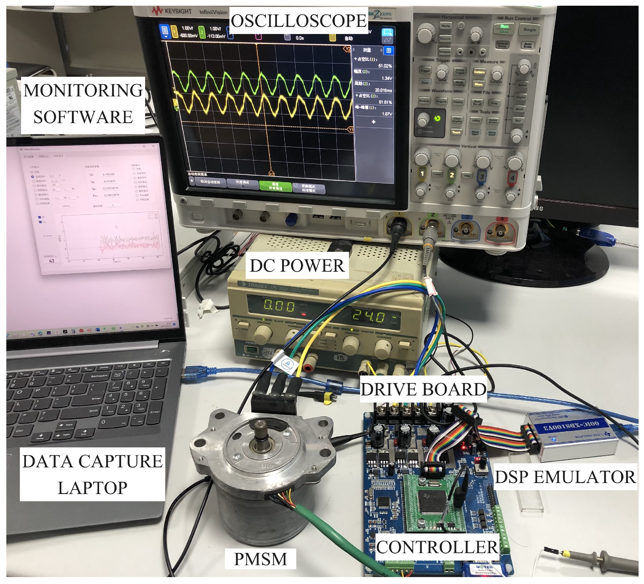
Validation experiments are conducted to compare the classical PI control method used widely in engineering with the current loop control scheme proposed in this paper. The hardware experimental environment used is shown in Figure 13.
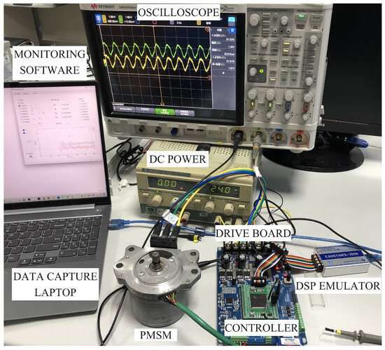
Figure 13.
Experimental setup.
The PMSM tested in the validation experiment is the MITSUBA-PA66-GF30, and the real-time controller 32-bit floating point DSP (TMS320F28335, manufactured by Texas Instruments in Dallas, TX, USA) is used, which can run at 150 MHz system frequency, in order to process the measurement information, the FOC control algorithm, the PI control law, the proposed disturbance observer, and the output SVPWM waveform driving power board.
Two current Hall sensors (ACS758LCB-050B, manufactured by Allegro MicroSystems in Manchester, NH, USA) are used to measure the phase current of the PMSM, which are converted into a digital signal through the 12 bit ADC of DSP. The current of the third phase is calculated using Kirchhoff’s current law for the conversion from a stator -axis to a -axis synchronous coordinate system. A resolver scheme is adopted to measure the shaft rotation by the angle signal acquisition chip (AD2S1205, manufactured by Analog Devices in Norwood, MA, USA), which can achieve 12-bit resolution digital conversion. Six metal oxide semiconductor field effect transistors (HY3610, manufactured by Hooyi Semiconductor, Xi’an, China) are used to construct the motor-driven circuit board in the form of three half-bridge circuits, achieving three-phase command voltage through an inverter supplied by DC 24 V power to drive the PMSM.
The nominal parameters of the PMSM used to validate the proposed observer scheme are given in Table 5.
Table 5.
The parameters of PMSM used in the validation experiment.
5.4. Experiment Results and Discussion
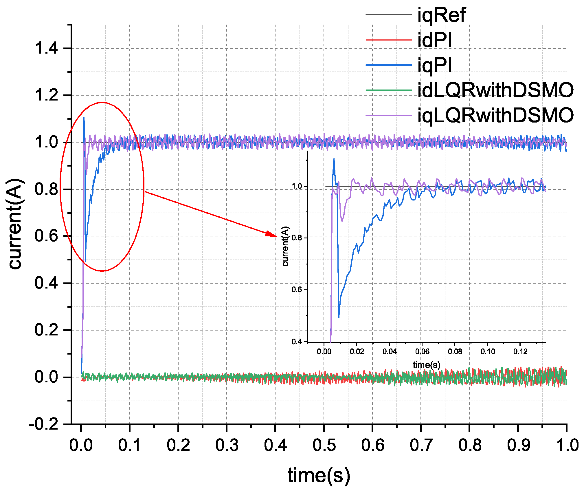
After setting the current loop q-axis command to 1.0 A and the d-axis command to 0.0 A, and starting the current loop control circuit, the comparison results obtained between the proposed control scheme and the classical PI controller current response are shown in Figure 14.
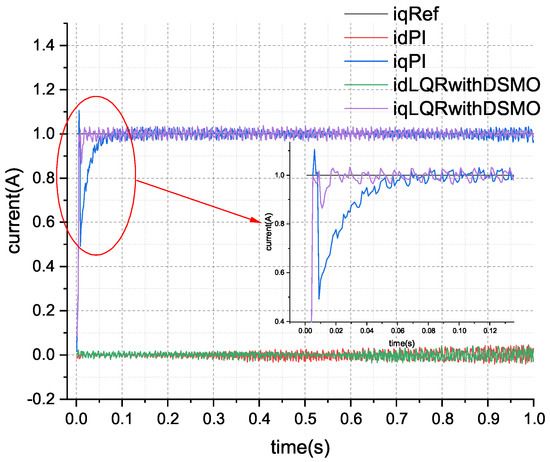
Figure 14.
Comparison diagram of step response control effects of the two schemes.
From the actual comparison results of current tracking, it can be seen that the current of the classic PI controller cannot stabilize at the reference value after rapidly rising above it. This is due to the internal disturbance generated by the circuit after operation, and the control error gradually decreases under the effect of integration. Compared to other methods, the LQR control scheme based on DSMO has a good anti-interference effect and can quickly and stably track the current reference value. The current tracking RMSE of classical PI control is 0.0716 A, while the current tracking RMSE of the LQR scheme based on DSMO is 0.0560 A, resulting in a 21.79% improvement in control performance.
The current state convergence results of DSMO are shown in Figure 15. From Figure 15, it can be seen that DSMO can quickly and accurately track the changes in actual current, indicating that the observer has achieved fast convergence. The estimation of disturbances in the -axis by the sliding mode observer is shown in Figure 16.
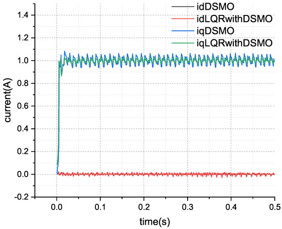
Figure 15.
Estimation and convergence experimental result of the sliding mode observer.
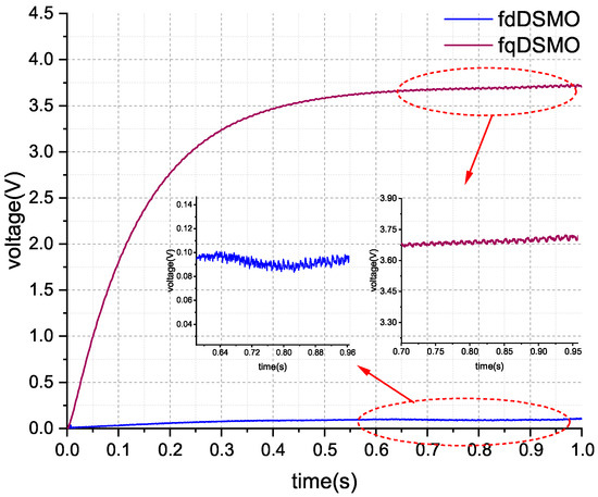
Figure 16.
Estimation result of the disturbance in the -axis in the experiment.
In order to fully verify the performance of the proposed control scheme, a sweep frequency test with an amplitude of 1.0 A and frequency change from 1.0 Hz to 101.0 Hz was conducted in actual PMSM current loop testing experiments, with a frequency increase time of 4.0 s. The results are shown in Figure 17.
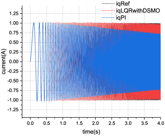
Figure 17.
Comparison result of linear sweep frequency experiment from 1.0 Hz to 101.0 Hz.
An enlarged diagram of the current tracking during the frequency sweep test is shown in Figure 18. A comparison of current tracking errors in the frequency sweep test of the two schemes is shown in Figure 19.
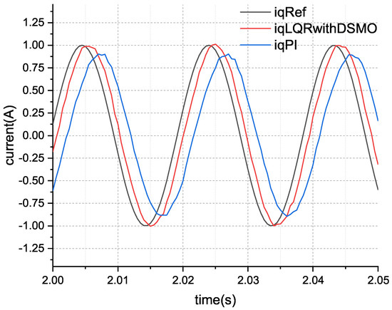
Figure 18.
Enlarged comparison results of linear sweep frequency experiment.
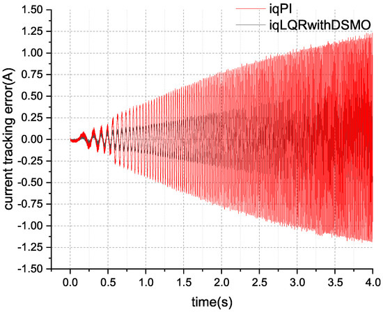
Figure 19.
Comparison tracking error result of linear sweep frequency experiment from 1.0 Hz to 101.0 Hz.
From the comparison results in Figure 17 and Figure 18 tests, it can be seen that classical PI control can track the current changes well in the low-frequency range. When the current changes quickly, the tracking effect of LQR control based on DSMO is significantly better than that of classical PI control. From the current amplification diagram during the frequency sweep process, it can be seen that for the current command curve (black curve, iqRef), there is a significant phase delay and tracking error in the classical PI control (blue curve, iqPI) compared to the DSMO-based LQR (red curve, iqLQRwithDSMO). After calculation, the current tracking RMSE of the classical PI control is 0.5621 A, while the current tracking RMSE of the proposed control scheme is 0.2582 A. Under the frequency sweep test conditions, the control accuracy was improved by about 54.07% using the scheme proposed in this paper.
The comparative experimental results between the method proposed in this paper and the improved SMC scheme are shown in Figure 20. The step response current tracking RMSE for the three control schemes is depicted in Table 6.
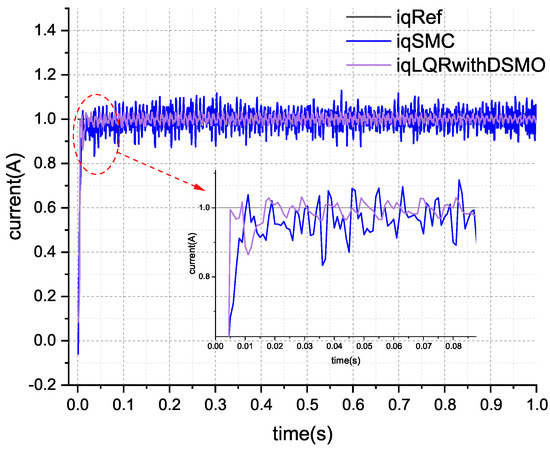
Figure 20.
The comparative experimental results of current step tracking performance between the proposed method and the improved SMC scheme.
Table 6.
Experimental step response current tracking RMSE of different schemes.
The hardware expriment results in Figure 20 indicate that the tracking current of the improved sliding mode control exhibits significant fluctuations around the reference value, and the chattering phenomenon is difficult to completely eliminate. The RMSE calculation results for current tracking in Table 6 show that the tracking performance of the improved sliding mode control is superior to that of the classical PI controller, but it is not as effective as the method proposed in this paper, which is in basic agreement with the simulation results and discussion conclusions. The actual control efforts during the experimental process are compared as shown in Figure 21.
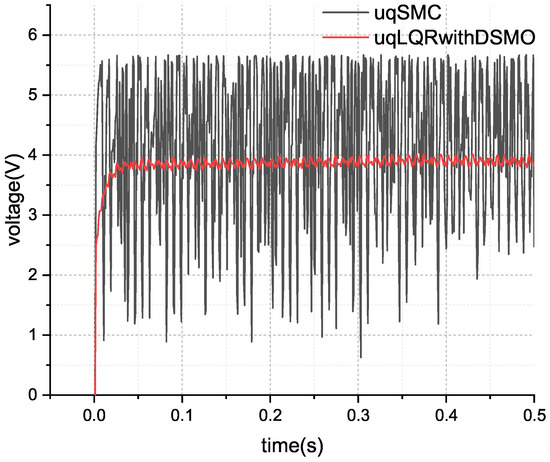
Figure 21.
Experimental comparative results of control effort between the proposed method and the improved SMC scheme.
The experimental validation results depicted in Figure 21 reveal that the black curve labeled ’uqSMC’ corresponds to the control effort of the q-axis voltage in the improved sliding mode control, while the red curve marked ‘uqLQRwithDSMO’ represents the actual control effort of the method proposed in this paper. It is evident that, in order to suppress disturbances, the control effort in sliding mode control fluctuates significantly, which may induce vibrations throughout the system and potentially reduce the service life of the mechanical structure. This finding is consistent with the conclusions drawn from the simulation analysis.
The comparative experimental results of the sweep frequency test for the current loop are illustrated in the subsequent Figure 22 and Figure 23. The RMSE of the sweep frequency experimental current tracking for the three control schemes is presented in Table 7.
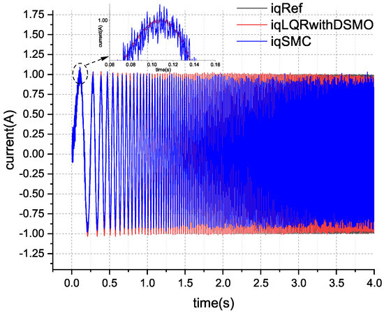
Figure 22.
Current tracking comparative experimental result when the frequency varies from 1.0 Hz to 101.0 Hz between the proposed method and the improved SMC scheme.

Figure 23.
Enlarged comparison results of linear sweep frequency experiment between the proposed method and the improved SMC scheme.
Table 7.
Sweep frequency experimental response current tracking RMSE of different schemes.
From Figure 22 and Figure 23, it is observed that the actual current under sliding mode control fluctuates rapidly around the reference current, albeit with a significant error, as demonstrated in Table 7, which is indicative of persistent chattering. To achieve robust disturbance rejection, the improved sliding mode control still struggles to eliminate its inherent chattering issues. In contrast, the control method proposed in this paper effectively resists disturbance without the chattering problem. The actual experimental validation results and analytical conclusions are fundamentally consistent with the simulation findings.
6. Conclusions
In this paper, a current loop control model with disturbance is first established, and subsequently an LQR controller based on a disturbance sliding mode observer is proposed to improve current tracking performance. There are inevitable disturbances in the -axis decoupling control loop of permanent magnet synchronous motors, resulting in current tracking errors within the controller. The integration effect in the classic PI controller widely used in engineering demonstrates a certain disturbance suppression capability. Because of the time required for integration, the disturbance suppression speed is obviously slow. Moreover, increasing the integration coefficient of the PI controller is not a good solution, as excessive integration coefficients can cause system instability. Furthermore, through comparative simulations and experimental results with the improved sliding mode control scheme, the disturbance suppression scheme based on the sliding mode observer proposed in this paper possesses the capability to resist disturbances without the encumbrance of chattering issues. In summary, the disturbance sliding mode observer proposed in this paper can achieve rapid real-time estimation and compensation of the disturbances in the control loop. Consequently, the linearized feedforward LQR controller by DSMO can improve the precision of current loop control.
In conclusion, this paper represents a straightforward and effective current control scheme suitable for servo-engineering applications of surface-mounted PMSMs.
Author Contributions
This paper was accomplished by all the authors. Z.Z., J.F. and T.L. proposed the idea, performed the analysis, and designed the simulation; Z.Z. and J.F. carried out the simulations and validation experiments; and Z.Z., J.F., G.Y. and Q.C. co-wrote the manuscript. All authors have read and agreed to the published version of the manuscript.
Funding
This work was supported by the National Natural Science Foundation of China (61803015).
Data Availability Statement
The data are not publicly available due to privacy.
Conflicts of Interest
Author Jing Fan was employed by the company China State Shipbuilding Corporation Limited. The remaining authors declare that the research was conducted in the absence of any commercial or financial relationships that could be construed as a potential conflict of interest.
Abbreviations
The following abbreviations are used in this manuscript:
| PMSM | Permanent magnet synchronous motor |
| DSMO | Disturbance sliding mode observer |
| SMO | Sliding mode observer |
| SMC | Sliding mode control |
| LQR | Linear quadratic regulator |
| SVPWM | Space vector pulse width modulation |
| FCS-M2PC | Finite control set modulation model predictive control |
| NN | Neural network |
| PI | Proportional integral |
| MPC | Model predictive control |
References
- Rafaq, M.S.; Jung, J.W. A Comprehensive Review of State-of-the-Art Parameter Estimation Techniques for Permanent Magnet Synchronous Motors in Wide Speed Range. IEEE Trans. Ind. Inform. 2020, 16, 4747–4758. [Google Scholar] [CrossRef]
- Inoue, T.; Inoue, Y.; Morimoto, S.; Sanada, M. Maximum Torque Per Ampere Control of a Direct Torque-Controlled PMSM in a Stator Flux Linkage Synchronous Frame. IEEE Trans. Ind. Appl. 2016, 52, 2360–2367. [Google Scholar] [CrossRef]
- Königseder, F.; Kemmetmüller, W.; Kugi, A. Attitude control strategy for a camera stabilization platform. Mechatronics 2017, 46, 60–69. [Google Scholar] [CrossRef]
- Liu, H.; Li, S. Speed Control for PMSM Servo System Using Predictive Functional Control and Extended State Observer. IEEE Trans. Ind. Electron. 2012, 59, 1171–1183. [Google Scholar] [CrossRef]
- Yin, Y.; Liu, L.; Vazquez, S.; Xu, R.; Dong, Z.; Liu, J.; Leon, J.I.; Wu, L.; Franquelo, L.G. Disturbance and Uncertainty Attenuation for Speed Regulation of PMSM Servo System Using Adaptive Optimal Control Strategy. IEEE Trans. Transp. Electrif. 2023, 9, 3410–3420. [Google Scholar] [CrossRef]
- Bu, F.; Yang, Z.; Gao, Y.; Pan, Z.; Pu, T.; Degano, M.; Gerada, C. Speed Ripple Reduction of Direct-Drive PMSM Servo System at Low-Speed Operation Using Virtual Cogging Torque Control Method. IEEE Trans. Ind. Electron. 2021, 68, 160–174. [Google Scholar] [CrossRef]
- Yuan, T.; Chang, J.; Zhang, Y. Parameter Identification of Permanent Magnet Synchronous Motor with Dynamic Forgetting Factor Based on H-infinite Filtering Algorithm. Actuators 2023, 12, 453. [Google Scholar] [CrossRef]
- Candelo-Zuluaga, C.; Riba, J.R.; Garcia, A. PMSM Parameter Estimation for Sensorless FOC Based on Differential Power Factor. IEEE Trans. Instrum. Meas. 2021, 70, 1–12. [Google Scholar] [CrossRef]
- Sandre-Hernandez, O.; Morales-Caporal, R.; Rangel-Magdaleno, J.; Peregrina-Barreto, H.; Hernandez-Perez, J.N. Parameter Identification of PMSMs Using Experimental Measurements and a PSO Algorithm. IEEE Trans. Instrum. Meas. 2015, 64, 2146–2154. [Google Scholar] [CrossRef]
- Wang, Q.; Wang, G.; Zhao, N.; Zhang, G.; Cui, Q.; Xu, D. An Impedance Model-Based Multiparameter Identification Method of PMSM for Both Offline and Online Conditions. IEEE Trans. Power Electron. 2021, 36, 727–738. [Google Scholar] [CrossRef]
- Wallscheid, O.; Bocker, J. Global Identification of a Low-Order Lumped-Parameter Thermal Network for Permanent Magnet Synchronous Motors. IEEE Trans. Energy Convers. 2016, 31, 354–365. [Google Scholar] [CrossRef]
- Pulvirenti, M.; Scarcella, G.; Scelba, G.; Testa, A.; Harbaugh, M.M. On-Line Stator Resistance and Permanent Magnet Flux Linkage Identification on Open-End Winding PMSM Drives. IEEE Trans. Ind. Appl. 2019, 55, 504–515. [Google Scholar] [CrossRef]
- Raja, R.; Sebastian, T.; Wang, M.; Chowdhury, M. Stator inductance estimation for permanent magnet motors using the PWM excitation. In Proceedings of the 2017 IEEE Energy Conversion Congress and Exposition (ECCE), Cincinnati, OH, USA, 1–5 October 2017; IEEE: Piscataway, NJ, USA, 2017. [Google Scholar] [CrossRef]
- Rafaq, M.S.; Mwasilu, F.; Kim, J.; Choi, H.H.; Jung, J.W. Online Parameter Identification for Model-Based Sensorless Control of Interior Permanent Magnet Synchronous Machine. IEEE Trans. Power Electron. 2017, 32, 4631–4643. [Google Scholar] [CrossRef]
- Li, X.; Kennel, R. General Formulation of Kalman-Filter-Based Online Parameter Identification Methods for VSI-Fed PMSM. IEEE Trans. Ind. Electron. 2021, 68, 2856–2864. [Google Scholar] [CrossRef]
- Xiao, X.; Chen, C.; Zhang, M. Dynamic Permanent Magnet Flux Estimation of Permanent Magnet Synchronous Machines. IEEE Trans. Appl. Supercond. 2010, 20, 1085–1088. [Google Scholar] [CrossRef]
- Li, T.; Liang, C.; Su, D. UKF-based Offline Estimation of PMSM Magnet Flux Linkage Considering Inverter Dead-time Voltage Error. In Proceedings of the 2022 IEEE Applied Power Electronics Conference and Exposition (APEC), Houston, TX, USA, 20–24 March 2022; IEEE: Piscataway, NJ, USA, 2022. [Google Scholar] [CrossRef]
- Yang, N.; Zhang, S.; Li, X.; Li, X. A New Model-Free Deadbeat Predictive Current Control for PMSM Using Parameter-Free Luenberger Disturbance Observer. IEEE J. Emerg. Sel. Top. Power Electron. 2023, 11, 407–417. [Google Scholar] [CrossRef]
- He, L.; Wang, F.; Wang, J.; Rodriguez, J. Zynq Implemented Luenberger Disturbance Observer Based Predictive Control Scheme for PMSM Drives. IEEE Trans. Power Electron. 2020, 35, 1770–1778. [Google Scholar] [CrossRef]
- Wang, W.; Liu, C.; Song, Z.; Dong, Z. Harmonic Current Suppression for Dual Three-Phase PMSM Based on Deadbeat Control and Disturbance Observer. IEEE Trans. Ind. Electron. 2023, 70, 3482–3492. [Google Scholar] [CrossRef]
- Zhao, Y.; Liu, X.; Yu, H.; Yu, J. Model-free adaptive discrete-time integral terminal sliding mode control for PMSM drive system with disturbance observer. IET Electr. Power Appl. 2020, 14, 1756–1765. [Google Scholar] [CrossRef]
- Yang, C.; Hua, T.; Dai, Y.; Huang, X.; Zhang, D. Second-Order Nonlinear Disturbance Observer Based Adaptive Disturbance Rejection Control for PMSM in Electric Vehicles. J. Electr. Eng. Technol. 2022, 18, 1919–1930. [Google Scholar] [CrossRef]
- Ahn, H.; Kim, S.; Park, J.; Chung, Y.; Hu, M.; You, K. Adaptive Quick Sliding Mode Reaching Law and Disturbance Observer for Robust PMSM Control Systems. Actuators 2024, 13, 136. [Google Scholar] [CrossRef]
- Turker, T.; Buyukkeles, U.; Bakan, A.F. A Robust Predictive Current Controller for PMSM Drives. IEEE Trans. Ind. Electron. 2016, 63, 3906–3914. [Google Scholar] [CrossRef]
- Li, Y.; Li, Y.; Wang, Q. Robust Predictive Current Control With Parallel Compensation Terms Against Multi-Parameter Mismatches for PMSMs. IEEE Trans. Energy Convers. 2020, 35, 2222–2230. [Google Scholar] [CrossRef]
- Mohamed, Y.R. Design and Implementation of a Robust Current-Control Scheme for a PMSM Vector Drive With a Simple Adaptive Disturbance Observer. IEEE Trans. Ind. Electron. 2007, 54, 1981–1988. [Google Scholar] [CrossRef]
- Tan, L.N.; Cong, T.P.; Cong, D.P. Neural Network Observers and Sensorless Robust Optimal Control for Partially Unknown PMSM With Disturbances and Saturating Voltages. IEEE Trans. Power Electron. 2021, 36, 12045–12056. [Google Scholar] [CrossRef]
- Li, S.; Won, H.; Fu, X.; Fairbank, M.; Wunsch, D.C.; Alonso, E. Neural-Network Vector Controller for Permanent-Magnet Synchronous Motor Drives: Simulated and Hardware-Validated Results. IEEE Trans. Cybern. 2020, 50, 3218–3230. [Google Scholar] [CrossRef]
- Meng, Q.; Bao, G. A Novel Low-Complexity Cascaded Model Predictive Control Method for PMSM. Actuators 2023, 12, 349. [Google Scholar] [CrossRef]
- Grzesiak, L.M.; Tarczewski, T. Permanent magnet synchronous motor discrete linear quadratic speed controller. In Proceedings of the 2011 IEEE International Symposium on Industrial Electronics, Gdansk, Poland, 27–30 June 2011; IEEE: Piscataway, NJ, USA, 2011. [Google Scholar] [CrossRef]
- Suleimenov, K.; Do, T.D. Data-Driven LQR for Permanent Magnet Synchronous Machines. In Proceedings of the 2019 IEEE Vehicle Power and Propulsion Conference (VPPC), Hanoi, Vietnam, 14–17 October 2019; IEEE: Piscataway, NJ, USA, 2019. [Google Scholar] [CrossRef]
- Mora, A.; Orellana, A.; Juliet, J.; Cardenas, R. Model Predictive Torque Control for Torque Ripple Compensation in Variable-Speed PMSMs. IEEE Trans. Ind. Electron. 2016, 63, 4584–4592. [Google Scholar] [CrossRef]
- Yu, F.; Li, K.; Zhu, Z.; Liu, X. An Over-Modulated Model Predictive Current Control for Permanent Magnet Synchronous Motors. IEEE Access 2022, 10, 40391–40401. [Google Scholar] [CrossRef]
- Sun, X.; Wu, M.; Lei, G.; Guo, Y.; Zhu, J. An Improved Model Predictive Current Control for PMSM Drives Based on Current Track Circle. IEEE Trans. Ind. Electron. 2021, 68, 3782–3793. [Google Scholar] [CrossRef]
- Zhang, X.; Cao, Y.; Zhang, C.; Niu, S. Model Predictive Control for PMSM Based on the Elimination of Current Prediction Errors. IEEE J. Emerg. Sel. Top. Power Electron. 2024, 12, 2651–2660. [Google Scholar] [CrossRef]


Disclaimer/Publisher’s Note: The statements, opinions and data contained in all publications are solely those of the individual author(s) and contributor(s) and not of MDPI and/or the editor(s). MDPI and/or the editor(s) disclaim responsibility for any injury to people or property resulting from any ideas, methods, instructions or products referred to in the content. |
© 2024 by the authors. Licensee MDPI, Basel, Switzerland. This article is an open access article distributed under the terms and conditions of the Creative Commons Attribution (CC BY) license (https://creativecommons.org/licenses/by/4.0/).