Article

Active Composite Control of Disturbance Compensation for Vibration Isolation System with Uncertainty

1
College of Intelligence Science and Technology, National University of Defense Technology, Changsha 410073, China
2
National Key Laboratory of Equipment State Sensing and Smart Support, Changsha 410073, China
*
Author to whom correspondence should be addressed.
Actuators 2024, 13(9), 334; https://doi.org/10.3390/act13090334
Submission received: 1 July 2024 / Revised: 25 August 2024 / Accepted: 26 August 2024 / Published: 3 September 2024
(This article belongs to the Special Issue New Control Schemes for Actuators—2nd Edition)

Abstract

:
The pointing and positioning accuracy of precision instruments in aerospace are often disturbed by low-frequency vibrations. An active/passive vibration isolation system is a feasible solution to suppress low-frequency vibrations. However, the vibration isolation performance of the active control strategy is seriously affected by the uncertainty of the system and the difficulty to meet the higher requirements of new-generation equipment. This paper proposes an active composite control (ACC) strategy for vibration isolation systems with uncertainty. The proposed ACC integrates feedforward control based on known systems and feedback control based on the Kalman filter for systems with uncertainty. Further, the derivation and stability analyses of the proposed ACC algorithm are provided, and the influence of system uncertainty on vibration isolation performance based on the proposed ACC is analyzed. Experimental verification is conducted and the experimental results confirm that the proposed ACC can effectively realize the low-frequency and wide-band vibration isolation for the system with uncertainty. Starting from 30 Hz, the vibration isolation performance of the proposed ACC with uncertainty is significantly improved than that of the ACC completely based on a deterministic system model.

1. Introduction

Mechanical vibration widely exists in aerospace equipment, which leads to serious interference in the pointing and positioning accuracy of precision instruments. In order to ensure the normal operation of precision instruments, it is necessary to take vibration isolation measures. Passive vibration isolation technology has been researched earlier and has been widely used. The typical standards include metal spring isolators [1], rubber isolators [2], wire rope isolators [3], and so on. However, these isolators generally have poor low-frequency vibration isolation performance and poor adaptability to the environment. Some scholars have proposed to apply the concept of quasi-zero stiffness to vibration isolation technology to broaden the bandwidth of vibration isolation [4,5,6,7]. However, in engineering applications, quasi-zero stiffness vibration isolators need to strictly ensure that the static position is in the design balance point. Once deviated from the design balance point, it may cause system instability or failure. Therefore, the tolerance for complex working conditions, processing errors, and installation errors is low, and it is still in the exploration stage.
The hybrid isolation that combines passive and active methods was introduced to make up for the deficiency of passive vibration isolation technology [8,9]. Active vibration isolation technology can regulate the system characteristics through an active control strategy and provides an effective way to realize low-frequency vibration isolation. At present, active control strategy, as one of the core parts of active vibration isolation technology, has become a research hotspot. The active control strategy can be divided into feedback control and feedforward control structurally [10,11,12,13]. The feedforward control strategy is a predictive control based on the controlled object model. If the feedforward control model is established accurately enough, the vibration of the base can be directly compensated by the controlling force, and the vibration isolation of the full frequency band can be realized [14,15]. However, there are many uncertainties in the practice system, such as parameter change, unknown disturbance, nonlinearity, and so on. The feedforward control makes it difficult to achieve the desired vibration isolation effect in applications. The feedback control strategy is to take the difference between the desired output and the current output of the controlled object as the input of the controller, and then affect the state of the controlled object to approach or achieve the desired output [16,17]. However, the performance of the feedback control is limited by issues, such as time delay and noise amplification. Moreover, high bandwidth vibration isolation through feedback control strategies can lead to stability problems [10]. Therefore, researchers use a combination of feedforward control and feedback control to improve vibration isolation performance, which can effectively compensate for the shortcomings of each other [9,18,19,20].
The logic processing of the control strategy depends on the control algorithm, and selecting a reasonable control algorithm is the key to ensuring vibration isolation performance. The classical PID control is more common in engineering, which has the advantages of an independent model and high reliability [21,22,23]. But, PID control is mainly suitable for linear time-invariant systems, and it is difficult to obtain the optimal control effect. In a system with a completely accurate model, state feedback control can theoretically provide both desired and achievable control effects. The optimal state feedback controller of the system can be designed by using the Luenberger observer and linear quadratic regulation (LQR) algorithm. Considering the uncertainty of the system model, the system robustness performance index is taken as the constraint design control law and transformed into a robust control problem [16,24]. Beijen et al. [25] carried out the parameter normalization analysis of the hybrid feedforward feedback control problem from the perspective of the H∞ performance constraints of the system, and designed the corresponding control law by solving two Riccati equations. Zhao et al. [26] designed a robust controller of H∞ based on the vibration isolation performance and the output range of the actuators, and the simulation results showed that the closed-loop transmissibility of the isolator was less than −18 dB in the frequency range from 0 to 100 Hz. However, the robust control system is usually designed based on the worst case, so the optimal control effect cannot be obtained. Adaptive control can better adapt to changes in the system and environment, and adjust control parameters in real time to ensure control effects [27]. Some researchers have carried out a series of adaptive control studies on different vibration isolation systems [28,29,30,31,32,33,34]. Landau et al. [35] combined the internal model principle with adaptive control to realize time-varying narrow-band disturbance rejection. Airimitoaie et al. [36] took advantage of the Youla/Kučera parametrization to solve the instability problem caused by a strong coupling between adaptive feedback and adaptive feedforward. Wang et al. [37] designed an adaptive sliding mode control algorithm to make an adaptive approximation of a vibration isolation system model with unknown dynamic parameters to a desired reference model. Davis et al. [38] designed an efficient and autonomous feedforward neural network control strategy, which adaptively compensates for unknown disturbance by adjusting its own weight online, so as to realize the adaptive cancelation of broadband vibration. But adaptive control also has disadvantages such as a slow convergence rate and poor stability.
To sum up, for the uncertainty problem of the system, the control algorithms commonly used at present (robust control, adaptive control, and so on) mainly have problems such as high control cost, too conservative, or poor stability. Therefore, some researchers made efforts to reduce or eliminate the influence of uncertainty on the system by compensating for the uncertainty of the system, and then combining the appropriate control algorithm to achieve the desired control effect. Various observers are proposed to estimate the uncertainty of the system, such as disturbance observer [39,40,41], extended state observer [42,43,44], etc. Zhang et al. [45] combined the disturbance observer with the active suspension saturation tracking control scheme based on switching logic to realize the evaluation of meaningful disturbance, which can be used for active suspension system control to reduce energy consumption. Ai et al. [46] combined extended state observer and LQR optimization algorithm in the output power control scheme of a hydraulic wind turbine and achieved higher control precision and stronger anti-interference. However, these disturbance observers are very sensitive to noise and often show a trade-off between noise amplification and disturbance estimation accuracy, which affects the final control effect.
Unlike the above observers, the Kalman filter [47] does not observe perturbations, but accurately estimates the current state of the system and eliminates the influence of measurement noise by data fusion between the predicted system output and the measured output. The Kalman filter has been successfully applied to many practical problems because of its excellent state estimation ability for uncertain systems. For instance, Bandopadhya et al. [48] used the Kalman filter to accurately estimate the tip deflection and tip deflection rate of the rotating flexible link and effectively suppressed the high-amplitude vibration of the flexible link by combining the active control scheme. Papadimitriou et al. [49] used the Kalman filter to predict the strain/stress response at various locations within structural components based on the measurements available at a limited number of locations, and further predict the expected fatigue damage accumulation. Based on the residual estimation of the Kalman filter, Erazo et al. [50] proposed a statistical method to decouple structural damage and temperature variations for damage assessment. Therefore, it is appropriate to use the Kalman filter to accurately estimate the state vector of uncertain systems for feedback control.
It is well known that uncertainties inevitably exist in practical vibration isolation systems. Nevertheless, part of the system information and disturbance can be accurately obtained by means of theory or experiments. In view of such characteristics, this paper employs an active composite control (ACC) strategy to improve the vibration isolation performance of the system. Based on the known disturbance and known system model information, the feedforward controller is designed to achieve two goals: on the one hand, the low frequency and broadband vibration isolation of the system is realized; on the other hand, the system stability is increased by reducing the burden of the feedback controller. The feedback control is a combination of the Kalman filter and the LQR algorithm (based on an internal model considering uncertainty). The Kalman filter is used to deal with the uncertainty of the system to obtain accurate system state variables (load displacement and load velocity), and then the LQR algorithm is used to optimize the state feedback gains. Thus, good vibration isolation performance can be achieved for the uncertain system with lower control cost and better stability compared with the existing methods.
This paper is organized as follows. In Section 2, a single-degree-of-freedom (SDOF) system is used as an object to verify the proposed ACC algorithm. Firstly, the SDOF system with uncertainty is modeled, and then according to the characteristics of the system, the ACC algorithm of this paper is proposed and described in detail. The derivation of the ACC algorithm and stability analysis, which consists of a feedforward control algorithm and a feedback control algorithm based on the Kalman filter, are provided in Section 3. Section 4 is the simulation analysis of the vibration isolation performance of the system with uncertainty. It mainly includes the influence of system uncertainty on feedforward control, the analysis of Kalman filter state estimation error, and the discussion of the active vibration isolation performance of the proposed ACC. In Section 5, to verify the feasibility of the proposed ACC algorithm, an SDOF vibration isolation experiment is carried out and compared with the results of the completely model-based ACC. The conclusion is summarized in Section 6.

2. System Description and Control Strategy

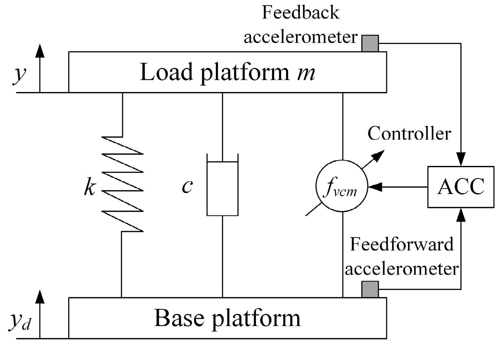
2.1. Problem Formulation

In practical engineering, there are many uncertainties in many vibration isolation systems, but part of the model information and part of the disturbance can be obtained. In this case, the purpose of this paper is to integrate the known model information, measurable disturbance, and other uncertainties into the controller design to improve the efficiency of active vibration isolation.

2.2. System Dynamics Modeling with Uncertainty

In order to better design the controller and ensure the accuracy of the control algorithm, it is necessary to establish a dynamic model. The object of this paper is a single-degree-of-freedom (SDOF) vibration isolation system as shown in Figure 1. The kinetic equation of the ideal vibration isolation system is as follows:
m y ¨ = k ( y y d ) c ( y ˙ y ˙ d ) + f v c m ,
where c and k are the system damping and stiffness, respectively. The variable y is the displacement of the mass m and yd is the displacement of the base. fvcm is the control force of the voice coil motor. Considering the existence of various disturbances in the system, Equation (1) can be rewritten as follows:
m y ¨ = c y ˙ k y Identification   system + f v c m Evaluated   force + c y ˙ d + k y d Measurable   disturbance + w Uncertainty ,
where the mass m is known. The damping c and stiffness k can be obtained by system identification. The control force fvcm is evaluated by motor thrust constant and control current. The base disturbance  c y ˙ d + k y d  can be measurable. The uncertainty w represents the influence of uncertain factors, including changing system parameters, unpredictable perturbations, fluctuating output forces, etc.
In the field of vibration control, accelerometers are often used to measure vibration signals, so the system state space equation takes the acceleration of the mass as output. Introducing the state vector  x = [ x 1 , x 2 ] T = [ y , y ˙ ] T , the form of the state space of Equation (2) can be expressed as follows:
x ˙ = A x + B u , z = C x + D u ,
where  A = 0 1 k m c m , B = 0 0 1 1 , C = k m c m , D = 1 1 , u = f v c m c y ˙ d + k y d + w .

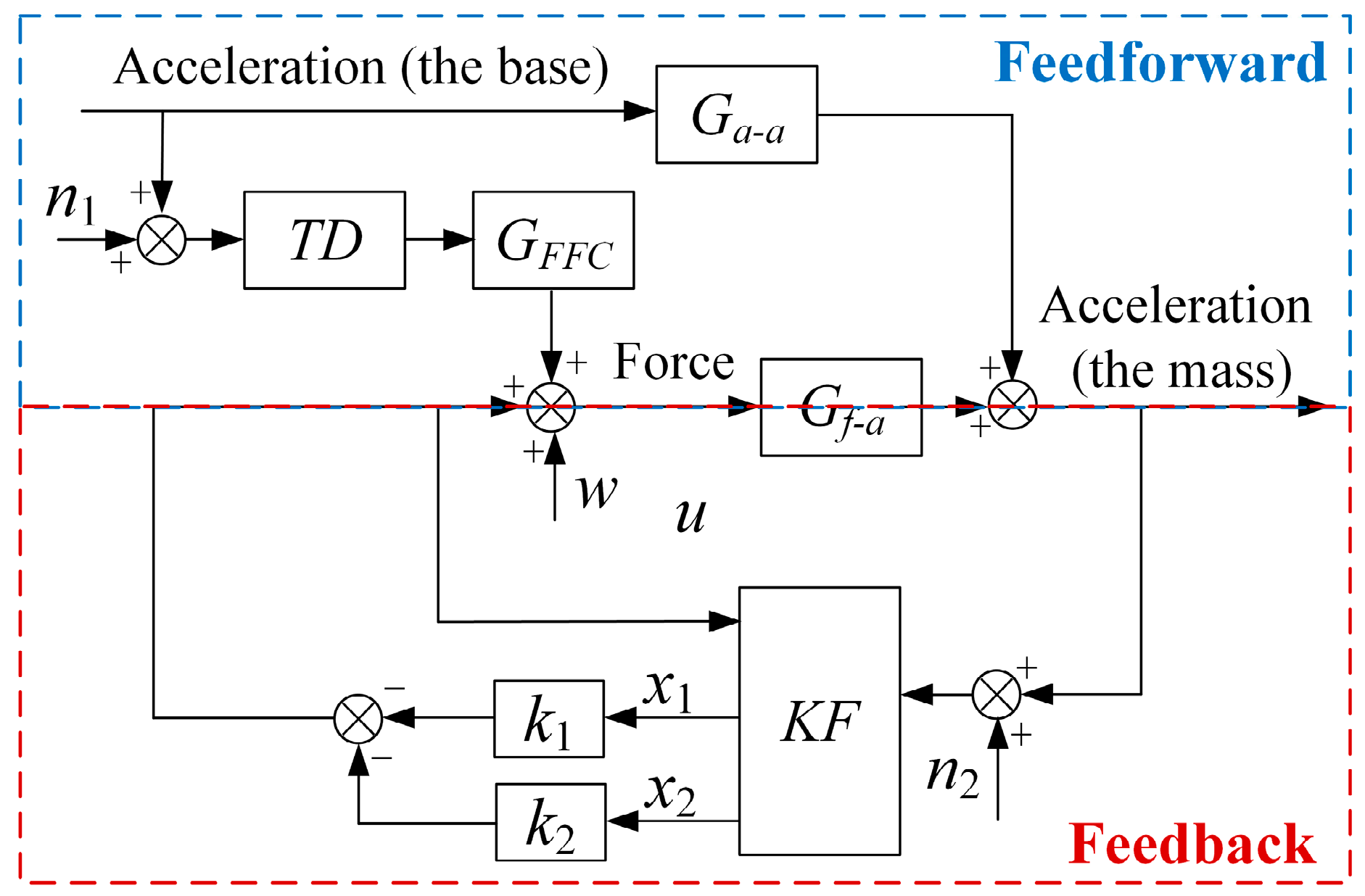
2.3. Composite Control Strategy

The SDOF hybrid control schematic is shown in Figure 1. A combination of feedforward and feedback control is adopted to suppress both base vibrations and some uncertain disturbances. The feedforward control loop is used to eliminate the base vibration, which can effectively improve vibration isolation bandwidth, and greatly reduce the burden of the feedback control loop. However, since there are some uncertainties in the system model, and some internal disturbances cannot be measured, the feedforward control cannot eliminate all the effects of disturbances. Therefore, the feedback control loop is necessary to further suppress the residual vibration after feedforward control and compensate for the disturbance of the unmeasured interference signal.
According to Figure 1, the hybrid controller structure is designed and presented in Figure 2. Ga-a represents the transfer function of the acceleration of the base to the acceleration of the mass, and Gf-a represents the transfer function of force on the mass to the acceleration of the mass. Based on the model information (Equation (2)), the feedforward controller GFFC is designed. Considering that the signal measured by the acceleration sensor has noise (n1), the tracking differentiator (TD) is used to filter the noise in the feedforward control loop. In the feedback control loop, the Kalman filter (KF) is adopted to estimate the state values (x1, x2) of the system with uncertainty (w) and noise (n2). The feedback controller is designed with the obtained state values (x1, x2), and the corresponding gains k1 and k2 are optimized by the LQR algorithm in this paper.

3. Composite Controller Design

3.1. Feedforward Control Loop

Since accelerometers are commonly used in vibration measurement and control applications, the transfer function mapping acceleration of the base to that of the mass according to Equation (2) can be expressed as follows:
G a a = s 2 Y ( s ) s 2 Y d ( s ) = c s + k m s 2 + c s + k .
The transfer function of force on the load mass to the acceleration of the load mass can be expressed as follows:
G f a = s 2 Y ( s ) F ( s ) = s 2 m s 2 + c s + k .
Therefore, the design of the ideal feedforward controller should meet the following condition:
G a a = G F F C G f a .
According to Equations (4)–(6), the form of the ideal feedforward controller can be expressed as follows:
G F F C = c s + k s 2 .
However, since this ideal controller contains a double integrator, the combination with low-frequency noise causes the control signal to drift in practice. For this reason, the pure integrators will be replaced by nth-order weak integrators [11]
H ( α , n ) = 1 ( α s + α ) n s ,
The integrators are cut off below a certain frequency α (cut-off frequency). The feedforward controller can be written as follows:
G F F C = H ( α , n ) 2 ( c s + k ) ,
where in this paper, α = 2 × 2π rad/s and n = 2.

3.2. Feedback Control Loop

3.2.1. Kalman Filter Design

The Kalman filter is an optimal recursive digital processing algorithm which has the characteristics of both filtering and state observation. It can effectively deal with the problems of system state estimation caused by system model uncertainty and sensor measurement errors. Since the signal measured by an accelerometer is provided in digital form, the theoretical analysis of the Kalman filter will be given in discrete form.
Let the sampling rate of the system be  1 / Δ t , then the discrete time state space model corresponding to Equation (3) be expressed as follows:
x [ k ] = A d x [ k 1 ] + B d u ¯ [ k 1 ] + w [ k 1 ] , z [ k ] = C d x [ k ] + D d u ¯ [ k ] + m [ k ] ,
where  x [ k ] = x ( k Δ t ) , z [ k ] = z ( k Δ t ) (k = 1, 2, 3, …, N) are discrete forms of the state vector x and the measurable output vector z, respectively.  A d = e A Δ t  is the discretized form of the state transfer matrix A, and  B d C d  and  D d  are, respectively, derived from the discretization of the matrices B, C, and D of continuous systems. The input vector  u ¯ [ k ]  of the discretized system includes the control inputs and measurable disturbances. It can be expressed as follows:
u ¯ [ k ] = f V C M ( k Δ t ) c y ˙ d ( k Δ t ) + k y d ( k Δ t ) T .
The process noise caused by system uncertainty w and the measurement noise of sensors are denoted by  w [ k ]  and  m [ k ] , respectively.  w [ k ]  and  m [ k ]  follow a normal distribution as follows:
w N ( 0 , Q ) , m N ( 0 , R ) .
The Kalman filter can not only filter the measured output  z [ k ] , but also estimate the state vector  x [ k ]  of the system through the measured output  z [ k ] . The principle can be divided into two processes of prediction and correction. In the prediction process, the prior state estimation of the current moment  x ^ [ k ]  is constructed by using the state estimation of the previous s moment  x ^ [ k 1 ] . According to Equation (10), the prior state estimation  x ^ [ k ]  can be expressed as follows:
x ^ [ k ] = A d x ^ [ k 1 ] + B d u ¯ [ k 1 ] .
In the correction process, the measured vector  z [ k ]  is used to calculate the posterior state estimate  x ^ [ k ]  of the current moment, and the measured signal and the estimated signal are weighted by the Kalman gain coefficient  K [ k ] . The expression is as follows:
x ^ [ k ] = x ^ [ k ] + K [ k ] ( z [ k ] C d x ^ [ k ] D d u ¯ [ k ] ) .
Therefore, it is necessary to design a suitable Kalman gain coefficient matrix  K [ k ]  so that the posterior state estimation  x ^ [ k ]  is closer to the actual state vector  x [ k ] . Introducing the estimation errors as follows:
e [ k ] = x [ k ] x ^ [ k ] , e [ k ] = x [ k ] x ^ [ k ] ,
where  e [ k ]  represents the prior state estimation error vector.  e ^ [ k ]  is the posterior state estimate error vector. The covariance matrices of the corresponding errors are, respectively, expressed as follows:
P [ k ] = E ( e [ k ] e [ k ] T ) , P [ k ] = E ( e [ k ] e [ k ] T ) .
By combining Equations (10)–(16), the covariance matrixes  P [ k ]  and  P [ k ]  should satisfy the following equations:
P [ k ] = A P [ k 1 ] A T + Q , P [ k ] = ( I K [ k ] C d ) P [ k ] ( I K [ k ] C d ) T + K [ k ] R K [ k ] T ,
where I represents the unit matrix.
To ensure more accurate state estimation results, the trace  Tr ( P [ k ] )  of the covariance matrix  P [ k ]  should be minimized. Therefore, the values of the optimal Kalman gains should satisfy the following:
Tr ( P [ k ] ) K [ k ] = 0 .
By solving Equation (18), the Kalman gains  K [ k ]  can be expressed as follows:
K [ k ] = P [ k ] C d T [ C d P [ k ] C d T + R ] 1 .
Finally, substituting Equation (19) into Equation (17) to update the covariance matrix of posterior state estimation error  P [ k ] , which will be used the next time. The details can be expressed as follows:
P [ k ] = ( I K [ k ] C d ) P [ k ] .
Based on the above theoretical analysis, the operation process of the Kalman filter is as follows: 1. The prior state estimation is calculated according to Equation (13) (the initial state estimation is given in advance). 2. The covariance matrix of prior state estimation error is calculated according to Equation (17) (the initial covariance matrix of state estimation error is given in advance). 3. Calculating the Kalman gain according to Equation (19). 4. The posterior state estimation is calculated by Equation (14). 5. Updating the covariance matrix of posterior state estimation error for the next time of operation according to Equation (20). It is notable that the noise covariance matrixes Q and R need to be evaluated based on experimental tests.

3.2.2. LQR Controller Design

The purpose of the vibration control system is to minimize the acceleration response of the controlled object. The LQR algorithm is adopted to adjust the control gains (k1, k2) to achieve optimal control in this paper. Introducing the cost function in the following equation:
J = 1 2 0 ( x T Q l x + u T R l u ) d t ,
where Ql is the symmetric semidefinite weight matrix of the state variable, and Rl is the symmetric positive definite weight matrix of the control signal. Introducing state variables feedback, the control signal is in the form of the following equation:
u ( t ) = K l x ^ ( t ) ,
where  x ^  is the estimated state vector calculated by the Kalman filter. The controller gain matrix Kl = [k1, k2] can be obtained by solving the following equation:
K l = R 1 B T P l ,
where the matrix Pl is the positive definite constant matrix, which needs to meet the following Riccati equations:
A T P l + P l A P l B R l 1 B T P l + Q l = 0 .

3.3. Stability Analysis

To prove the stability of the closed-loop system, the following assumptions are imposed:
Assumption 1: 
The uncertainty of the system is classified as the process noise wk, so the system is approximately regarded as a linear time-invariant system, i.e., there are positive real numbers M1 and M2, such that  A d = M 1 , C d = M 2 .
Assumption 2: 
System process noise w[k] and measurement noise m[k] are considered to be bounded. The initial error e[0] is regarded as bounded. That is, there are positive real numbers M3, M4, and M5, such that  w [ k ] M 3 , m [ k ] M 4 , e [ 0 ] M 5 .

3.3.1. Kalman Filter

Lemma 1 
[51] (Observability). A1 and C1 denote two constant real matrices of respective dimensions n × n and m × n, such that
rank C 1 C 1 A 1 C 1 A 1 n 1   T = n ,
the pair (A1, C1) is observable.
Since the system (3) with
A = 0 1 k m c m , C = k m c m ,
The rank of pair (A, C) is the dimension of the matrix A according to Equation (25), i.e., rank[C, CA]T = 2. Therefore, the system (3) is observable, and the corresponding discrete system (10) has the same conclusion.
The form of a continuous Kalman filter for the system (3) can be expressed as follows:
x ^ ˙ ( t ) = A x ^ ( t ) + B u ( t ) + K ( t ) ( z ( t ) C x ^ ( t ) D u ( t ) ) ,
with the observer gain given by the following:
K ( t ) = P ( t ) C T R 1 ( t ) ,
where P(t) is the solution to the following continuous Riccati Equation:
P ˙ ( t ) = A P ( t ) + P ( t ) A T P ( t ) C T R 1 ( t ) C P ( t ) + Q ( t ) .
The matrixes Q and R are assumed as positive definite, so the covariance matrix P(t) is a symmetric positive definite matrix in Equation (28). Its inverse matrix  P 1 ( t )  is also a symmetric positive definite matrix. Defining the continuous estimation error  e ( t ) = x ( t ) x ^ ( t ) , from Equations (3) and (26), the error equation can be expressed as follows:
e ˙ ( t ) = ( A K ( t ) C ) e ( t ) .
Considering the Lyapunov function  V ( t ) , such that
V ( t ) = e T ( t ) P 1 ( t ) e ( t ) 0 .
with
P ˙ 1 ( t ) = P 1 ( t ) A A T P 1 ( t ) + C T R 1 ( t ) C P 1 ( t ) Q ( t ) P 1 ( t ) .
The time-derivative of V(t) is given by the following:
V ˙ ( t ) = e T ( t ) ( C T R 1 ( t ) C + P 1 ( t ) Q ( t ) P 1 ( t ) ) e ( t ) e T ( t ) P 1 ( t ) Q ( t ) P 1 ( t ) e ( t ) 0 .
Above all, the equal signs of Equations (30) and (32) are valid only if e = 0. This means that the Kalman filter can estimate the true state variables with complete accuracy, which is an ideal situation. According to Lyapunov stability theory, the Kalman filter is asymptotically stable.

3.3.2. LQR Controller

Similarly, define the Lyapunov function
V l ( t ) = x ^ T ( t ) P l x ^ ( t ) > 0 ,
where  x ^ ( t )  is the estimate of the state variables of the system through the Kalman filter.
The time-derivative of Vl(t) is given by the following:
V ˙ l ( t ) = x ^ ˙ T ( t ) P l x ^ ( t ) + x ^ ( t ) P l x ^ ˙ T ( t ) .
According to Equation (3), Equations (22)–(24),  V ˙ l ( t )  can be modified as follows:
V ˙ l ( t ) = x ^ ˙ T ( t ) ( P l B R l 1 B T P l + Q l ) x ^ ( t ) .
with Ql > 0, Rl > 0, Pl > 0, such that  V ˙ l ( t )  < 0. Therefore, the LQR controller is asymptotically stable.

4. Vibration Isolation of System with Uncertainty

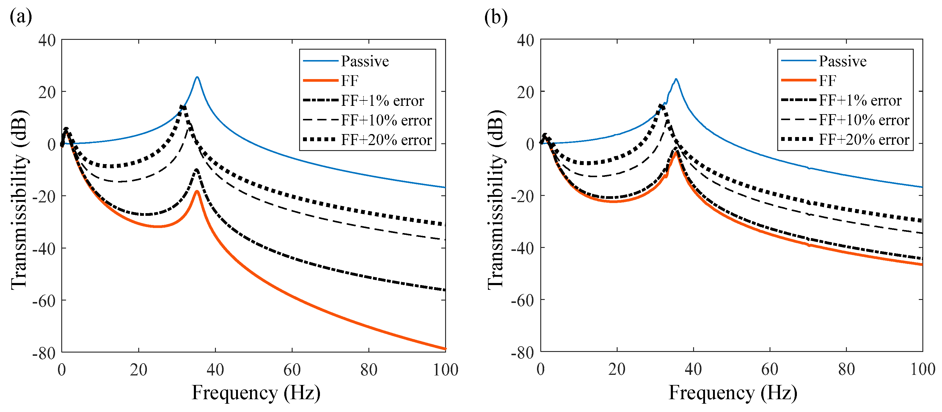
4.1. Influence of System Uncertainty on Feedforward

As can be seen from the previous section, the design of the feedforward controller is completely dependent on the system’s theoretical model. However, it is difficult to obtain an accurate theoretical model in practical engineering. Therefore, it is necessary to discuss the influence of system uncertainty on the feedforward controller. According to the controller structure in Figure 2, we can easily obtain the vibration transmission of the system after adding the feedforward controller independently without considering the feedback control loop, as presented in Figure 3. The red line in Figure 3 is obtained when the feedforward controller parameters exactly match the system parameters, which is able to offset the disturbance in almost the full band. Since the cutoff frequency of the feedforward controller is 2 Hz, vibration transmission from about 2 Hz has a vibration isolation effect.
However, the system parameters will change to some extent in practical engineering, resulting in the controller parameters and system parameters not matching accurately. For example, Figure 3 shows the transmissibility curves in the case of a 1%, 10%, and 20% system parameters error, i.e., c → 0.99c, k → 0.99k, and c → 0.9c, k → 0.9k, as well as c → 0.8c, k → 0.8k, respectively. It is obvious that the greater the error of system parameters, the worse the vibration isolation performance. By comparing Figure 3a,b, it can be seen that sensor noise will reduce the vibration isolation effect of feedforward control, and the higher the model accuracy, the more significant the reduction. But, even at 20% error of system parameters, the feedforward control still has a wide band vibration isolation performance. It, thus, makes sense to add a feedforward control loop to the controller design of the system with certain uncertainty.

4.2. Tolerance Analysis of Kalman Filter

The Kalman filter is the core of the feedback control loop, the accuracy of state estimation directly affects the isolation performance of the active vibration isolation system. Therefore, this section analyzes the estimation error of state variables for a system with uncertainty. Define the root mean square error as follows:
e r m s = i = 1 n ( z ^ i z i ) 2 n ,
where  z ^  represents the measured value of the system output or the estimated value of the system state variable.  z  is the corresponding true value. n is the number of samples. Since accelerometers are often used to detect vibration signals in the field of vibration control, acceleration is taken as the output of the system in this paper. Displacement and speed are the state variables. In order to better analyze the relationship between different dimensions, the normalized error is defined as follows:
e ¯ r m s = e r m s n / i = 1 n z i 2 .
In order to analyze the adaptability of the Kalman filter to the system with uncertainty, MATLAB/Simulink 2018b is used to simulate the state estimations of the Kalman filter. Acceleration is used as output in system modeling. The acceleration signal collected by the sensor is simulated by adding white noise to the real output of the system and used as the input of the Kalman filter. Since the variance of the noise signal measured by the sensor is known, the state estimation errors of the Kalman filter are analyzed by changing the covariance matrix corresponding to the system process noise. Assuming that the noise among state variables is independent of each other and the variances are q, the covariance matrix Q of process noise can be expressed as follows:
Q = q 0 0 q .
Similarly, this section also considers four system model cases: the exact matching of parameters, 1% error, 10% error, and 20% error. Sinusoidal voltage signals (amplitude 1 V) with the frequencies of 10 Hz and 25 Hz are input to the system, and the Kalman filter is used to estimate the acceleration, velocity, and displacement of the system. In order to better analyze the tolerance of the Kalman filter to system uncertainty, the Luenberger observer, which is completely based on theoretical models, is used for comparison. The estimation error results are shown in Figure 4. By comparing Figure 4a,b, It can be seen that the measurement error of acceleration at 10 Hz is large, while that at 25 Hz is small, which is caused by the frequency response characteristics of the system. The less responsive the system is, the more susceptible it is to noise. The Luenberger observer shows good tracking performance for the measurement outputs with different error sizes. However, the accuracy of the estimation of velocity and displacement mainly depends on the accuracy of the theoretical model. For example, when the model is perfectly matched, the estimation error is very small. When the model error is 10%, the normalized error of velocity and displacement is also about 10%.
For the Kalman filter, the larger the q value, the closer the estimated value is to the measured result, and the smaller the q value, the closer the estimated value is to the theoretical value. For example, for q = 1 × 10⁻⁶ (very small), when the model is accurate (matched, 1% error), the estimate of acceleration and velocity is very close to the true value, but when the model error is large (10% error, 20% error), the estimated error also increases. Therefore, the Kalman filter can achieve a good filtering effect for the measurement outputs by selecting the appropriate variance q. More importantly, when the model parameters of the Kalman filter differ from the actual system parameters, it can also achieve a more accurate estimation of the velocity. These are the keys for the Kalman filter to be applied to systems with uncertainty. In practical application, the appropriate variance q can be determined according to the filtering effect of the Kalman filter on the measured acceleration. However, the disadvantage is that the estimation of displacement by the Kalman filter depends on the model accuracy as much as the Luenberger observer.

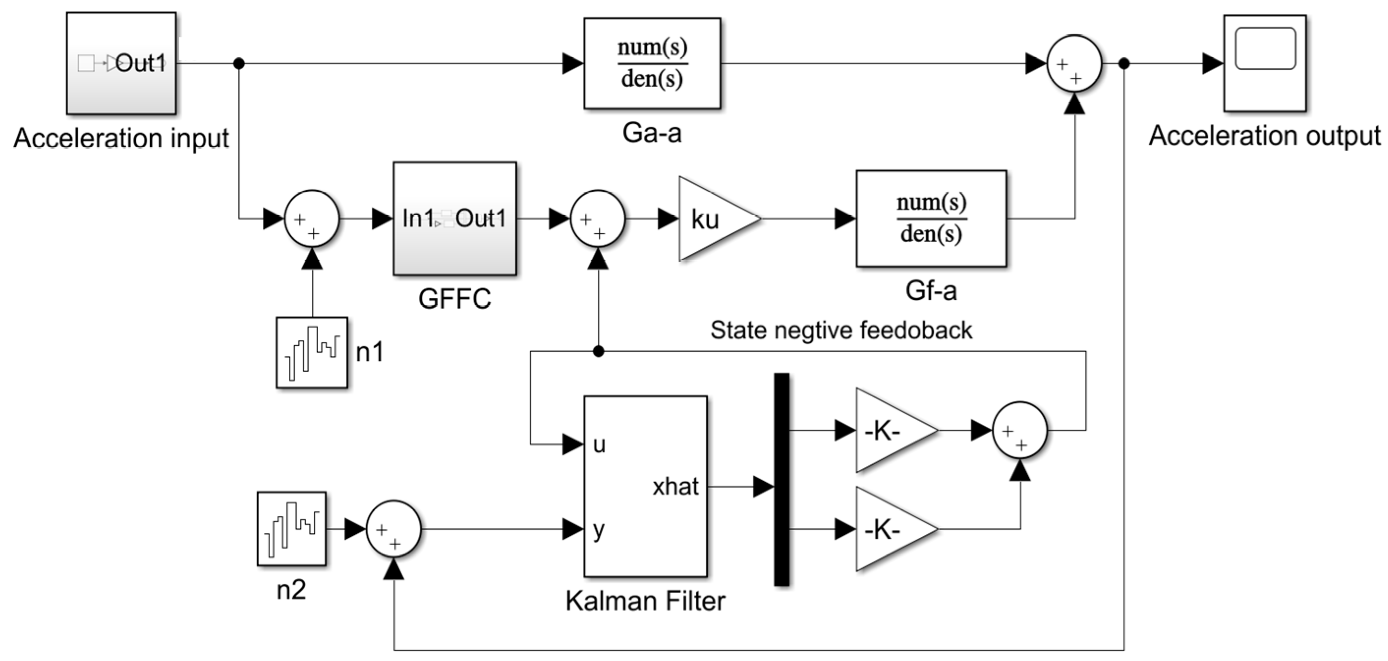
4.3. Performance Analysis of Proposed Composite Controller

In order to analyze the vibration isolation performance of the proposed ACC applied to the system with uncertainty, a simulation model of the composite controller is established according to Figure 2, as shown in Figure 5. In this paper, the LQR algorithm is used to optimize the value of state negative feedback gain. In order to obtain a better vibration isolation effect, the weight matrixes of state variables and control output are set as Q = [1000,0; 0,1000] and R = 1, respectively. Finally, the displacement negative feedback gain k1 is 0.06, and the velocity negative feedback gain k2 is 29.58. Since the gain of displacement negative feedback is very small and almost negligible, it is mainly the velocity negative feedback that plays a role.
According to the analysis results in Section 4.1 and Section 4.2, this section analyzes two cases where the model accuracy is a perfect match and the 20% error model. The variance q of the system process noise is discussed by taking 1 × 10⁻³ and 1 × 10⁻⁶, respectively. The vibration isolation performance without and with noise in the case of the matched model is illustrated in Figure 6a and Figure 6b, respectively, while Figure 6c,d depict the vibration isolation performance without and with noise in the case of the 20% error model. By comparing with Figure 6a,b and Figure 6c,d, respectively, the more accurate the model of the controller is, the more significant the vibration isolation effect is, which is mainly due to the disturbance compensation of the feedforward control. It is easy to see that the resonance peak is attenuated by adding the feedback control on the basis of the feedforward control. The reason is that adding a velocity negative feedback control is equivalent to increasing the damping of the system, so the system resonance is suppressed.
The effect of noise on the feedforward controller has been analyzed in Section 4.1. The sensor noise is amplified through the feedback control loop, which also affects the final control effect. Compared with Figure 6a,b, the proposed ACC has better tolerance on sensor noise than the completely model-based ACC (replacing the Kalman filter in the proposed ACC with the Luenberger observer). The main reason is that the Kalman filter has the function of both filtering and state estimation. As can be seen from Figure 6c,d, the influence of sensor noise on the proposed composite controller can be basically ignored under the 20% error model, but it has a great impact on the vibration isolation performance of the completely model-based ACC. Therefore, compared with the completely model-based ACC, the proposed ACC can effectively reduce the influence of sensor noise on the system.
Without considering the noise, the completely model-based ACC is worse than the proposed ACC, and even worse than the feedforward control alone at high frequencies. In the case of the matched model in Figure 6a, the poor vibration isolation effect of the completely model-based ACC still occurs. The main reason is that the control input of the feedback control loop is used to approximately replace the total input of the Luenberger observer/Kalman filter, resulting in a small deviation in the state estimation of the Luenberger observer, so the vibration isolation effect is poor. When the stiffness and damping of the actual system model change (reduced by 20%), it can be seen from Section 4.2 that the system velocity estimated by the Luenberger observer exhibits a large error, which is the main reason for the result in Figure 6c.
As can be seen from Figure 6, the proposed ACC can further reduce the resonance peak while maintaining the effect of the feedforward control, and the resonance peak is reduced more than the completely model-based ACC. The proposed ACC can not only show better control effects in matched models, but also achieve better vibration isolation effects in uncertain systems. The reason is that the Kalman filter revealed above all has a better tolerance for uncertainty and noise, and can achieve a more accurate estimate of the velocity of the system. Because of the influence of uncertainty in the theoretical estimation of the Kalman filter, the vibration isolation effect of q = 1×10⁻³ is slightly better than that of q = 1×10⁻⁶.

5. Experiments

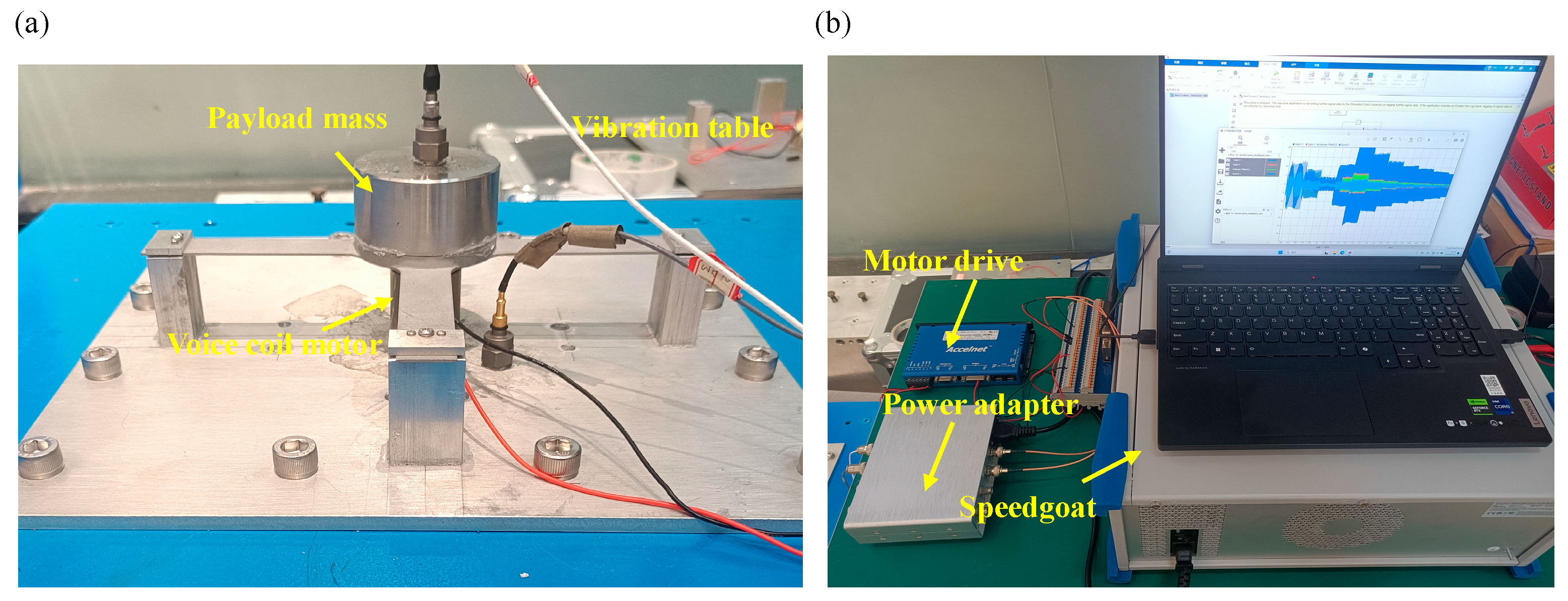
5.1. Experiments Setup

To prove the effectiveness of the proposed ACC, an SDOF isolation system is established, as shown in Figure 7a. A vibration table is used to generate external disturbance inputs. Accelerometers are used to detect the input signal of the system and the output signal of the load, which are used as inputs to the feedforward and feedback controllers, respectively. The acting element of the active vibration isolation system is the voice coil motor. The proposed ACC algorithm is achieved by a semi-physical simulation system (speedgoat), as shown in Figure 7b. The power adapter in Figure 7b is used to power the accelerometers. The output voltage of the controller drives the voice coil motor through the motor driver to realize active vibration isolation.

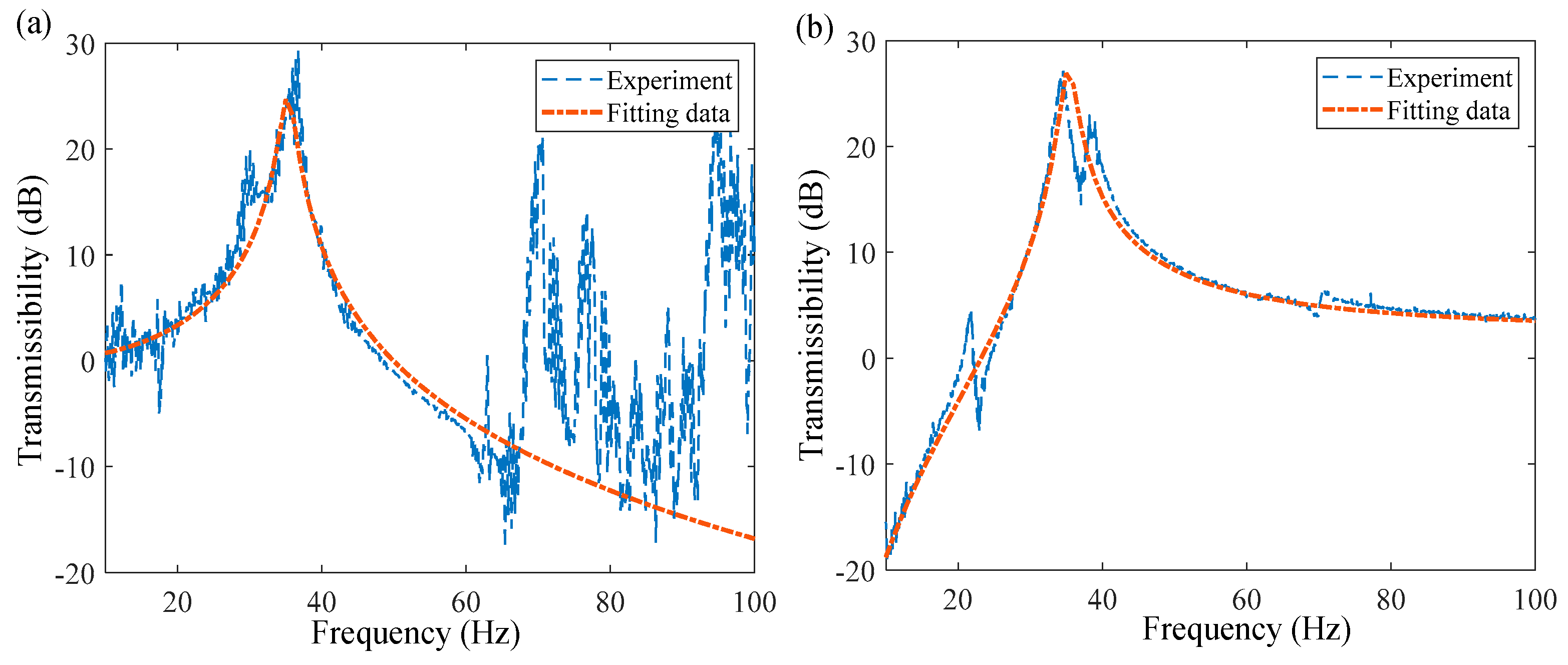
5.2. System Identification

To simulate an SDOF system, a mechanical system as shown in Figure 7a is constructed. Due to the flexible spring being replaced by a thin beam structure, there are some high-order modes which are not considered in this paper. System identification can effectively obtain main model information and reduce system uncertainty. Based on partial model information and partial measurable perturbations, vibration isolation can be further improved by cleverly designing the controller.
System identification includes two parts: (1) The transfer function of the acceleration response generated by the vibration table to the acceleration response of load (primary channel identification); (2) the transfer function of the output voltage of the controller to the acceleration response of load (secondary channel identification). The vibration transfer curve of the primary channel can be obtained by controlling the vibration table to generate 10–100 Hz sweeping vibration excitation, as presented in Figure 8a. It can be clearly seen that the natural frequency of the SDOF system is about 35 Hz. However, there are other formants in the measured curve. This is mainly caused by the measurement noise and the modes generated by the thin plate and beam structure, which are ignored in the identification process. The payload mass can be measured (0.76 kg). The stiffness and damping of the SDOF system can be obtained by fitting the vibration transfer curve of the primary channel with Equation (4) (k = 3.74 × 10⁴ N/m, c = 9.5), as shown by the red line in Figure 8a.
The transfer function from the output force of the voice coil motor to the acceleration of the load is presented in Equation (5). According to Equation (5), we assume that the transfer function ( G u a ) from the control output voltage to the acceleration of the load can be expressed as follows:
G u a = s 2 Y ( s ) U ( s ) = k u s 2 m s 2 + c s + k ,
where  k u  is regarded as the gain coefficient converted from the control output voltage to the output force of the voice coil motor. To obtain the gain coefficient  k u , a random voltage signal is sent to the real-time AO port of the speedgoat to drive the voice coil motor in the Simulink model, and then the load acceleration signal is collected by an accelerometer. Therefore, the measured vibration transfer curve of the secondary channel can be obtained according to the input and output signals of the secondary channel, as shown in Figure 8b. Similarly, the system parameters (m, c, and k) have been obtained, and  k u  can be obtained by fitting the corresponding measured vibration transfer function curve with Equation (39) ( k u  = 4.5). The fitting results are basically consistent with the measured results. Comparing Figure 8a,b, the system parameters of primary channel identification are basically correct.

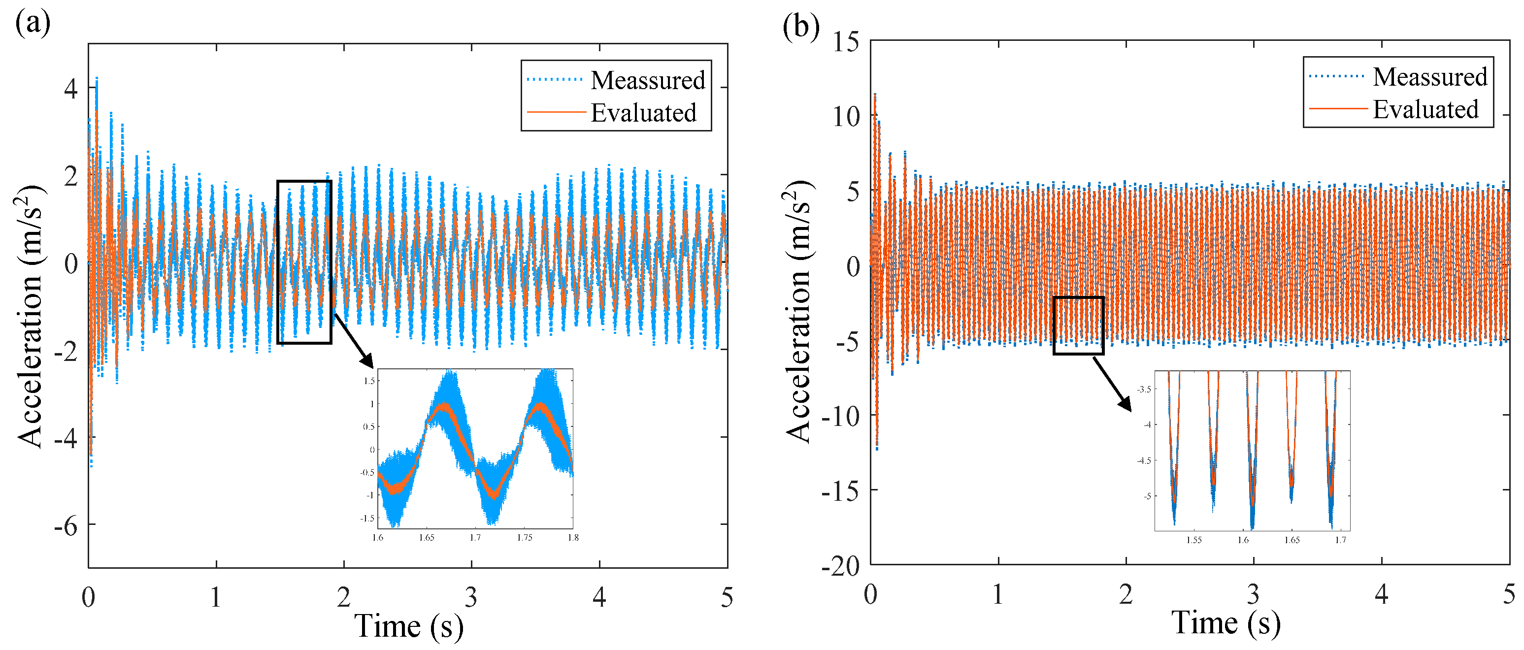
5.3. Kalman Filtering Effect

In the application of the Kalman filter, it is necessary to define the covariance matrixes of process noise and measurement noise. In fact, these covariance matrices are weight coefficients that weigh whether the observed output of the Kalman filter is closer to the measured result or the theoretical result. The process noise cannot be measured, so its covariance matrix can only be obtained by debugging during the experiments. But, the measurement noise can be directly obtained by an accelerometer, as shown in Figure 9. The mean of the measurement noise is −0.0056 and the variance is 0.0057, which approximately follows a normal distribution with zero mathematical expectation. In this paper, the covariance matrixes of process noise and measurement noise are Q= [5 × 10⁻⁵ 0; 0 5 × 10⁻⁵] and R = 0.0057, respectively.
By inputting the sinusoidal voltage signals of 10 Hz and 25 Hz to the voice coil motor driver, the load acceleration responses of the corresponding frequency are obtained, as presented in Figure 10. We can see that the Kalman filter can filter the noisy signal effectively without phase delay. Although the signal to noise ratio of the system response signal is small, the Kalman filter can also estimate the real response of the system relatively accurately (Figure 10a). Therefore, the Kalman filter can also accurately estimate the displacement and velocity state variables.

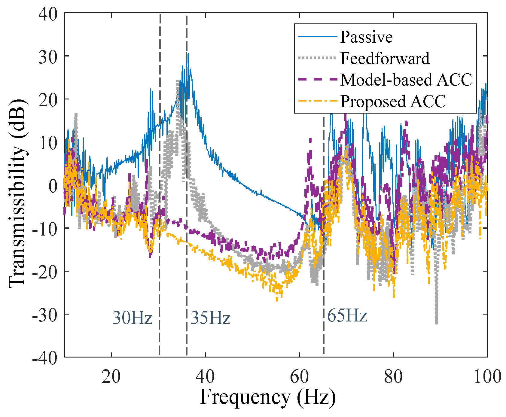
5.4. Vibration Isolation Performance

The active vibration isolation experiments of three different controllers were carried out in this section, including that of the feedforward control, completely model-based ACC, and proposed ACC. The Luenberger observer differs from the Kalman filter in that the state estimates of the Luenberger observer are based entirely on the theoretical model. It is suitable for comparison with the proposed composite controller based on the Kalman filter. Similarly, the vibration table outputs a sweeping vibration signal of 10–100 Hz, and accelerometers are adopted to measure the acceleration of the base and the load, respectively. Therefore, the vibration transmission curves for different control strategies are obtained, as shown in Figure 11. It can be clearly seen that the feedforward control has a certain isolation to the vibration in the full frequency range. However, because of the uncertainty of the system (parameter change, delay, unknown disturbance, etc.), the feedforward controller cannot fully compensate for the disturbance, especially the vibration near the resonance peak band.
Adding feedback control on the basis of feedforward can eliminate formant effectively. Comparing the ACC based on the Luenberger observer and the proposed ACC, they have basically the same vibration transmission before 30 Hz, but the vibration isolation effect of the proposed ACC after 30 Hz is obviously better than that of the completely model-based ACC. Such as, at the formant position (35 Hz), the completely model-based ACC reduces about 37 dB, and the proposed ACC reduces about 40.5 dB (increased by 3.5 dB). As presented in Figure 11, in the range of 30–65 Hz, the proposed method improves the vibration isolation efficiency by more than 5 dB on average compared with the model-based method. The experimental results presented in Figure 11 are basically consistent with the simulation results in Section 4.3. Due to the uncertainty and noise of the system, there is a large error in the state estimation of the Luenberger observer, which leads to the worse vibration isolation effect of the completely model-based ACC. The proposed ACC can effectively suppress the influence of noise and uncertainty, which can significantly suppress the vibration transmission near the resonance peak without affecting the effect of the feedforward control.

6. Conclusions

This paper provides an active composite control (ACC) strategy to improve the vibration isolation performance of the system with uncertainty. The proposed ACC integrates feedforward control based on known systems and feedback control based on the Kalman filter for systems with uncertainty. The feedforward controller is used to compensate for known disturbances to achieve low-frequency and wide-band vibration isolation. The feedback controller, which is a combination of the Kalman filter and LQR algorithm, is used to deal with the uncertainty of the system for obtaining an optimized control effect.
Further, the derivation and stability analyses of the proposed ACC algorithm are provided, and the influence of system uncertainty on vibration isolation performance based on the proposed ACC is analyzed. Several important conclusions are drawn from the analysis:
  • The feedforward controller designed with the known model can effectively obtain a lower and wider vibration isolation band.
  • The Kalman filter can effectively filter the output signal, and can accurately and effectively estimate the state (velocity) of the uncertain system.
  • Using more accurate estimated state feedback can achieve a better vibration isolation effect, and does not affect the performance of the feedforward controller.
  • The proposed ACC can not only reduce the influence of system uncertainty on the control effect, but also effectively suppress the influence of noise on the system.
Experimental verification is conducted and the experimental results show that the proposed ACC can effectively realize the low-frequency and wide-band vibration isolation for the system with uncertainty. Starting from 30 Hz, the vibration isolation performance of the proposed ACC with uncertainty is significantly improved than that of the completely deterministic model-based ACC (replacing the Kalman filter in the proposed ACC with the Luenberger observer). The resonance peak (35 Hz) is reduced by about 40.5 dB in the case of adopting the proposed ACC with uncertainty, which is about 3.5 dB better than the vibration isolation performance of the completely deterministic model-based ACC.

Author Contributions

Conceptualization, Z.Z. and Y.X.; methodology, Z.Z. and M.Z.; software, Z.Z. and M.Z.; validation, Z.Z., Y.X. and D.Y.; formal analysis, Z.Z. and Y.X.; investigation, Z.Z.; data curation, Z.Z. and Y.L.; writing—original draft preparation, Z.Z.; writing—review and editing, Z.Z. and Y.X.; visualization, Z.Z.; supervision, Y.X. and D.Y.; project administration, Y.X.; funding acquisition, Y.X. All authors have read and agreed to the published version of the manuscript.

Funding

This study is supported by the National Natural Science Foundation of China (Grant Nos. 51875569, 11991032).

Data Availability Statement

The data presented in this study are available upon reasonable request.

Conflicts of Interest

The authors declare no conflicts of interest.

References

  1. Cetinkaya, M.B.; Isci, M. Analysis of the Vibration Characteristics of a Leaf Spring System Using Artificial Neural Networks. Sensors 2022, 22, 4507. [Google Scholar] [CrossRef] [PubMed]
  2. Sjöberg, M.M.; Kari, L. Non-linear behavior of a rubber isolator system using fractional derivatives. Veh. Syst. Dyn. 2002, 37, 217–236. [Google Scholar] [CrossRef]
  3. Salvatore, A.; Carboni, B.; Chen, L.; Lacarbonara, W. Nonlinear dynamic response of a wire rope isolator: Experiment, identification and validation. Eng. Struct. 2021, 238, 112121. [Google Scholar] [CrossRef]
  4. Kovacic, I.; Brennan, M.J.; Waters, T.P. A study of a nonlinear vibration isolator with a quasi-zero stiffness characteristic. J. Sound Vib. 2008, 315, 700–711. [Google Scholar] [CrossRef]
  5. Carrella, A.; Brennan, M.J.; Waters, T.P. Static analysis of a passive vibration isolator with quasi-zero-stiffness characteristic. J. Sound Vib. 2007, 301, 678–689. [Google Scholar] [CrossRef]
  6. Ye, K.; Ji, J.C.; Brown, T. Design of a quasi-zero stiffness isolation system for supporting different loads. J. Sound Vib. 2020, 471, 115198. [Google Scholar] [CrossRef]
  7. Wang, M.; Hu, Y.; Sun, Y.; Ding, J.; Pu, H.; Yuan, S.; Zhao, J.; Peng, Y.; Xie, S.; Luo, J. An adjustable low-frequency vibration isolation Stewart platform based on electromagnetic negative stiffness. Int. J. Mech. Sci. 2020, 181, 105714. [Google Scholar] [CrossRef]
  8. He, K.; Li, Q.; Liu, L.; Yang, H. Active vibration isolation of ultra-stable optical reference cavity of space optical clock. Aerosp. Sci. Technol. 2021, 112, 106633. [Google Scholar] [CrossRef]
  9. Song, H.; Shan, X.; Hou, W.; Wang, C.; Sun, K.; Xie, T. A novel piezoelectric-based active-passive vibration isolator for low-frequency vibration system and experimental analysis of vibration isolation performance. Energy. 2023, 278, 127870. [Google Scholar] [CrossRef]
  10. Beijen, M.A.; Heertjes, M.F.; Butler, H.; Steinbuch, M. Disturbance feedforward control for active vibration isolation systems with internal isolator dynamics. J. Sound Vib. 2018, 436, 220–235. [Google Scholar] [CrossRef]
  11. Beijen, M.A.; Heertjes, M.F.; Van Dijk, J.; Hakvoort, W.B.J. Self-tuning MIMO disturbance feedforward control for active hard-mounted vibration isolators. Control Eng. Pract. 2018, 72, 90–103. [Google Scholar] [CrossRef]
  12. Paknejad, A.; Zhao, G.; Chesné, S.; Deraemaeker, A.; Collette, C. Design and optimization of a novel resonant control law using force feedback for vibration mitigation. Struct. Control Health Monit. 2022, 29, e2933. [Google Scholar] [CrossRef]
  13. Huang, C.; Yang, Y.; Dai, C.; Long, Z. Tracking-Differentiator-Based Position and Acceleration Feedback Control in Active Vibration Isolation with Electromagnetic Actuator. Actuators 2023, 12, 271. [Google Scholar] [CrossRef]
  14. Yan, T.H.; Pu, H.Y.; Chen, X.D.; Li, Q.; Xu, C. Integrated hybrid vibration isolator with feedforward compensation for fast high-precision positioning X/Y tables. Meas. Sci. Technol. 2010, 21, 065901. [Google Scholar] [CrossRef]
  15. Xu, A.; Xu, Z.; Zhang, H.; Wang, L.; He, S. An adaptive feed-forward active vibration isolation algorithm for input disturbance unbalanced MIMO systems. Signal Process. 2024, 217, 109346. [Google Scholar] [CrossRef]
  16. Zhao, G.; Paknejad, A.; Deraemaeker, A.; Collette, C. ∞ optimization of an integral force feedback controller. J. Vib. Control 2019, 25, 2330–2339. [Google Scholar] [CrossRef]
  17. Zhao, G.; Paknejad, A.; Raze, G.; Deraemaeker, A.; Kerschen, G.; Collette, C. Nonlinear positive position feedback control for mitigation of nonlinear vibrations. Mech. Syst. Signal Process. 2019, 132, 457–470. [Google Scholar] [CrossRef]
  18. Beijen, M.A.; Heertjes, M.F.; Butler, H.; Steinbuch, M. Mixed feedback and feedforward control design for multi-axis vibration isolation systems. Mechatronics 2019, 61, 106–116. [Google Scholar] [CrossRef]
  19. Wang, M.; Fu, S.; Ding, J.; Sun, Y.; Peng, Y.; Luo, J.; Pu, H. Analytical and experimental validation of vibration isolation system with complementary stiffness and composite control. Aerosp. Sci. Technol. 2023, 133, 108117. [Google Scholar] [CrossRef]
  20. Pu, H.; Fu, S.; Wang, M.; Fang, X.; Cai, Y.; Ding, J.; Sun, Y.; Peng, Y.; Xie, S.; Luo, J. Active vibration hybrid control strategy based on multi-DOFs piezoelectric platform. J. Intell. Mater. Syst. Struct. 2024, 35, 352–366. [Google Scholar] [CrossRef]
  21. Li, Y.; Wang, X.; Huang, R.; Qiu, Z. Active vibration and noise control of vibro-acoustic system by using PID controller. J. Sound Vib. 2015, 348, 57–70. [Google Scholar] [CrossRef]
  22. Zhang, S.; Schmidt, R.U.D.; Qin, X. Active vibration control of piezoelectric bonded smart structures using PID algorithm. Chin. J. Aeronaut. 2015, 28, 305–313. [Google Scholar] [CrossRef]
  23. Wang, L.; Liu, J.; Yang, C.; Wu, D. A novel interval dynamic reliability computation approach for the risk evaluation of vibration active control systems based on PID controllers. Appl. Math. Model. 2021, 92, 422–446. [Google Scholar] [CrossRef]
  24. Zhao, G.; Raze, G.; Paknejad, A.; Deraemaeker, A.; Kerschen, G.; Collette, C. Active tuned inerter-damper for smart structures and its ∞ optimisation. Mech. Syst. Signal Process. 2019, 129, 470–478. [Google Scholar] [CrossRef]
  25. Beijen, M.A.; Heertjes, M.F.; Butler, H.; Steinbuch, M. H ∞ feedback and feedforward controller design for active vibration isolators. IFAC-Pap. 2017, 50, 13384–13389. [Google Scholar] [CrossRef]
  26. Zhao, B.; Shi, W.; Tan, J. Design and Control of a Dual-Stage Actuation Active Vibration Isolation System. IEEE Access 2019, 7, 134556–134563. [Google Scholar] [CrossRef]
  27. Shen, Y.; Yao, W.; Wen, J.; He, H.; Chen, W. Adaptive Supplementary Damping Control of VSC-HVDC for Interarea Oscillation Using GrHDP. IEEE Trans. Power Syst. 2018, 33, 1777–1789. [Google Scholar] [CrossRef]
  28. Hakvoort, W.B.J.; Beijen, M.A. Filtered-error RLS for self-tuning disturbance feedforward control with application to a multi-axis vibration isolator. Mechatronics 2023, 89, 102934. [Google Scholar] [CrossRef]
  29. Batista, E.L.O.; Barghouthi, M.R.; Lopes, E.M.D.O. A Novel Adaptive Scheme to Improve the Performance of Feedforward Active Vibration Control Systems. IEEE/ASME Trans. Mechatron. 2022, 27, 2322–2332. [Google Scholar] [CrossRef]
  30. Xie, L.; Qiu, Z.; Zhang, X. Analysis and experiments of adaptive feedforward and combined vibration control system with variable step size and reference filter. Aerosp. Sci. Technol. 2017, 61, 109–120. [Google Scholar] [CrossRef]
  31. Wang, M.; Fang, X.; Wang, Y.; Ding, J.; Sun, Y.; Luo, J.; Pu, H. A dual-loop active vibration control technology with an RBF-RLS adaptive algorithm. Mech. Syst. Signal Process. 2023, 191, 110079. [Google Scholar] [CrossRef]
  32. Landau, I.D.; Airimitoaie, T.; Alma, M. IIR Youla-Kucera Parameterized Adaptive Feedforward Compensators for Active Vibration Control with Mechanical Coupling. IEEE Trans. Control Syst. Technol. 2013, 21, 765–779. [Google Scholar] [CrossRef]
  33. Airimitoaie, T.; Landau, I.D. Robust and Adaptive Active Vibration Control Using an Inertial Actuator. IEEE Trans. Ind. Electron. 2016, 63, 6482–6489. [Google Scholar] [CrossRef]
  34. Landau, I.D.E.; Melendez, R.; Airimitoaie, T.; Dugard, L. Beyond the delay barrier in adaptive feedforward active noise control using Youla–Kučera parametrization. J. Sound Vib. 2019, 455, 339–358. [Google Scholar] [CrossRef]
  35. Landau, I.D.E.; Constantinescu, A.; Rey, D. Adaptive narrow band disturbance rejection applied to an active suspension—an internal model principle approach. Automatica 2005, 41, 563–574. [Google Scholar] [CrossRef]
  36. Airimitoaie, T.; Landau, I.D. Combined adaptive feedback and feedforward compensation for active vibration control using Youla–Kučera parametrization. J. Sound Vib. 2018, 434, 422–441. [Google Scholar] [CrossRef]
  37. Wang, Y.P.; Sinha, A. Adaptive sliding mode control algorithm for a microgravity isolation system. Acta Astronaut. 1998, 43, 377–384. [Google Scholar] [CrossRef]
  38. Davis, L.; Hyland, D.; Yen, G.; Das, A. Adaptive neural control for space structure vibration suppression. Smart Mater. Struct. 1999, 8, 753. [Google Scholar]
  39. Deshpande, V.S.; Mohan, B.; Shendge, P.D.; Phadke, S.B. Disturbance observer based sliding mode control of active suspension systems. J. Sound Vib. 2014, 333, 2281–2296. [Google Scholar] [CrossRef]
  40. Kempf, C.J.; Kobayashi, S. Disturbance observer and feedforward design for a high-speed direct-drive positioning table. IEEE Trans. Control Syst. Technol. 1999, 7, 513–526. [Google Scholar] [CrossRef]
  41. Su, J.; Wang, L.; Yun, J.N. A design of disturbance observer in standard H ∞ control framework. Int. J. Robust Nonlinear Control 2015, 25, 2894–2910. [Google Scholar] [CrossRef]
  42. Han, J. From PID to Active Disturbance Rejection Control. IEEE Trans. Ind. Electron. 2009, 56, 900–906. [Google Scholar] [CrossRef]
  43. Li, J.; Zhang, L.; Li, S.; Su, J. A Time Delay Estimation Interpretation of Extended State Observer-Based Controller with Application to Structural Vibration Suppression. IEEE Trans. Autom. Sci. Eng. 2024, 21, 1965–1973. [Google Scholar] [CrossRef]
  44. Li, J.; Zhang, L.; Zhang, M.; Li, S.; Su, J.; Luo, L. Multi-modal vibration control for all-clamped plate subjected to periodic disturbances by ESO-based frequency-shaped LQR. Mech. Syst. Signal Process. 2023, 201, 110658. [Google Scholar] [CrossRef]
  45. Zhang, M.; Jing, X. Switching logic-based saturated tracking control for active suspension systems based on disturbance observer and bioinspired X-dynamics. Mech. Syst. Signal Process. 2021, 155, 107611. [Google Scholar] [CrossRef]
  46. Ai, C.; Guo, J.; Gao, W.; Chen, L.; Zhou, G.; Han, Z.; Kong, X. Active Disturbance Rejection Control With Linear Quadratic Regulator for Power Output of Hydraulic Wind Turbines. IEEE Access 2020, 8, 159581–159594. [Google Scholar] [CrossRef]
  47. Kalman, R.E.; Bucy, R. New results in linear filtering and prediction theory. J. Basic Eng. Trans. ASME Ser. D 1961, 83, 95–108. [Google Scholar] [CrossRef]
  48. Bandopadhya, D.; Njuguna, J. A Study on the Effects of Kalman Filter on Performance of IPMC-Based Active Vibration Control Scheme. IEEE Trans. Control Syst. Technol. 2010, 18, 1315–1324. [Google Scholar] [CrossRef]
  49. Papadimitriou, C.; Fritzen, C.; Kraemer, P.; Ntotsios, E. Fatigue predictions in entire body of metallic structures from a limited number of vibration sensors using Kalman filtering. Struct. Control Health Monit. 2011, 18, 554–573. [Google Scholar] [CrossRef]
  50. Erazo, K.; Sen, D.; Nagarajaiah, S.; Sun, L. Vibration-based structural health monitoring under changing environmental conditions using Kalman filtering. Mech. Syst. Signal Process. 2019, 117, 1–15. [Google Scholar] [CrossRef]
  51. Hamel, T.; Samson, C. Position estimation from direction or range measurements. Automatica 2017, 82, 137–144. [Google Scholar] [CrossRef]
Figure 1. Schematic of an SDOF system and its control strategy.
Actuators 13 00334 g001
Figure 2. Block diagram of the hybrid controller structure.
Actuators 13 00334 g002
Figure 3. The influence of parameter uncertainty on feedforward (FF) control. (a) No noise. (b) With noise.
Actuators 13 00334 g003
Figure 4. Estimation errors of Kalman filter. (a) f = 10 Hz. (b) f = 25 Hz.
Actuators 13 00334 g004
Figure 5. Simulink simulation of the proposed composite controller.
Actuators 13 00334 g005
Figure 6. Vibration isolation effect of the proposed composite control. (a) Matched model without noise. (b) Matched model with noise. (c) The 20% error model without noise. (d) The 20% error model with noise.
Actuators 13 00334 g006
Figure 7. Experiments setup. (a) SDOF system prototype. (b) Control devices.
Actuators 13 00334 g007
Figure 8. Vibration transmissibility tests. (a) Primary channel. (b) Secondary channel.
Actuators 13 00334 g008
Figure 9. The measured noise signal of the accelerometer.
Actuators 13 00334 g009
Figure 10. The evaluated accelerations by Kalman filter. (a) 10 Hz. (b) 25 Hz.
Actuators 13 00334 g010
Figure 11. Experiment results of active vibration isolation performance.
Actuators 13 00334 g011
Disclaimer/Publisher’s Note: The statements, opinions and data contained in all publications are solely those of the individual author(s) and contributor(s) and not of MDPI and/or the editor(s). MDPI and/or the editor(s) disclaim responsibility for any injury to people or property resulting from any ideas, methods, instructions or products referred to in the content.

