Nonlinear Robust Control for Missile Unsupported Random Launch Based on Dynamic Surface and Time Delay Estimation

Abstract

Due to the difficulty in ensuring launch safety under unfavorable launch site conditions, restrictions regarding the selection of launch sites significantly weaken the maneuverability of the unsupported random vertical launch (URVL) mode. In this paper, a nonlinear robust control strategy is proposed to control the missile attitude by actively adjusting the oscillation of the launcher through the hydraulic actuator, enhancing the launching safety and the adaptability of the VMLS to the launching site. Firstly, considering the interaction among the launch canister, adapters, and missile, a 6-DOF dynamic model of the launch system is established, in combination with the dynamics of the hydraulic actuator. Then, in order to facilitate the nonlinear controller design, the seventh-order state-space equation is constructed, according to the dynamic model of the launch system. Subsequently, in view of the problem of “differential explosion” in the backstepping controller design of the seventh-order nonlinear system, a nonlinear dynamic surface control (DSC) framework is proposed. Meanwhile, the time delay estimation (TDE) technique is introduced to suppress the influence of the complex nonlinearities of the launch system on the missile attitude control, and a nonlinear robust control (NRC) is introduced to attenuate the TDE error. Both of these are integrated into the DSC framework, which can achieve asymptotic output tracking. Finally, numerical simulations are conducted to validate the superiority of the proposed control strategy in regards to missile launch response control.

1. Introduction

In the last decade or so, the unsupported random vertical launch (URVL) mode has become an important research direction in the field of vehicular missile launching due to its advantages in regards to survivability and rapid strike capability [1,2,3,4,5,6,7,8,9,10,11]. URVL refers to the process of missile launch no longer relying on a predetermined launching site, but rather randomly selecting a site for launch [2]. This means that the launch dynamic responses of the missile and the launcher are not only determined by their own structure and the combustion effect of the propellant, but also influenced by the dynamic response of the launching site. The drastic deformation of the launching site can cause instability of the launch system, missile vibration, and even excessive oscillation, leading to launch security problems [3]. In order to improve the adaptability of the launch system to the site, many scholars have studied the dynamic mechanism and dynamic response characteristics of the launch process from the perspective of improving the structural design of the launch system, including launch dynamic modeling and rapid simulation calculation methods [4,5,6,7], sensitivity analysis methods of influencing factors during the launch process [8], and dynamics response simulation methods of concrete sites [9,10,11]. However, this way of thinking, which attempts to suppress and attenuate the instability of the launch platform by changing the system structure and material properties, might increase the design difficulty and cost but ultimately bring limited benefits.

The proposal to actively regulate the launcher oscillation through the hydraulic actuator used for the erection of the launch canister and then suppress the missile oscillation is a creative attempt to improve the launching site adaptability of the unsupported random launching process. However, the launch dynamics are very complex, including the dynamic coupling between the site and launch platform; the interactions between the launch canister, adapters, and missile; the flexibility of the structure; and unknown external disturbances. These dynamic characteristics seriously affect the attitude control of the missile, resulting in the PID controller commonly used in engineering being insufficient to meet the specified performance and safety requirements. Therefore, it is necessary to analyze the influence mechanism of control input on missile attitude, establish the mathematical model and state-space equation of launch dynamics, and then design a nonlinear controller to control the missile attitude.

The establishment of an accurate mathematical model for launch dynamics requires consideration of the load transfer effects between the launch canister, adapters, and missile [12,13,14,15,16], which means that the state-space equation for missile attitude control through the hydraulic actuator must be high-order, and the system is modeled with highly nonlinearities and uncertainties. The use of backstepping control techniques is necessary to deal with the mismatched nonlinearities in the model, but the design process will become extremely complex due to the “differential explosion” problem in higher-order systems. To address this problem, the dynamic surface control (DSC) method was proposed in References [17,18,19,20], and satisfactory results were achieved by employing a first-order low-pass filter to construct a virtual control input to simplify the differential derivation. Zhang et al. [21] addressed the problem of controlling a multi-degree-of-freedom electro-hydraulic robotic arm by considering the dynamics of the hydraulic actuator and utilized the adaptive DSC method to achieve stabilization of the closed-loop system without velocity feedback. Gao et al. [22] used DSC as a master controller and combined it with adaptive dynamic programming for precise motion control of a quadrotor under unknown disturbances. However, due to the existence of filtering error, the DSC method can only guarantee the semi-global bounded stabilization of the tracking error. Yang et al. [23] proposed a smooth nonlinear filter for the DSC method, which can guarantee the semi-global asymptotic stabilization of the tracking error.

The simplification of the launch dynamic model ignores the mathematical description of complex factors such as the dynamic deformation of the launching site, flexibility of the vehicle structure, and launch vibration. At the same time, the attitude tracking of the missile is also significantly affected by internal disturbances caused by the friction of the actuator and the nonlinearities of the servo valve. Therefore, the method of controlling the launch response solely through DSC is still incomplete. In order to inhibit the impact of disturbances and uncertainties on the control performance, several effective solutions have been proposed in recent years, including nonlinear disturbance observer (NDO) [24,25], extended state observer (ESO) [26,27,28,29], and time delay estimation control (TDC) [30]. The TDC derived from time delay estimation (TDE) technology is known for its simple structure and good robustness. Its core concept is to use the delay dynamics of the system to estimate the unknown dynamics [31,32]. In recent years, the TDC has been widely used for motion control in the presence of uncertainties, nonlinearities, and unknown external disturbances. Despite the fact that TDC is simple and practical, it yields significant estimation errors at the low sampling frequencies of the system signals and theoretically only guarantees bounded stabilization of the system error. Therefore, Jin et al. [33,34,35,36] have combined TDC with higher-order sliding mode controllers to ensure that the tracking error of the system converges to zero in the presence of disturbances. However, this approach requires higher-order derivatives of the state variables and is difficult to be generalize to controller design for higher-order systems.

Inspired by the above problems and solutions, this article focuses on the control problem of missile attitude during the process of unsupported random vertical launch (URVL). Firstly, considering the dynamics of the hydraulic actuator, a 6-DOF dynamic model of the launch system, which is suitable for derivation of the state-space equation, is established. Subsequently, a seventh-order state-space equation is derived through mathematical simplification. In order to facilitate the seventh-order backstepping design and avoid the influence of the “differential explosion” problem, the smooth nonlinear filters are used to form the virtual control inputs to simplify differential derivation and eliminate the effect of filtering errors on system stability. To address the impact of modeling errors caused by model simplification, dynamic deformation of the site, flexibility of the vehicle structure, launch vibration, uncertain nonlinearities of the hydraulic system, and external forces on control performance, the TDE technique is used to estimate the lumped disturbances resulting from the combination of the above mentioned factors. Additionally, the smooth nonlinear robust terms are introduced during the controller design process to further eliminate the TDC error and ensure the asymptotic convergence of the system error. Finally, the superiority of the proposed controller is verified through the simulation of launch dynamic response control.

The main contributions of this article are summarized as follows:

(1) A nonlinear robust control strategy is proposed to control the missile attitude by actively adjusting the oscillation of the launcher through the hydraulic actuator, enhancing the launching safety and the adaptability of the VMLS to the launching site.

(2) The seventh-order state-space equation is constructed according to the dynamic model of the launch system to facilitate the nonlinear controller design, and the problem of “differential explosion” in the backstepping controller design of the seventh-order nonlinear system is circumvented by introducing a nonlinear dynamic surface control (DSC) framework.

(3) The time delay estimation and nonlinear robust control are integrated with the nonlinear DSC framework, which can suppress the influence of the complex nonlinearities of the launch system on the missile attitude control and can achieve asymptotic output tracking.

2. Problem Description and System Modeling

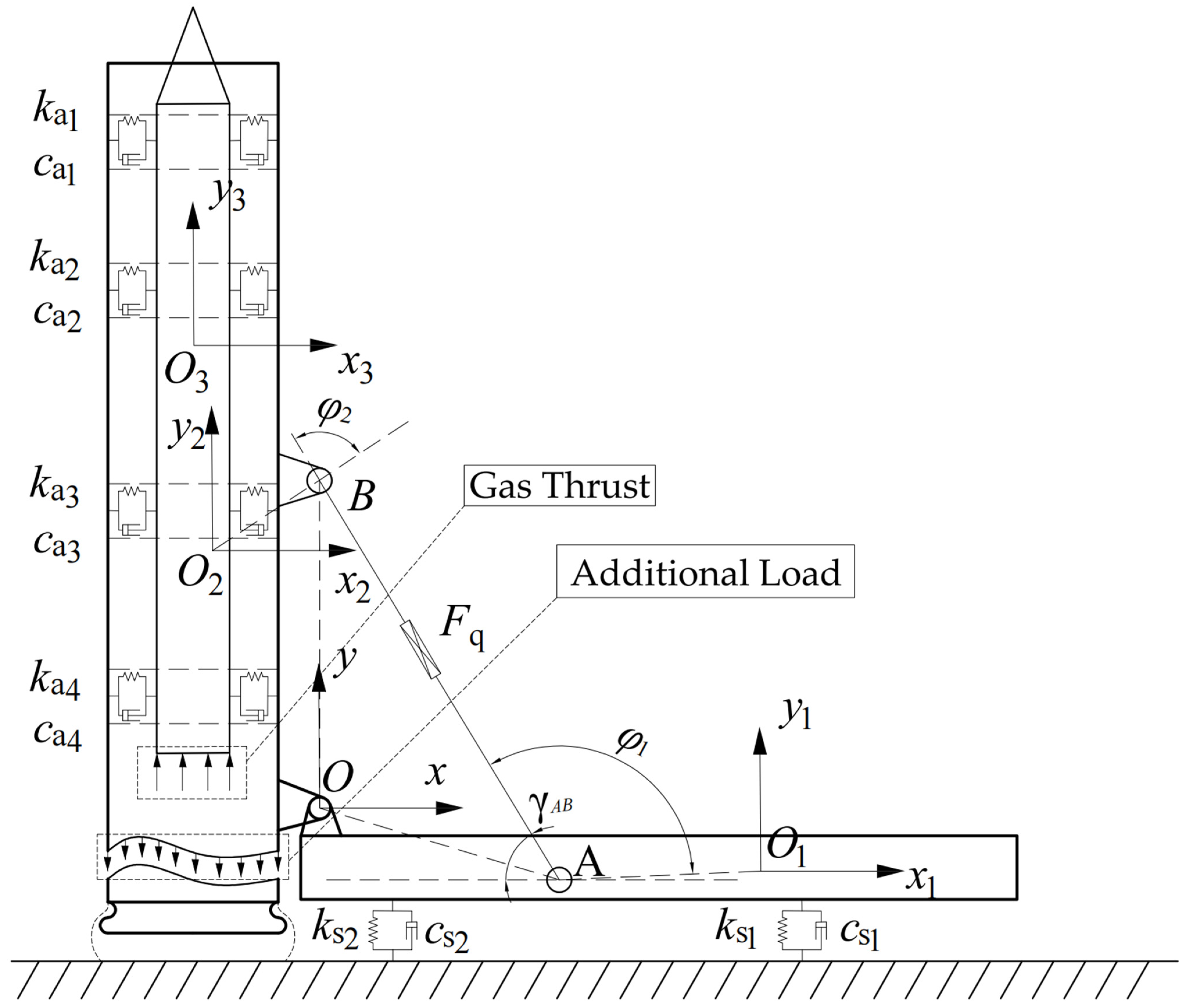
2.1. Unsupported Random Vertical Launch Dynamics Modeling

The typical multi-rigid-body dynamic model of a vehicular missile launching system (VMLS) is shown in Figure 1, including three rigid-body objects: the vehicle frame, the launch canister, and the missile. According to the conclusion of study [37], before leaving the launch canister, the change in the missile pitch angle is more obvious. The change in the yaw angle, the yaw angular velocity and roll angle, and the roll angular velocity is extremely small, and the load transfer of the launch system is mainly reflected in the plane perpendicular to the direction of the pitch angle velocity vector. Therefore, the multi-rigid-body dynamic model mentioned in this paper ignores the motion in the direction of the pitch angle velocity vector and only considers the plane rigid-body dynamics.

The vehicle frame is supported by front and rear outriggers, and the equivalent stiffness and damping of the front and rear outriggers are $k_{\mathrm{s}1}$, $k_{\mathrm{s}2}$, $c_{\mathrm{s}1}$, and $c_{\mathrm{s}2}$, respectively. The vehicle frame and launch canister are hinged at point O, and a hydraulic actuator is installed between the lower fulcrum A of the frame and the upper fulcrum B of the launch canister. The force of the hydraulic actuator $F_{\mathrm{q}}$ is calculated from the dynamic equation mentioned later. The load is transmitted between the missile and the launch canister via interference fitted adapters. Taking the four adapters as an example and simplifying the mechanical behavior of the adapters on the missile and the launch canister into spring-damped systems, the equivalent stiffness and damping of the $n$-th adapter ($n=1,2,3,4$) are $k_{\mathrm{a}n}$ and $c_{\mathrm{a}n}$. During the launching process, the gas pressure generated by the gas generator exerts an equivalent thrust on the base of the missile as $F_{\mathrm{t}}$. The gas pressure is transferred to the adaptive base, which pulls the launch canister downward with an additional load of $F_l$.

According to the structural characteristics of the launching system and the launching principle, the displacement $R_{x1}$ of the vehicle frame in the horizontal direction during the launching process is extremely small, and this degree of freedom will be neglected. Due to the rotational constraint between the launch canister and the frame, according to the theory of plane rigid-body dynamics, the independent degrees of freedom of the system are six, including the vertical displacement $R_{y1}$ and rotation angle ${\theta }_1$ of the vehicle frame; the rotation angle ${\theta }_2$ of the launch canister; and the horizontal displacement $R_{x3}$, vertical displacement $R_{y3}$, and rotation angle ${\theta }_3$ of the missile body (the corner markers 1, 2, and 3 represent the numbers of the rigid bodies, i.e., the vehicle frame, the launch canister, and the missile).

According to the principle of virtual work and Lagrangian dynamics, the system dynamic equation related to generalized coordinates can be obtained as follows:

$$M{\ddot{q}}^T=Q_{\mathrm{e}}+Q_{\mathrm{c}},$$

(1)

where $M$ is the mass matrix of the system, $Q_{\mathrm{e}}$ is the generalized external force associated with the generalized coordinates, $Q_{\mathrm{c}}$ is the generalized constraint associated with the generalized coordinates, and $q$ is the generalized coordinate of the system, which can be expressed as

$$q=\left[\begin{array}{cccccccc}{R}_{y1}& {\theta }_1& {\theta }_2& R_{x3}& R_{y3}& {\theta }_3& R_{x2}& R_{y2}\end{array}\right].$$

(2)

Referring to the modeling process of References [12,13], the dependent coordinates can be expressed in terms of independent coordinates according to Equation (1), and the 6-DOF launch dynamic equation that is only related to independent coordinates is obtained as follows:

$$\overline{M}{\ddot{q}}_{\mathrm{i}}^T=\overline{Q},$$

(3)

where $q_{\mathrm{i}}$ is the independent generalized coordinate of the system, which can be expressed as

$$q_{\mathrm{i}}=\left[\begin{array}{cccccc}{R}_{y1}& {\theta }_1& {\theta }_2& R_{x3}& R_{y3}& {\theta }_3\end{array}\right].$$

(4)

$\overline{M}$ can be denoted as

$$\overline{M}=\left[\begin{array}{cccccc}{m}_1+m_2\hfill & {\overline{m}}_{12}\hfill & -{\overline{m}}_{13}\hfill & 0\hfill & 0\hfill & 0\hfill \\ {\overline{m}}_{21}\hfill & {\overline{J}}_1\hfill & {\overline{m}}_{23}\hfill & 0\hfill & 0\hfill & 0\hfill \\ -{\overline{m}}_{31}\hfill & {\overline{m}}_{32}\hfill & {\overline{J}}_2\hfill & 0\hfill & 0\hfill & 0\hfill \\ 0\hfill & 0\hfill & 0\hfill & m_3\hfill & 0\hfill & 0\hfill \\ 0\hfill & 0\hfill & 0\hfill & 0\hfill & m_3\hfill & 0\hfill \\ 0\hfill & 0\hfill & 0\hfill & 0\hfill & 0\hfill & J_3\hfill \end{array}\right],$$

(5)

where ${\overline{m}}_{12}$, ${\overline{m}}_{21}$, ${\overline{m}}_{13}$, ${\overline{m}}_{31}$, ${\overline{m}}_{23}$, ${\overline{m}}_{32}$, ${\overline{J}}_1$, and ${\overline{J}}_2$ can be denoted, respectively, as

$${\overline{m}}_{12}={\overline{m}}_{21}=m_2({\overline{x}}_1\cos {\theta }_1-{\overline{y}}_1\sin {\theta }_1),$$

(6)

$${\overline{m}}_{13}={\overline{m}}_{31}=m_2({\overline{x}}_2\cos {\theta }_2-{\overline{y}}_2\sin {\theta }_2),$$

(7)

$$\begin{array}{l}{\overline{m}}_{23}={\overline{m}}_{32}=-m_2({\overline{x}}_1\sin {\theta }_1+{\overline{y}}_1\cos {\theta }_1)({\overline{x}}_2\sin {\theta }_2+{\overline{y}}_2\cos {\theta }_2)\\ -m_2({\overline{x}}_1\cos {\theta }_1-{\overline{y}}_1\sin {\theta }_1)({\overline{x}}_2\cos {\theta }_2-{\overline{y}}_2\sin {\theta }_2)\end{array},$$

(8)

$${\overline{J}}_1=J_1+m_2{({\overline{x}}_1\sin {\theta }_1+{\overline{y}}_1\cos {\theta }_1)}^2+m_2{({\overline{x}}_1\cos {\theta }_1-{\overline{y}}_1\sin {\theta }_1)}^2,$$

(9)

$${\overline{J}}_2=J_2+m_2{({\overline{x}}_2\sin {\theta }_2+{\overline{y}}_2\cos {\theta }_2)}^2+m_2{({\overline{x}}_2\cos {\theta }_2-{\overline{y}}_2\sin {\theta }_2)}^2.$$

(10)

$m_1$, $m_2$, and $m_3$ are the mass values of the vehicle body, the launch canister, and the missile, respectively. $J_1$, $J_2$, and $J_3$ are the moment of inertia of the vehicle body, the launch canister, and the missile, respectively. ${\overline{x}}_1$ and ${\overline{y}}_1$ are the initial horizontal and vertical coordinates of the center of mass of the frame. ${\overline{x}}_2$ and ${\overline{y}}_2$ are the initial horizontal and vertical coordinates of the center of mass of the launch canister. $\overline{Q}$ can be denoted as

$$\overline{Q}=\left[\begin{array}{c}{\overline{F}}_1+F_{\mathrm{s}1\_1}+F_{\mathrm{s}1\_2}-m_{1}g+F_{\mathrm{a}y2}+F_{\mathrm{f}y2}-F_l-m_{2}g\\ {\overline{F}}_2+M_{\mathrm{s}1\_1}+M_{\mathrm{s}1\_2}+M_{\mathrm{q}1}+({\overline{x}}_1\sin {\theta }_1+{\overline{y}}_1\cos {\theta }_1){\overline{F}}_3+({\overline{x}}_1\cos {\theta }_1-{\overline{y}}_1\sin {\theta }_1){\overline{F}}_4\\ {\overline{F}}_5+M_{\mathrm{q}2}+M_{\mathrm{a}2}-({\overline{x}}_2\sin {\theta }_2+{\overline{y}}_2\cos {\theta }_2){\overline{F}}_3-({\overline{x}}_2\cos {\theta }_2-{\overline{y}}_2\sin {\theta }_2){\overline{F}}_4+d_{3\mathrm{fa}}\\ -F_{\mathrm{t}3}\sin {\theta }_3+F_{\mathrm{a}x3}+F_{fx3}+d_{2\mathrm{f}}\\ -m_{3}g+F_{\mathrm{t}3}\cos {\theta }_3+F_{\mathrm{a}y3}+F_{\mathrm{f}y3}\\ M_{\mathrm{a}3}+d_{1\mathrm{f}}\end{array}\right],$$

(11)

where $d_{1\mathrm{f}}$ and $d_{2\mathrm{f}}$ are the disturbance terms affecting the missile oscillation and lateral motion, respectively; $d_{3\mathrm{fa}}$ is the disturbance term affecting the launcher canister oscillation, which contains modeling errors, the deformation of launching site, and the structural flexibility. ${\overline{F}}_1$, ${\overline{F}}_2$, ${\overline{F}}_3$, ${\overline{F}}_4$, and ${\overline{F}}_5$, respectively, can be denoted as

$${\overline{F}}_1=-m_2[-({\overline{x}}_1\sin {\theta }_1+{\overline{y}}_1\cos {\theta }_1){\dot{\theta }}_1^2+({\overline{x}}_2\sin {\theta }_2+{\overline{y}}_2\cos {\theta }_2){\dot{\theta }}_2^2],$$

(12)

$$\begin{array}{c}{\overline{F}}_2=m_2({\overline{x}}_1\sin {\theta }_1+{\overline{y}}_1\cos {\theta }_1)({\overline{x}}_2\cos {\theta }_2-{\overline{y}}_2\sin {\theta }_2){\dot{\theta }}_2^2\\ \hspace{1em} -m_2({\overline{x}}_1\cos {\theta }_1-{\overline{y}}_1\sin {\theta }_1)({\overline{x}}_2\sin {\theta }_2+{\overline{y}}_2\cos {\theta }_2){\dot{\theta }}_2^2\end{array},$$

(13)

$${\overline{F}}_3=F_{\mathrm{q}2}\cos {\gamma }_{AB}-F_{\mathrm{a}x2}-F_{\mathrm{f}x2},$$

(14)

$${\overline{F}}_4=F_{\mathrm{q}2}\sin {\gamma }_{AB}+F_{\mathrm{a}y2}+F_{\mathrm{f}y2}-F_{\mathrm{l}2}-m_{2}g,$$

(15)

$$\begin{array}{c}{\overline{F}}_5=m_2({\overline{x}}_1\cos {\theta }_1-{\overline{y}}_1\sin {\theta }_1)({\overline{x}}_2\sin {\theta }_2+{\overline{y}}_2\cos {\theta }_2){\dot{\theta }}_1^2\\ \hspace{1em} -m_2({\overline{x}}_1\sin {\theta }_1+{\overline{y}}_1\cos {\theta }_1)({\overline{x}}_2\cos {\theta }_2-{\overline{y}}_2\sin {\theta }_2){\dot{\theta }}_1^2\end{array}.$$

(16)

$F_{\mathrm{s}1\_1}$ and $F_{\mathrm{s}1\_2}$ are the support forces of the front and rear outriggers on the vehicle body, respectively, which are expressed as

$$\left\{\begin{array}{c}{F}_{\mathrm{s}1\_1}=k_{\mathrm{s}1}{d}_{\mathrm{s}1}+c_{\mathrm{s}1}{\dot{d}}_{\mathrm{s}1}\\ F_{\mathrm{s}1\_2}=k_{\mathrm{s}2}{d}_{\mathrm{s}2}+c_{\mathrm{s}2}{\dot{d}}_{\mathrm{s}2}\end{array}\right.,$$

(17)

where $d_{\mathrm{s}1}$ and $d_{\mathrm{s}2}$ are the deformations of the front and rear outriggers, respectively. $M_{\mathrm{s}1\_1}$ and $M_{\mathrm{s}1\_2}$ are the torques of the front and rear outriggers on the frame, respectively, denoted as

$$\left\{\begin{array}{c}{M}_{\mathrm{s}1\_1}=F_{\mathrm{s}1\_1}{L}_{\mathrm{s}1}\\ M_{\mathrm{s}1\_2}=F_{\mathrm{s}1\_2}{L}_{\mathrm{s}2}\end{array}\right.,$$

(18)

where $L_{\mathrm{s}1}$ and $L_{\mathrm{s}2}$ are the distances of the front and rear outriggers from the center of mass of the frame, respectively.

$M_{\mathrm{q}1}$ and $M_{\mathrm{q}2}$ are the moments acting on the frame and launch canister by the hydraulic actuator, respectively, denoted as

$$\left\{\begin{array}{c}{M}_{\mathrm{q}1}=F_{\mathrm{q}}{L}_{O_{1}A}\sin {\phi }_1\\ M_{\mathrm{q}2}=F_{\mathrm{q}}{L}_{O_{2}B}\sin {\phi }_2\end{array}\right.,$$

(19)

where $L_{O_{1}A}$ is the distance between point $O_1$ and point $A$; $L_{O_{2}B}$ is the distance between point $O_2$ and point $B$. ${\phi }_1$ is the angle between the line connecting point A and point B and the line connecting point A and the center of mass $O_1$ of the frame. ${\phi }_2$ is the angle between the line connecting point B and point A and the line connecting point B and the center of mass $O_2$ of the launcher.

$F_{\mathrm{a}x2}$ and $F_{\mathrm{a}y2}$ are the horizontal and vertical forces of the adapters on the launch canister, respectively, and $F_{\mathrm{a}2}$ is their vector sum, $F_{\mathrm{a}2}={\displaystyle \sum _{n=1}^4{F}_{\mathrm{a}2n}}$. $F_{\mathrm{a}2n}$ is the force of the $n$-th adapter on the launch canister, denoted by

$$F_{\mathrm{a}2n}=\left\{\begin{array}{ll}{k}_{\mathrm{a}n}(x_{\mathrm{a}n}+d_{\mathrm{o}})\hfill & x_{\mathrm{a}n}>d_{\mathrm{o}}\hfill \\ 2k_{\mathrm{a}n}{x}_{\mathrm{a}n}\hfill & -d_{\mathrm{o}}\le x_{\mathrm{a}n}\le d_{\mathrm{o}}\hfill \\ k_{\mathrm{a}n}(x_{\mathrm{a}n}-d_{\mathrm{o}})\hfill & x_{\mathrm{a}n}<-d_{\mathrm{o}}\hfill \end{array}\right.,$$

(20)

where $k_{\mathrm{a}n}=k_{\mathrm{l}}\pi D{h}_n(t)$ is calculated from the linear radial stiffness $k_{\mathrm{l}}$ per unit area of the adapter, the inner diameter $D$ of launch canister, and the axial contact length $h_n(t)$ between the n-th adapter and the inner wall of the launch canister. $d_{\mathrm{o}}$ is the amount of interference between the adapter and the launch canister. $x_{\mathrm{a}n}$ is the horizontal displacement of the missile relative to the launch canister at the centerline position of the n-th adapter, which can be denoted as

$$x_{\mathrm{a}n}=R_{x3}-z_n{\theta }_3-[R_{x2}+{\overline{x}}_{\mathrm{a}2n}\cos {\theta }_2-({\overline{y}}_{\mathrm{a}2n}+z_{\mathrm{v}})\sin {\theta }_2],$$

(21)

where ${\overline{x}}_{\mathrm{a}2n}$ and ${\overline{y}}_{\mathrm{a}2n}$ are the horizontal and vertical local coordinates of the launch canister at the n-th adapter, respectively, $z_n$ is the distance between the $n$-th adapter centerline and the center of mass of the missile along the axial direction of the canister, and $z_{\mathrm{v}}$ is the displacement of the missile relative to the launch canister along the axial direction. $F_{\mathrm{a}x3}$ and $F_{\mathrm{ay}3}$ are the horizontal and vertical forces of the adapters on the missile, respectively, and $F_{\mathrm{a}3}$ is their vector sum, $F_{\mathrm{a}3}={\displaystyle \sum _{n=1}^4{F}_{\mathrm{a}3n}=}-F_{\mathrm{a}2}$.

$F_{\mathrm{f}x2}$ and $F_{\mathrm{f}y2}$ are the friction components of the adapters on the launch canister in the horizontal and vertical directions, respectively, and $F_{\mathrm{f}2}$ is their vector sum, $F_{\mathrm{f}2}={\displaystyle \sum _{n=1}^4{F}_{\mathrm{f}2n}}$. $F_{\mathrm{f}2n}$ is the friction of the $n$-th adapter on the launch canister, denoted as

$$F_{\mathrm{f}2n}=\mu \pi D{h}_n(t)F_{\mathrm{a}2n},$$

(22)

where $\mu$ is the coefficient of kinetic friction between the adapters and the inner wall of the launch canister, $D$ is the inner diameter of the launch canister, and $h_n(t)$ is the axial length of contact between the $n$-th adapter and the inner wall of the launch canister. $F_{\mathrm{f}x3}$ and $F_{\mathrm{f}y3}$ are the friction components of the launch canister on the missile in the horizontal and vertical directions, respectively, and $F_{\mathrm{f}3}$ is their vector sum, $F_{\mathrm{f}2}=-F_{\mathrm{f}3}$.

$M_{\mathrm{a}2}$ and $M_{\mathrm{a}3}$ are the combined moments of the four adapters on the launch canister and the missile, respectively, which can be expressed as

$$M_{\mathrm{a}2}={\displaystyle \sum _{n=1}^4\{F_{\mathrm{a}2n}[z_n+z_{\mathrm{v}}+(R_{y3\_t_0}-R_{y2\_t_0})]\}},$$

(23)

$$M_{\mathrm{a}3}={\displaystyle \sum _{n=1}^4(F_{\mathrm{a}3n}{z}_n)}.$$

(24)

$R_{y2\_t_0}$ and $R_{y3\_t_0}$ are the global coordinates of the launch canister and the center of mass of the missile in the vertical direction at the initial launch moment, respectively. The geometric relationship between the missile, adapters, and launch canister before launch and at some point during launch is shown in Figure 2.

2.2. Hydraulic System Modeling

This paper aims to actively regulate the launch canister through the hydraulic actuator used for the launcher erection to suppress the oscillation of the missile. The erection hydraulic actuator of the VMLS is designed as a multi-stage structure. However, considering that the swing amplitude of the launch canister during the launch process is generally less than 5°, the focus is only on the motion control of the last stage of the hydraulic actuator. The pressure dynamic equation of the hydraulic actuator can be written as

$$\left\{\begin{array}{c}{\displaystyle \frac{V_1(d_{\mathrm{h}})}{{\beta }_{\mathrm{e}}}}{\dot{p}}_1=-A_1{\dot{d}}_{\mathrm{h}}+Q_1\\ {\displaystyle \frac{V_2(d_{\mathrm{h}})}{{\beta }_{\mathrm{e}}}}{\dot{p}}_2=A_2{\dot{d}}_{\mathrm{h}}-Q_2\end{array}\right.,$$

(25)

where $V_1(d_{\mathrm{h}})=V_{\mathrm{c}1}+A_1{d}_{\mathrm{h}}$ and $V_2(d_{\mathrm{h}})=V_{\mathrm{c}2}-A_2{d}_{\mathrm{h}}$ are the volumes of the fluid in the rodless and rodded chambers of the hydraulic actuator, respectively, $d_{\mathrm{h}}$ and ${\dot{d}}_{\mathrm{h}}$ are deformation and velocity of the hydraulic actuator, respectively, and $V_{\mathrm{c}1}$ and $V_{\mathrm{c}2}$ are the initial fluid volumes of the rodless and rodded chambers of the hydraulic actuator. ${\beta }_e$ is the effective bulk modulus of the fluid, $p_1$ and $p_2$ are the pressure of the rodless and rodded chambers of the hydraulic actuator, respectively, $A_1$ and $A_2$ are the cross-sectional areas of the rodless and rodded chambers of the hydraulic actuator, respectively, $Q_1=Q_{1\mathrm{M}}+{\tilde{Q}}_1$ and $Q_2=Q_{2\mathrm{M}}+{\tilde{Q}}_2$ are the inlet and outlet flows of the hydraulic actuator, respectively, $Q_{1\mathrm{M}}$ and $Q_{2\mathrm{M}}$ are the ideal hydraulic actuator inlet and outlet flows, respectively, and ${\tilde{Q}}_1$ and ${\tilde{Q}}_2$ are the modeling errors of the inlet and outlet flows, respectively.

$Q_{1\mathrm{M}}$ and $Q_{2\mathrm{M}}$ are expressed as

$$\left\{\begin{array}{c}{Q}_{1\mathrm{M}}=k_{\mathrm{q}1}{g}_3(p_1,sign(u))u\\ Q_{2\mathrm{M}}=k_{\mathrm{q}2}{g}_4(p_2,sign(u))u\end{array}\right.,$$

(26)

where $k_{q1}$ and $k_{q2}$ are the flow gain coefficients concerning the control input $u$ of the inlet and return lines, respectively, and $u$ is the control input voltage signal of the servo valve. $g_3$ and $g_4$ can be denoted as

$$\left\{\begin{array}{c}{g}_3=f_{\mathrm{s}}(u)\sqrt{\left|p_{\mathrm{s}}-p_1\right|}+f_{\mathrm{s}}(-u)\sqrt{\left|p_1-p_{\mathrm{r}}\right|}\\ g_4=f_{\mathrm{s}}(u)\sqrt{\left|p_2-p_{\mathrm{r}}\right|}+f_{\mathrm{s}}(-u)\sqrt{\left|p_{\mathrm{s}}-p_2\right|}\end{array}\right.,$$

(27)

where $p_{\mathrm{s}}$ is the supply pressure, and $p_{\mathrm{r}}$ is the tank pressure. $f_{\mathrm{s}}(·)$ can be denoted as

$$f_{\mathrm{s}}(·)=\left\{\begin{array}{ll}1& \mathrm{if} · \ge 0\\ 0& \mathrm{if} · < 0\end{array}\right..$$

(28)

According to Equations (25)–(28), we get

$${\dot{p}}_1{A}_1-{\dot{p}}_2{A}_2={\beta }_{\mathrm{e}}[-({\displaystyle \frac{{A_1}^2}{V_1}}+{\displaystyle \frac{{A_2}^2}{V_2}}){\dot{d}}_{\mathrm{h}}+({\displaystyle \frac{A_1}{V_1}}{k}_{\mathrm{q}1}{g}_3+{\displaystyle \frac{A_2}{V_2}}{k}_{\mathrm{q}2}{g}_4)u]+d_4,$$

(29)

where $d_4$ is the total disturbance that includes model error terms such as leakage flow, $d_4={\beta }_{\mathrm{e}}(A_1{\tilde{Q}}_1/V_1+A_2{\tilde{Q}}_2/V_1)$. Then, the force of the hydraulic actuator on the launch canister $F_{\mathrm{q}}$ can be expressed as

$$F_{\mathrm{q}}=f(d_{\mathrm{h}},{\dot{d}}_{\mathrm{h}})=p_1{A}_1-p_2{A}_2+d_{3\mathrm{fb}},$$

(30)

where $d_{3\mathrm{fb}}=-m_4{\ddot{d}}_{\mathrm{h}}-B_{\mathrm{f}}{\dot{d}}_{\mathrm{h}}$, $m_4$ is the mass of the moving part of the hydraulic actuator, and $B_{\mathrm{f}}$ is the coefficient of viscous friction.

2.3. State-Space Equation Derivation

Referring to load transfer path from the hydraulic actuator, to the launch canister, to the adapters, to the missile, and observing Equations (3)–(24), it is found that the dynamic equation for the rotational angular acceleration of the missile ${\ddot{\theta }}_3$ contains the terms related to the horizontal displacement of the missile $R_{x3}$, the dynamic equation for horizontal acceleration of the missile ${\ddot{R}}_{x3}$ contains the terms related to the rotation angle of the launch canister ${\theta }_2$, and the expression for the rotational angular acceleration of the launch canister ${\ddot{\theta }}_2$ contains a term related to the force of hydraulic actuator $F_{\mathrm{q}}$. Although the vertical displacement $R_{y1}$ of the vehicle frame, the angle of rotation ${\theta }_1$ of the vehicle frame, and the vertical displacement $R_{y3}$ of the missile are related to the states of ${\ddot{\theta }}_3$, ${\ddot{R}}_{x3}$, and ${\ddot{\theta }}_2$, there are no explicit transfer expressions. Considering that missiles are generally installed with an inertial navigation system capable of providing real-time feedback on the pitch angle of the missile, and that the control objective of this paper is to make the tracking error between the pitch angle of the missile and the desired angle $X_{1\mathrm{d}}=0$ converge asymptotically to 0, the missile’s pitch angle is chosen as the control output $X_1$. Thus, we define the following:

$$X=[X_1,X_2,X_3,X_4,X_5,X_6,X_7]=\left[{\theta }_3,{\dot{\theta }}_3,R_{x3},{\dot{R}}_{x3},{\theta }_2,{\dot{\theta }}_2,p_1{A}_1-p_2{A}_2\right].$$

(31)

To convert Equation (3) into a state-space equation, it is necessary to simplify the mathematical form and consider the errors caused by the simplification as the error terms:

• The interference-fit joint between the adapters and the launch canister makes it difficult to express the state-space equation and prove the stability of the subsequent controller design. Therefore, the interference amount is ignored, making $d_{\mathrm{o}}=0$.
• The trigonometric relations regarding $F_{\mathrm{a}x3}$ and $F_{\mathrm{ay}3}$ are simplified so that $\sin {\theta }_2\approx {\theta }_2$, $\cos {\theta }_2\approx 1$, and when ${\theta }_2\le 5^{\circ }$, the errors are all within 0.4%.
• Considering the superelastic compressible properties of the adapter rubber foam material, the damping effect is very small, and therefore, the damping terms $c_{\mathrm{a}n}$ ($n=1,2,3,4$) are neglected.
• The effect of measurement noise on the system is neglected for all measured state variables ($X_1,X_2,\dots ,X_7$).

After mathematical processing, the following seventh-order state-space equation is obtained:

$$\left\{\begin{array}{l}{\dot{X}}_1=X_2\\ {\dot{X}}_2={\displaystyle \frac{{\lambda }_1}{J_3}}({\displaystyle \sum _{n=1}^4{h}_n{z}_n)}{X}_3+{\lambda }_1{\phi }_1+{\rho }_1+d_1\\ {\dot{X}}_3=X_4\\ {\dot{X}}_4={\displaystyle \frac{{\lambda }_1}{m_3}}{g}_1{X}_5+{\lambda }_1{\phi }_2+{\rho }_2+d_2\\ {\dot{X}}_5=X_6\\ \begin{array}{l}{\dot{X}}_6={\rho }_3{\rho }_4{X}_7+{\rho }_3{\rho }_5+{\rho }_3{\lambda }_1{\phi }_3+d_3\\ {\dot{X}}_7={\lambda }_2(-{\phi }_4+u{\phi }_5)+d_4\end{array}\end{array}\right.,$$

(32)

where ${\lambda }_1=k_{\mathrm{a}}$, ${\lambda }_2={\beta }_{\mathrm{e}}$, $d_1=d_{1\mathrm{f}}/J_3$, $d_2=d_{2\mathrm{f}}/m_3$, and $d_3=(d_{3\mathrm{f}a}+d_{3\mathrm{f}b}{L}_{O_{2}B}\sin {\phi }_2)/{\overline{J}}_2$. $g_1$ is denoted as

$$g_1=({\overline{y}}_2-z_{\mathrm{v}}){\displaystyle \sum _{n=1}^4(h_n)}-{\displaystyle \sum _{n=1}^4(h_n{\overline{y}}_{\mathrm{a}2n})},$$

(33)

where ${\overline{y}}_{\mathrm{a}2n}$ is the distance between the horizontal centerline position of the n-th adapter and the center of mass of the launch canister at the initial moment of launch. ${\phi }_1$~${\phi }_5$ are denoted as

$$\begin{array}{l}{\phi }_1={\displaystyle \frac{1}{J_3}}\{[({\overline{x}}_2\cos X_5-{\overline{y}}_2\sin X_5)+(-{\overline{x}}_{\mathrm{a}2n}\cos X_5+z_{\mathrm{v}}\sin X_5)]{\displaystyle \sum _{n=1}^4(h_n{z}_n)}\\ \hspace{1em}\hspace{1em}+\sin X_5{\displaystyle \sum _{n=1}^4(h_n{z}_n{\overline{y}}_{\mathrm{a}2n})}-X_1{\displaystyle \sum _{n=1}^4(h_n{(z_n)}^2)}\}\end{array},$$

(34)

$${\phi }_2=-{\displaystyle \frac{1}{m_3}}[-k_{\mathrm{a}}{R}_{x1}+k_{\mathrm{a}}(-{\overline{x}}_1\cos {\theta }_1+{\overline{y}}_1\sin {\theta }_1){\displaystyle \sum _{n=1}^4(h_n)}+{\displaystyle \frac{1}{m_3}}{F}_{\mathrm{f}x3}-{\displaystyle \frac{1}{m_3}}{F}_{\mathrm{t}3}\sin X_1,$$

(35)

$$\begin{array}{l}{\phi }_3=-{\zeta }_1({\displaystyle \sum _{n=1}^4{h}_n{z}_n})-\sin X_5({\displaystyle \sum _{n=1}^4{h}_n{\overline{y}}_{\mathrm{a}2n}{z}_n)}+X_1[{\displaystyle \sum _{n=1}^4(h_n{(z_n)}^2]}\\ \hspace{1em}\hspace{1em}+[-{\zeta }_1{\displaystyle \sum _{n=1}^4(h_n)}+\sin X_5{\displaystyle \sum _{n=1}^4(h_n{\overline{y}}_{\mathrm{a}2n})}+X_1{\displaystyle \sum _{n=1}^4(h_n{z}_n)}]·(z_{\mathrm{v}}+R_{y3\_t_0}-R_{y2\_t_0})\\ \hspace{1em}\hspace{1em}+({\overline{x}}_2\sin X_5+{\overline{y}}_2\cos X_5)x_{\mathrm{w}}\cos X_5-({\overline{x}}_2\cos X_5-{\overline{y}}_2\sin X_5)x_{\mathrm{w}}\sin X_5\end{array},$$

(36)

$${\phi }_4=({\displaystyle \frac{{A_1}^2}{V_1}}+{\displaystyle \frac{{A_2}^2}{V_2}}){\dot{d}}_{\mathrm{h}},$$

(37)

$${\phi }_5={\displaystyle \frac{A_1}{V_1}}{k}_{\mathrm{q}1}{g}_3+{\displaystyle \frac{A_2}{V_2}}{k}_{\mathrm{q}2}{g}_4,$$

(38)

where ${\zeta }_1$ is expressed as

$$\begin{array}{l}{\zeta }_1=X_3-R_{x1}+(-{\overline{x}}_1\cos {\theta }_1+{\overline{y}}_1\sin {\theta }_1)\\ \hspace{1em}\hspace{1em}+({\overline{x}}_2\cos X_5-{\overline{y}}_2\sin X_5)\\ \hspace{1em}\hspace{1em}+(-{\overline{x}}_{\mathrm{a}2n}\cos X_5+z_{\mathrm{v}}\sin X_5)\end{array}.$$

(39)

$x_{\mathrm{w}}$ is expressed as

$$\begin{array}{l}{x}_{\mathrm{w}}=[X_3-R_{x1}+(-{\overline{x}}_1\cos {\theta }_1+{\overline{y}}_1\sin {\theta }_1)+({\overline{x}}_2\cos X_5-{\overline{y}}_2\sin X_5)\\ \hspace{1em}\hspace{1em}+(-{\overline{x}}_{\mathrm{a}2n}\cos X_5+z_{\mathrm{v}}\sin X_5)]{\displaystyle \sum _{n=1}^4(h_n)}+\sin X_5{\displaystyle \sum _{n=1}^4(h_n{\overline{y}}_{\mathrm{a}2n})}-X_1{\displaystyle \sum _{n=1}^4(h_n{z}_n)}\end{array}.$$

(40)

${\rho }_1$~${\rho }_5$ are denoted as

$$\left\{\begin{array}{l}{\rho }_1={\displaystyle \frac{1}{J_3}}[-R_{x1}-{\overline{x}}_1\cos {\theta }_1+{\overline{y}}_1\sin {\theta }_1]{\displaystyle \sum _{n=1}^4(k_{\mathrm{a}n}{h}_n{z}_n)}\hfill \\ {\rho }_2=-{\displaystyle \frac{1}{m_3}}[-R_{x1}-{\overline{x}}_1\cos {\theta }_1+{\overline{y}}_1\sin {\theta }_1]{\displaystyle \sum _{n=1}^4(k_{\mathrm{a}n}{h}_n)}+{\displaystyle \frac{1}{m_3}}{F}_{\mathrm{f}x3}-{\displaystyle \frac{1}{m_3}}{F}_{\mathrm{t}3}\sin X_1\hfill \\ {\rho }_3={\displaystyle \frac{1}{m_2[{({\overline{x}}_2\sin X_5+{\overline{y}}_2\cos X_5)}^2+{({\overline{x}}_2\cos X_5-{\overline{y}}_2\sin X_5)}^2]+J_2}}\hfill \\ {\rho }_4=L_{O2B}\sin {\phi }_2-({\overline{x}}_2\sin X_5+{\overline{y}}_2\cos X_5)\cos {\gamma }_{AB}-({\overline{x}}_2\cos X_5-{\overline{y}}_2\sin X_5)\sin {\gamma }_{AB}\hfill \\ \begin{array}{l}{\rho }_5=({\overline{x}}_2\sin X_5+{\overline{y}}_2\cos X_5)F_{\mathrm{f}x2}-({\overline{x}}_2\cos X_5-{\overline{y}}_2\sin X_5)(F_{\mathrm{f}y2}-F_{\mathrm{l}2}-m_{2}g)\\ +{\overline{F}}_5+m_2({\overline{x}}_2\cos X_5-{\overline{y}}_2\sin X_5){\ddot{R}}_{y1}-m_{32}{\ddot{\theta }}_1\end{array}\hfill \end{array}\right..$$

(41)

Assumption 1. 

The desired trajectory $X_{\mathrm{d}}\in C^n$ is bounded and meets ${\Omega }_1=\left\{\left.(X_{\mathrm{d}},{\dot{X}}_{\mathrm{d}},{\ddot{X}}_{\mathrm{d}})\right|X_{\mathrm{d}}^2+{\dot{X}}_{\mathrm{d}}^2+{\ddot{X}}_{\mathrm{d}}^2\le a_1\right\}$, where $a_1$ is a positive constant.

Assumption 2. 

The mismatched and matched unmodeled terms in Equation (32) are bounded and satisfy

$$\left|d_i(t)\right|\le {\delta }_i,$$

(42)

where ${\delta }_i$ is a positive constant.

3. Control Design

3.1. Time Delay Estimation Controller Design

In order to suppress the influence of model errors, the dynamic deformation of the launching site, and the structural flexibility of the launch system on the tracking performance, in this paper, the above factors are considered as the lumped disturbances, and TDE is used for the estimation and attenuation of the disturbances. First, we can rearrange the state-space Equation (32) to get

$$\left\{\begin{array}{l}\hspace{1em} {\dot{X}}_1=X_2\\ E_1{\dot{X}}_2=X_3+E_1({\lambda }_1{\phi }_1+{\rho }_1+d_1)\\ \hspace{1em} {\dot{X}}_3=X_4\\ E_2{\dot{X}}_4=X_5+E_2({\lambda }_1{\phi }_2+{\rho }_2+d_2)\\ \hspace{1em} {\dot{X}}_5=X_6\\ \begin{array}{l}{E}_3{\dot{X}}_6=X_7+E_3({\rho }_3{\rho }_5+{\rho }_3{\lambda }_1{\phi }_3+d_3)\\ E_4{\dot{X}}_7=u+E_4(-{\lambda }_2{\phi }_4+d_4)\end{array}\end{array}\right.,$$

(43)

where E₁, E₂, E₃, and E₄ can be represented by the diagonal matrix $E$ as

$$E=diag(\begin{array}{cccc}{E}_1& E_2& E_3& E_4\end{array})=diag(\begin{array}{cccc}{\displaystyle \frac{J_3}{{\lambda }_1({\displaystyle \sum _{n=1}^4{h}_n{z}_n)}}}& {\displaystyle \frac{m_3}{{\lambda }_1{g}_1}}& {\displaystyle \frac{1}{{\rho }_3{\rho }_4}}& {\displaystyle \frac{1}{{\lambda }_2{\phi }_5}}\end{array}).$$

(44)

when using the positive constants to be determined, including ${\overline{E}}_1$, ${\overline{E}}_2$, ${\overline{E}}_3$, and ${\overline{E}}_4$, the launch dynamics can be reformulated as

$$\left\{\begin{array}{l}\hspace{1em} {\dot{X}}_1=X_2\\ {\overline{E}}_1{\dot{X}}_2=X_3+D_1\\ \hspace{1em} {\dot{X}}_3=X_4\\ {\overline{E}}_2{\dot{X}}_4=X_5+D_2\\ \hspace{1em} {\dot{X}}_5=X_6\\ \begin{array}{l}{\overline{E}}_3{\dot{X}}_6=X_7+D_3\\ {\overline{E}}_4{\dot{X}}_7=u+D_4\end{array}\end{array}\right.,$$

(45)

where D₁, D₂, D₃, and D₄ can be denoted as

$$\left\{\begin{array}{l}{D}_1=({\overline{E}}_1-E_1){\dot{X}}_2+E_1({\lambda }_1{\phi }_1+{\rho }_1+d_1)\\ D_2=({\overline{E}}_2-E_2){\dot{X}}_4+E_2({\lambda }_1{\phi }_2+{\rho }_2+d_2)\\ D_3=({\overline{E}}_3-E_3){\dot{X}}_6+E_3({\rho }_3{\rho }_5+{\rho }_3{\lambda }_1{\phi }_3+d_3)\\ D_4={\overline{E}}_4{\dot{X}}_7-E_4{\dot{X}}_7+E_4(-{\lambda }_2{\phi }_4+d_4)\end{array}\right..$$

(46)

Considering Equation (45), Equation (46) can be further abbreviated as

$$D=\overline{E}{\dot{X}}_{\mathrm{s}}-U,$$

(47)

where $D={\left[\begin{array}{cccc}{D}_1& D_2& D_3& D_4\end{array}\right]}^T$ is a vector consisting of the lumped unknown disturbances of the four channels, $\overline{E}=diag\left(\begin{array}{cccc}{\overline{E}}_1& {\overline{E}}_2& {\overline{E}}_3& {\overline{E}}_4\end{array}\right)$, $U={\left[\begin{array}{cccc}{X}_3& X_5& X_7& u\end{array}\right]}^T$, and $X_{\mathrm{s}}={\left[\begin{array}{cccc}{X}_2& X_4& X_6& X_7\end{array}\right]}^T$. According to the theory of time-delay estimation, when the time-delay step $L$ is sufficiently small ($L$ is generally selected to be the sampling time in practice to guarantee that $L$ is sufficiently small), the estimate of the disturbances $\widehat{D}$ can be approximated as

$$\widehat{D}(t)\triangleq D(t-L)=\overline{E}{\dot{X}}_{\mathrm{s}}(t-L)-U(t-L).$$

(48)

According to Equation (48), ${\dot{X}}_{\mathrm{s}}(t-L)$ contains the angular acceleration of the missile, the horizontal acceleration of the missile, the angular acceleration of the launch canister, and the pressure derivative signal at the previous moment, which are not directly available in the actual system and can be calculated by the following formula:

$${\dot{X}}_{\mathrm{s}}(t-L)=\left[\begin{array}{c}{\displaystyle \frac{X_1(t)-2X_1(t-L)+X_1(t-2L)}{L^2}}\\ {\displaystyle \frac{X_3(t)-2X_3(t-L)+X_3(t-2L)}{L^2}}\\ {\displaystyle \frac{X_5(t)-2X_5(t-L)+X_5(t-2L)}{L^2}}\\ {\displaystyle \frac{X_7(t)-X_7(t-L)}{L}}\end{array}\right].$$

(49)

The above equation holds if $t\ge 2L$. When $0\le t<2L$, ${\dot{X}}_{\mathrm{s}}(t-L)=0$. And the controller of the system can be represented by a unified paradigm as

$$U=\overline{E}{U}_{\mathrm{s}}-\widehat{D}.$$

(50)

where $U_{\mathrm{s}}$ is the column vector containing both the designed virtual control input and the actual control input.

Substituting Equation (50) into Equation (47) yields

$$\tilde{D}=D-\widehat{D}=\overline{E}{\dot{X}}_{\mathrm{s}}-\overline{E}{U}_{\mathrm{s}},$$

(51)

where $\tilde{D}$ is the TDE error of the launch response control system. According to the proof for the boundedness of the TDE error in Reference [33], $\tilde{D}$ is bounded if the stability condition $‖I-E^{-1}\overline{E}‖<1$, and Assumption 2 is satisfied. Therefore, the TDE error of the launch dynamics system is bounded when $0<{\overline{E}}_i<2E_i (i=1,2,3,4)$ is satisfied by choosing a suitable value of ${\overline{E}}_i$.

To facilitate the subsequent backstepping controller design, the Equation (45) is rewritten as

$$\left\{\begin{array}{l}{\dot{X}}_1=X_2\\ {\dot{X}}_2={\overline{E}}_1^{-1}{X}_3+N_1\\ {\dot{X}}_3=X_4\\ {\dot{X}}_4={\overline{E}}_2^{-1}{X}_5+N_2\\ {\dot{X}}_5=X_6\\ \begin{array}{l}{\dot{X}}_6={\overline{E}}_3^{-1}{X}_7+N_3\\ {\dot{X}}_7={\overline{E}}_4^{-1}u+N_4\end{array}\end{array}\right.,$$

(52)

where $N_i={\overline{E}}_i^{-1}{D}_i$ $(i=1,2,3,4)$ and $N={\dot{X}}_{\mathrm{s}}-{\overline{E}}^{-1}U$. And the estimate of the disturbances $\widehat{N}$ can be approximated as

$$\widehat{N}(t)\triangleq N(t-L)={\dot{X}}_{\mathrm{s}}(t-L)-{\overline{E}}^{-1}U(t-L).$$

(53)

The error $\tilde{N}={\overline{E}}^{-1}\tilde{D}$ is apparently bounded as well, and $\left|{\tilde{N}}_i\right|\le {\Delta }_i$ ($i=1,2,3,4$, ${\Delta }_i$ is the positive constant). According to Reference [33], the TDE error will be smaller when $L$ is smaller. However, limited by the sampling time of the system signal, L is generally taken as the sampling time. After the boundedness of the TDE error is guaranteed by condition $‖I-E^{-1}\overline{E}‖<1$, we can theoretically guarantee the asymptotic convergence of the tracking error by introducing nonlinear robust terms in the controller to suppress and eliminate the TDE errors.

3.2. DSC Design with Nonlinear Robust Control

Although we estimate the lumped disturbances through TDC, the compensation of systematic mismatched disturbances still needs to be handled by the backstepping technique. Therefore, the design framework of DSC is introduced to avoid the “differential explosion” problem during the backstepping design process by using the nonlinear filters. The control goal of this study is to make the tracking error between the rotation angle of the missile and the desired angle $X_{1\mathrm{d}}=0$ as small as possible. To quantify the control goal, the angle tracking error and its derivative are defined as

$$e_1=X_1-X_{1\mathrm{d}}, {\dot{e}}_1={\dot{X}}_1-{\dot{X}}_{1\mathrm{d}}.$$

(54)

The error $e_2$ and its derivative with respect to time are defined as

$$\left\{\begin{array}{l}{e}_2=X_2-{\alpha }_{1\mathrm{f}}\hfill \\ {\dot{e}}_2={\overline{E}}_1^{-1}{X}_3+N_1-{\dot{\alpha }}_{1\mathrm{f}}\hfill \end{array}\right..$$

(55)

Then, ${\dot{e}}_1$ can be rewritten as

$${\dot{e}}_1=e_2+{\alpha }_{1\mathrm{f}}-{\dot{X}}_{1\mathrm{d}}=e_2+{\alpha }_1-{\tilde{\alpha }}_1-{\dot{X}}_{1\mathrm{d}},$$

(56)

where ${\alpha }_{1\mathrm{f}}$ is the filtered value of the virtual control input ${\alpha }_1$. And ${\alpha }_1$ is designed as

$${\alpha }_1=-k_1{e}_1+{\dot{X}}_{1\mathrm{d}}+{\tilde{\alpha }}_1,$$

(57)

where $k_1>0$ is the designed control parameter, and the filtering error of ${\alpha }_1$ can be defined as ${\tilde{\alpha }}_1={\alpha }_1-{\alpha }_{1\mathrm{f}}$. The nonlinear filtered state can be written as

$$\left\{\begin{array}{l}{\dot{\alpha }}_{j\mathrm{f}}={\displaystyle \frac{{\tilde{\alpha }}_j}{{\tau }_j}}+{\displaystyle \frac{{\tilde{\alpha }}_j{\eta }_j^2}{{\eta }_j\left|{\tilde{\alpha }}_j\right|+\sigma }}\hfill \\ {\alpha }_{j\mathrm{f}}(0)={\alpha }_j(0)\hfill \end{array}\right.j=1,2,\dots ,6,$$

(58)

where ${\tau }_j$ is the time constant; ${\alpha }_{j\mathrm{f}}$ is the filtered virtual control input; ${\tilde{\alpha }}_j$ is the filtering error, which can be denoted as ${\tilde{\alpha }}_j={\alpha }_j-{\alpha }_{j\mathrm{f}}$; and ${\eta }_j$ is the upper bound of ${\dot{\alpha }}_j$. The bounded function $\sigma (t)>0$ satisfies

$${\displaystyle {\int }_0^t\sigma (v)}dv\le {\overline{\sigma }}_1<+\infty ,\left|\dot{\sigma }(t)\right|\le {\overline{\sigma }}_2<+\infty ,$$

(59)

where ${\overline{\sigma }}_1$ and ${\overline{\sigma }}_2$ are positive constants.

The error $e_3$ and its derivative with respect to time are defined as

$$\left\{\begin{array}{l}{e}_3=X_3-{\alpha }_{2\mathrm{f}}=X_3-{\alpha }_2+{\tilde{\alpha }}_2\\ {\dot{e}}_3=X_4-{\dot{\alpha }}_{2\mathrm{f}}\end{array}\right..$$

(60)

And according to Equations (55) and (60), ${\alpha }_2$ is designed as

$${\alpha }_2=-{\overline{E}}_1\left({\widehat{N}}_1+e_1+k_2{e}_2+{\displaystyle \frac{e_2{\Delta }_1^2}{{\Delta }_1\left|e_2\right|+\sigma }}-{\dot{\alpha }}_{1\mathrm{f}}\right)+{\tilde{\alpha }}_2,$$

(61)

where $k_2>0$ is the designed control parameter, and $e_2{\Delta }_1^2/({\Delta }_1\left|e_2\right|+\sigma )$ is the nonlinear robust term. The error $e_4$ and its derivative with respect to time are defined as

$$\left\{\begin{array}{l}{e}_4=X_4-{\alpha }_{3\mathrm{f}}=X_4-{\alpha }_3+{\tilde{\alpha }}_3\hfill \\ {\dot{e}}_4={\overline{E}}_2^{-1}{X}_5+N_2-{\dot{\alpha }}_{3\mathrm{f}}\hfill \end{array}\right..$$

(62)

According to Equations (60) and (62), ${\alpha }_3$ is designed as

$${\alpha }_3=-k_3{e}_3-{\overline{E}}_1^{-1}{e}_2+{\dot{\alpha }}_{2\mathrm{f}}+{\tilde{\alpha }}_3,$$

(63)

where $k_3>0$ is the designed control parameter. The error $e_5$ and its derivative with respect to time are defined as

$$\left\{\begin{array}{l}{e}_5=X_5-{\alpha }_{4\mathrm{f}}=X_5-{\alpha }_4+{\tilde{\alpha }}_4\\ {\dot{e}}_5=X_6-{\dot{\alpha }}_{4\mathrm{f}}\end{array}\right..$$

(64)

Then, according to Equations (62) and (64), ${\alpha }_4$ can be written as

$${\alpha }_4=-{\overline{E}}_2\left({\widehat{N}}_2+e_3+k_4{e}_4+{\displaystyle \frac{e_4{\Delta }_2^2}{{\Delta }_2\left|e_4\right|+\sigma }}-{\dot{\alpha }}_{3\mathrm{f}}\right)+{\tilde{\alpha }}_4,$$

(65)

where $k_4>0$ is the designed control parameter, and $e_4{\Delta }_2^2/({\Delta }_2\left|e_4\right|+\sigma )$ is the nonlinear robust term. The error $e_6$ and its derivative with respect to time are defined as

$$\left\{\begin{array}{l}{e}_6=X_6-{\alpha }_{5\mathrm{f}}=X_6-{\alpha }_5+{\tilde{\alpha }}_5\hfill \\ {\dot{e}}_6={\overline{E}}_3^{-1}{X}_7+N_3-{\dot{\alpha }}_{5\mathrm{f}}\hfill \end{array}\right..$$

(66)

According to Equations (64) and (66), ${\alpha }_5$ can be designed as

$${\alpha }_5=-k_5{e}_5-{\overline{E}}_2^{-1}{e}_4+{\tilde{\alpha }}_5+{\dot{\alpha }}_{4\mathrm{f}},$$

(67)

where $k_5>0$ is the designed control parameter. The error $e_7$ and its derivative with respect to time are defined as

$$\left\{\begin{array}{l}{e}_7=X_7-{\alpha }_{6\mathrm{f}}=X_7-{\alpha }_6+{\tilde{\alpha }}_6\hfill \\ {\dot{e}}_7={\overline{E}}_4^{-1}u+N_4-{\dot{\alpha }}_{6\mathrm{f}}\hfill \end{array}\right..$$

(68)

According to Equations (66) and (68), ${\alpha }_6$ can be designed as

$${\alpha }_6=-{\overline{E}}_3\left({\widehat{N}}_3+e_5+k_6{e}_6-{\dot{\alpha }}_{5\mathrm{f}}+{\displaystyle \frac{e_6{\Delta }_3^2}{{\Delta }_3\left|e_6\right|+\sigma }}\right)+{\tilde{\alpha }}_6,$$

(69)

where $k_6>0$ is the designed control parameter, and $e_6{\Delta }_3^2/({\Delta }_3\left|e_6\right|+\sigma )$ is the nonlinear robust term.

Define the Lyapunov function term as

$$V_7={\displaystyle \frac{1}{2}}{e}_1^2+{\displaystyle \frac{1}{2}}{e}_2^2+{\displaystyle \frac{1}{2}}{e}_3^2+{\displaystyle \frac{1}{2}}{e}_4^2+{\displaystyle \frac{1}{2}}{e}_5^2+{\displaystyle \frac{1}{2}}{e}_6^2+{\displaystyle \frac{1}{2}}{e}_7^2.$$

(70)

Taking the first-order derivation of $V_7$, with respect to time, yields

$$\begin{array}{l}{\dot{V}}_7={\dot{e}}_1{e}_1+{\dot{e}}_2{e}_2+{\dot{e}}_3{e}_3+{\dot{e}}_4{e}_4+{\dot{e}}_5{e}_5+{\dot{e}}_6{e}_6+{\dot{e}}_7{e}_7\\ =e_1(e_2+{\alpha }_1-{\tilde{\alpha }}_1-{\dot{X}}_{1d})+e_2[{\overline{E}}_1^{-1}(e_3+{\alpha }_2-{\tilde{\alpha }}_2)+N_1-{\dot{\alpha }}_{1\mathrm{f}}]\\ \hspace{1em} +e_3(e_4+{\alpha }_3-{\tilde{\alpha }}_3-{\dot{\alpha }}_{2\mathrm{f}})+e_4[{\overline{E}}_2^{-1}(e_5+{\alpha }_4-{\tilde{\alpha }}_4)+N_2-{\dot{\alpha }}_{3\mathrm{f}}]\\ \hspace{1em} +e_5(e_6+{\alpha }_5-{\tilde{\alpha }}_5-{\dot{\alpha }}_{4\mathrm{f}})+e_6[{\overline{E}}_3^{-1}(e_7+{\alpha }_6-{\tilde{\alpha }}_6)+N_3-{\dot{\alpha }}_{5\mathrm{f}}]\\ \hspace{1em} +e_7\left({\overline{E}}_4^{-1}u+N_4-{\dot{\alpha }}_{6\mathrm{f}}\right)\end{array}.$$

(71)

Further simplification yields

$$\begin{array}{l}{\dot{V}}_7=e_1(e_2-k_1{e}_1)+e_2\left({\overline{E}}_1^{-1}{e}_3-e_1-k_2{e}_2-{\displaystyle \frac{e_2{\Delta }_1^2}{{\Delta }_1\left|e_2\right|+\sigma }}+{\tilde{N}}_1\right)\\ \hspace{1em} +e_3(e_4-k_3{e}_3-{\overline{E}}_1^{-1}{e}_2)+e_4\left({\overline{E}}_2^{-1}{e}_5-e_3-k_4{e}_4-{\displaystyle \frac{e_4{\Delta }_2^2}{{\Delta }_2\left|e_4\right|+\sigma }}+{\tilde{N}}_2\right)\\ \hspace{1em} +e_5(e_6-k_5{e}_5-{\overline{E}}_2^{-1}{e}_4)+e_6\left({\overline{E}}_3^{-1}{e}_7-e_5-k_6{e}_6-{\displaystyle \frac{e_6{\Delta }_3^2}{{\Delta }_3\left|e_6\right|+\sigma }}+{\tilde{N}}_3\right)\\ \hspace{1em} +e_7\left({\overline{E}}_4^{-1}u+N_4-{\dot{\alpha }}_{6\mathrm{f}}\right)\\ \hspace{1em}=-k_1{e}_1^2-k_2{e}_2^2-k_3{e}_3^2-k_4{e}_4^2-k_5{e}_5^2-k_6{e}_6^2+{\overline{E}}_3^{-1}{e}_6{e}_7+e_2\left({\tilde{N}}_1-{\displaystyle \frac{e_2{\Delta }_1^2}{{\Delta }_1\left|e_2\right|+\sigma }}\right)\\ \hspace{1em} +e_4\left({\tilde{N}}_2-{\displaystyle \frac{e_4{\Delta }_2^2}{{\Delta }_2\left|e_4\right|+\sigma }}\right)+e_6\left({\tilde{N}}_3-{\displaystyle \frac{e_6{\Delta }_3^2}{{\Delta }_3\left|e_6\right|+\sigma }}\right)+e_7\left({\overline{E}}_4^{-1}u+N_4-{\dot{\alpha }}_{6\mathrm{f}}\right)\end{array}.$$

(72)

Therefore, the control input $u$ is designed as

$$u=-{\overline{E}}_4\left({\widehat{N}}_4-{\dot{\alpha }}_{6\mathrm{f}}+k_7{e}_7+{\overline{E}}_3^{-1}{e}_6+{\displaystyle \frac{e_7{\Delta }_4^2}{{\Delta }_4\left|e_7\right|+\sigma }}\right),$$

(73)

where $k_7>0$ is the designed control parameter, and $e_7{\Delta }_4^2/({\Delta }_4\left|e_7\right|+\sigma )$ is the nonlinear robust term.

3.3. Stability Analysis

Theorem 1. 

With Assumption 1 and Assumption 2, the nonlinear robust terms in Equations (61), (65) and (69), and the control law in Equation (73), there exist proper parameters $k_j$, ${\tau }_j$, ${\overline{E}}_i$, ${\eta }_j$, ${\Delta }_i$, and $\sigma$ such that all the closed-loop signals are bounded, and the asymptotic tracking performance is also achieved.

Proposition 1. 

For any positive function $\beta (t)$, there always exists $\epsilon (t)$ and a non-negative function $\omega (t)$, such as

$$\omega \left|\epsilon \right|-{\displaystyle \frac{{\epsilon }^2{\omega }^2}{\epsilon \omega \tanh (\frac{\epsilon }{\beta (t)})+\beta (t)}}\le \omega \left|\epsilon \right|-{\displaystyle \frac{{\epsilon }^2{\omega }^2}{\omega \left|\epsilon \right|+\beta (t)}}\le \beta (t),$$

(74)

The proof of Proposition 1 is mentioned in Reference [23].

Proof of Theorem 1. 

Define the Lyapunov function $V$ as

$$V=V_7+{\displaystyle \sum _{j=1}^6\frac{{\tilde{\alpha }}_j^2}{2}}.$$

(75)

And the derivative of $V$ with respect to time can be written as

$$\begin{array}{l}\dot{V}={\dot{V}}_7+{\displaystyle \sum _{j=1}^6{\tilde{\alpha }}_j{\dot{\tilde{\alpha }}}_j}=-k_1{e}_1^2-k_2{e}_2^2-k_3{e}_3^2-k_4{e}_4^2-k_5{e}_5^2-k_6{e}_6^2-k_7{e}_7^2\\ +e_2\left({\tilde{N}}_1-{\displaystyle \frac{e_2{\Delta }_2^2}{{\Delta }_2\left|e_2\right|+\sigma }}\right)+e_4\left({\tilde{N}}_2-{\displaystyle \frac{e_4{\Delta }_2^2}{{\Delta }_2\left|e_4\right|+\sigma }}\right)\\ +e_6\left({\tilde{N}}_3-{\displaystyle \frac{e_6{\Delta }_3^2}{{\Delta }_3\left|e_6\right|+\sigma }}\right)+e_7\left({\tilde{N}}_4-{\displaystyle \frac{e_7{\Delta }_4^2}{{\Delta }_4\left|e_7\right|+\sigma }}\right)+{\displaystyle \sum _{j=1}^6{\tilde{\alpha }}_j{\dot{\tilde{\alpha }}}_j}\\ \le -k_1{e}_1^2-k_2{e}_2^2-k_3{e}_3^2-k_4{e}_4^2-k_5{e}_5^2-k_6{e}_6^2-k_7{e}_7^2\\ +{\Delta }_1\left|e_2\right|-{\displaystyle \frac{e_2^2{\Delta }_2^2}{{\Delta }_2\left|e_2\right|+\sigma }}+{\Delta }_2\left|e_4\right|-{\displaystyle \frac{e_4^2{\Delta }_2^2}{{\Delta }_2\left|e_4\right|+\sigma }}\\ +{\Delta }_3\left|e_6\right|-{\displaystyle \frac{e_6^2{\Delta }_3^2}{{\Delta }_3\left|e_6\right|+\sigma }}+{\Delta }_4\left|e_7\right|-{\displaystyle \frac{e_7^2{\Delta }_4^2}{{\Delta }_4\left|e_7\right|+\sigma }}\\ +{\displaystyle \sum _{j=1}^6\left|{\dot{\alpha }}_j\right|\left|{\tilde{\alpha }}_j\right|}-{\displaystyle \sum _{j=1}^6\frac{{\tilde{\alpha }}_j^2}{{\tau }_j}}-{\displaystyle \sum _{j=1}^6\frac{{\tilde{\alpha }}_j^2{\eta }_j^2}{{\eta }_j\left|{\tilde{\alpha }}_j\right|+\sigma }}\end{array}.$$

(76)

Considering Assumption 2 and the conclusion that the compact set ${\Omega }_2=\left\{\left.V(t)\right|V(t)\le a_2\right\}$ holds with $a_2>0$, the set ${\Omega }_1\times {\Omega }_2$ is compact. Hence, there are positive constants ${\eta }_j$ $(j=1,2,\dots ,6)$ such that $\left|{\dot{\alpha }}_j\right|\le {\eta }_j$ on ${\Omega }_1\times {\Omega }_2$ and $\left|{\dot{\alpha }}_j\right|\left|{\tilde{\alpha }}_j\right|\le {\eta }_j\left|{\tilde{\alpha }}_j\right|$. In addition, according to Proposition 1, Equation (76) can be further deduced as

$$\begin{array}{l}\dot{V}\le -k_1{e}_1^2-k_2{e}_2^2-k_3{e}_3^2-k_4{e}_4^2-k_5{e}_5^2-k_6{e}_6^2-k_7{e}_7^2+4\sigma \\ -{\displaystyle \sum _{j=1}^6\frac{{\tilde{\alpha }}_j^2}{{\tau }_j}}+{\displaystyle \sum _{j=1}^6{\eta }_j\left|{\tilde{\alpha }}_j\right|}-{\displaystyle \sum _{j=1}^6\frac{{\tilde{\alpha }}_j^2{\eta }_j^2}{{\eta }_j\left|{\tilde{\alpha }}_j\right|+\sigma }}\\ \le -k_1{e}_1^2-k_2{e}_2^2-k_3{e}_3^2-k_4{e}_4^2-k_5{e}_5^2-k_6{e}_6^2-k_7{e}_7^2-{\displaystyle \sum _{j=1}^6\frac{{\tilde{\alpha }}_j^2}{{\tau }_j}}+10\sigma \\ \le -eAe+10\sigma =-W+10\sigma \end{array},$$

(77)

where $e$ is denoted as

$$e=[e_1,e_2,\dots ,e_7,{\tilde{\alpha }}_1,{\tilde{\alpha }}_2,\dots ,{\tilde{\alpha }}_6],$$

(78)

and $A$ is denoted as

$$A=diag(k_1,k_2,\dots ,k_7,{\tau }_1^{-1},{\tau }_2^{-1},\dots ,{\tau }_6^{-1}).$$

(79)

Integrating both sides of Equation (77) yields

$$V(t)+{\displaystyle {\int }_0^{t}W(v)}dv\le V(0)+10{\displaystyle {\int }_0^t\sigma (v)}dv\le V(0)+10{\overline{\sigma }}_1.$$

(80)

Therefore, $V\in L_{\infty }$, $W\in L_2$, the boundedness of all signals holds on ${\Omega }_1\times {\Omega }_2$, and $W$ is uniformly continuous. According to Barbalat’s lemma and Equation (59), $W\to 0$ as $t\to \infty$ on ${\Omega }_1\times {\Omega }_2$. The tracking error $e_1$ of the missile angle can asymptotically converge to zero. Hence, Theorem 1 holds. □

4. Numerical Simulation

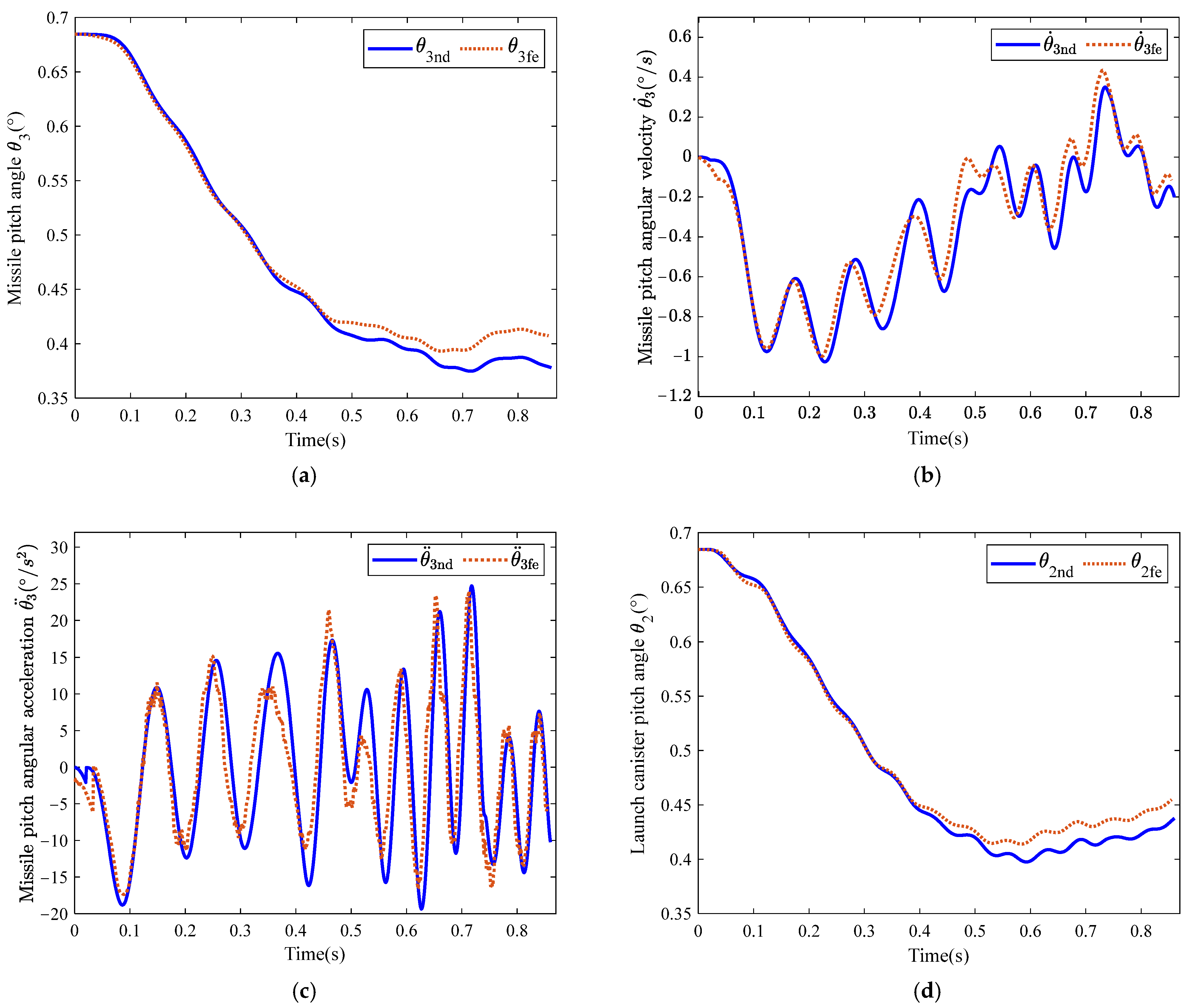
4.1. Verification of the 6-DOF Multi-Rigid-Body Launch Dynamic Model

In order to verify the effectiveness of the proposed missile launch dynamics controller, the multi-rigid-body dynamic numerical model of the VMLS, based on numerical calculation software, is established. Meanwhile, the launch dynamics simulation results from the finite element model of the launch system are compared with the mathematical model calculation results to verify the correctness of the 6-DOF multi-rigid-body launch dynamic model (this finite element model is an abstract model that sufficiently reflects the URVL dynamic process and is not associated with any actual equipment). The sample time is set to 0.001s, and the simulation time is set to 0.86 s. The simulation process lasts until the missile is completely detached from the launch canister, and the model parameters are shown in

Table 1. Launch dynamic model parameters.

Model Parameter	Value	Model Parameter	Value
m1/kg	38,000	${\overline{y}}_2$/m	−6.065
m2/kg	14,950	D/m	2
m3/kg	42,470	z1/m	5.324
J1/kg·m2	1.42 × 106	z2/m	1.634
J2/kg·m2	2.98 × 105	z3/m	−2.826
J3/kg·m2	1.11 × 106	z4/m	−7.226
kl/N·m−3	1.6 × 107	μ	0.16
ca/N·m−1·s−1	10	βe/Pa	7 × 108
ks1/N·m−1	6 × 107	Ps/Pa	3.5 × 107
cs1/N·m−1·s−1	6 × 105	Pr/Pa	0
ks2/N·m−1	6 × 107	A1/m2	0.0283
cs2/N·m−1·s−1	6 × 105	A2/m2	0.017
${\overline{x}}_1$/m	−10.580	V01/m2	0.051
${\overline{y}}_1$/m	0.591	V02/m2	0.0119
${\overline{x}}_2$/m	1.198	kq	0.7

.

Figure 3 compares the simulation results of the finite element model and the mathematical model for the attitude change. The subscript nd in Figure 3 represents the case without lumped disturbances, which is calculated by the mathematical model; the subscript fe represents the case without lumped disturbances, which is calculated by the finite element model. The max deviation error between the mathematical model and the finite element model for the result of missile body angle is 7.24%, and the trends of the results for the missile angular velocity, missile angular acceleration, and launch canister angle are also the same. Therefore, the proposed mathematical model is able to reflect the URVL dynamic process relatively accurately. In the case without the lumped disturbances, the VMLS is supported on rigid ground, and the missile is turned by an angle of 0.38° relative to the global coordinate system in the counterclockwise direction when it is detached from the launch canister, with an angular velocity of −0.2°/s. The changes in the angle and angular velocity of the missile are relatively small, and the launching process is stable.

4.2. Launch Dynamics in Uncontrolled State with Lumped Disturbances

To simulate the real launch response, we fit the differences between the simulation results of the angular acceleration of the missile, the lateral acceleration, and the angular acceleration of the launch canister calculated by the finite element method, taking into account the disturbance factors such as the deformation of the launch site, the flexibility of the system structure, and the results of the mathematical model calculated without considering the total interference by means of trigonometric combinations, and we obtain the mathematical forms of the three lumped disturbances, which are d₁, d₂, and d₃. In this way, we are able to analyze the degree of influence of the lumped disturbances from the point of view of amplitude and frequency. The amplitude of d₄ is taken as about 10% of the peak value of the simulation result of ${\dot{X}}_7$ in its corresponding state-space equation, and its frequency is also taken with reference to the simulation result of ${\dot{X}}_7$. The lumped disturbances $d_1$~$d_4$ are also introduced, denoted as

$$\left\{\begin{array}{l}{d}_1=1.8\times {10}^{-3}\times \sin 30\pi t\\ +0.09\times \sin 0.5\pi t\times e^{-10t}\\ d_2=0.0235\times \sin 10\pi t\\ d_3=0.23\times \sin 5\pi t\times e^{-10t}\\ +0.115\times \sin 0.5\pi t\times e^{-10t}\\ d_4=8\times {10}^6\times \sin 20\pi t\end{array}\right.,$$

(81)

According to the results in Figure 4, affected by the lumped disturbances (mainly caused by the deformation of the launching site presented in $d_3$), the missile is turned by an angle of 3° in the counterclockwise direction relative to the global coordinate system when it is detached from the launch canister, with an angular velocity of 6.23°/s. The evaluation index of launching site adaptability, as mentioned in Reference [3], is that the absolute values of the pitch angle and angular velocity of the missile do not exceed 5° and 5°/s, respectively, when the missile is detached from the launch canister. Under uncontrolled launch conditions, the angular velocity of the missile exiting the launcher exceeds the safety threshold, which is difficult to accept for actual launch missions. Therefore, the missile’s attitude needs to be controlled during the launch process to ensure that the missile’s angle and angular velocity remain within the safety threshold.

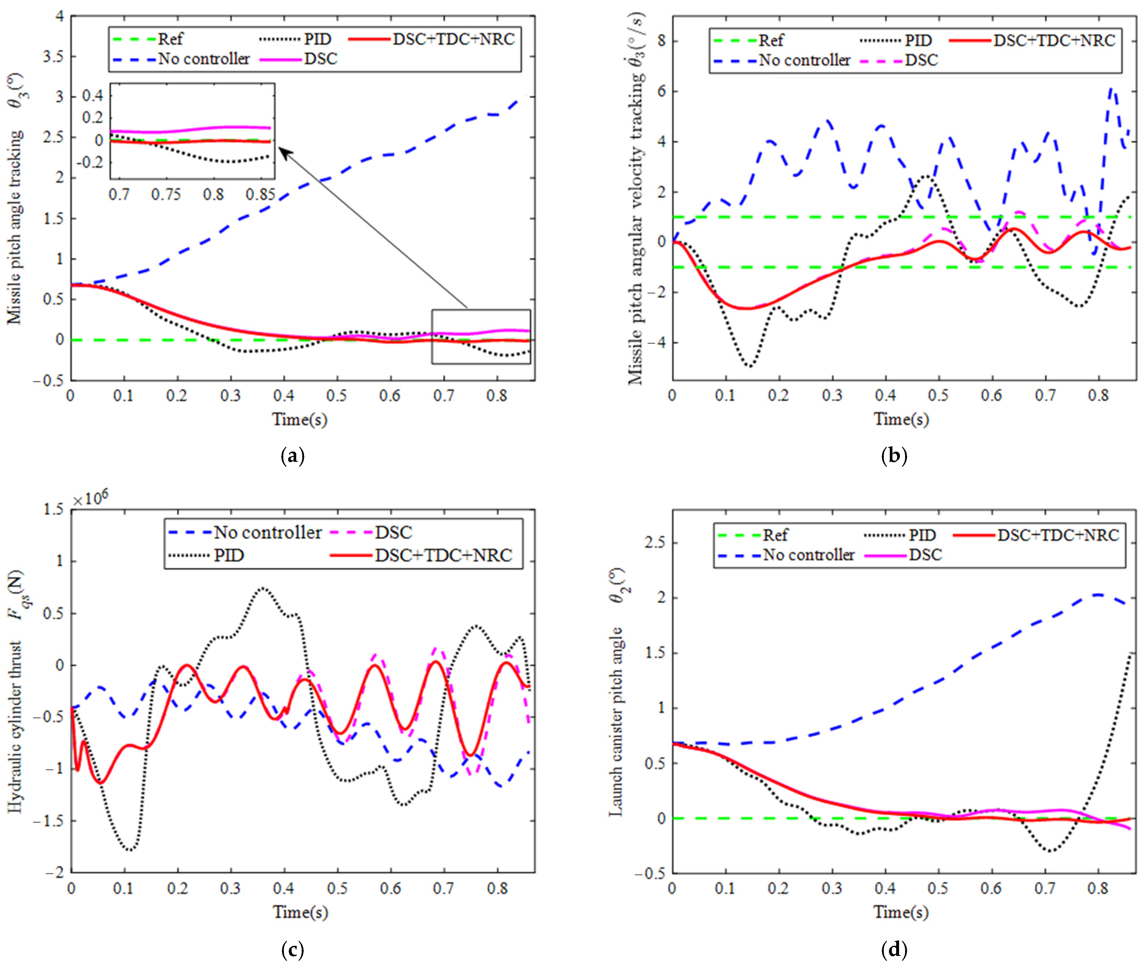
4.3. Launch Dynamics in Controlled State with Lumped Disturbances

In this paper, the control objective of the cold launch response of the missile is to keep the missile in vertical motion as much as possible with respect to the global coordinate system. The simulation of the missile attitude control during the vertical launching process is carried out based on PID, DSC, and DSC + TDC + NRC controllers, respectively. By collecting and calculating the pitch angle error, angle error derivative, and angle error integral of the projectile, the PID controller is designed employing commonly used PID principles and implemented through parameter tuning. The parameters of the PID controller are set to $k_P=50$, $k_I=0.001$, and $k_D=6$. The control parameters of the DSC controller are set to $k_1=10$, $k_2=1.1\times {10}^4$, $k_3=20$, $k_4=450$, $k_5=25$, $k_6=4$, and $k_7=100$. The time constants are set to ${\tau }_1=0.001$, ${\tau }_2=0.001$, ${\tau }_3=0.001$, ${\tau }_4=0.001$, ${\tau }_5=0.02$, and ${\tau }_6=0.001$. The parameters of nonlinear filters are set to ${\eta }_1=2$, ${\eta }_2=0.5$, ${\eta }_3=2$, ${\eta }_4=0.5$, ${\eta }_5=10$, ${\eta }_6={10}^5$, and $\sigma =1000/(1+t^2)$. The step size for time delay estimation $L$ is set to be consistent with the sample time, which is 0.001 s. The other parameters of the TDC are set to ${\overline{E}}_1=0.006$, ${\overline{E}}_2=2\times {10}^{-4}$, ${\overline{E}}_3=6\times {10}^5$, and ${\overline{E}}_4=3\times {10}^{-5}$. The parameters of NRC are set to ${\Delta }_1=600$, ${\Delta }_2=120$, ${\Delta }_3=5$, and ${\Delta }_4=4\times {10}^6$. During the parameter debugging process for each controller, we calculated the relevant indicator data (such as root mean square error (RMSE), maximum error of angle tracking, and angular velocity) from 0.6 s to 0.86 s, as shown in

Table 2. Comparison of control effects of three controllers.

Index $(\mathit{t}\ge 0.6 \mathbf{s}$)	No Control	PID	DSC	DSC + TDC + NRC
$e_{1\mathrm{sm}}$	3.1175	0.1121	0.0839	0.0145
$e_{1\max }$	3.0233	0.1887	0.12	0.0271
${\dot{\theta }}_{3\mathrm{sm}}$	3.3015	1.5397	0.6092	0.3346
${\dot{\theta }}_{3\max }$	6.2344	2.5472	1.2024	0.3030

, and increased the control parameters through the evaluation of each indicator. Until the control gain increases to the point where the curve oscillates and the index deteriorates, we choose the control parameter with the beter index as the control parameter for comparing the control effect.

Figure 5 shows the angle tracking error of the missile, the angular velocity of the missile, the hydraulic actuator force, and the launch canister angle under the three controllers, respectively. It can be seen that the control performance of the PID controller is poor for dynamical processes with short-time highly nonlinear and strongly perturbed dynamics. The DSC controller with the backstepping design is able to ensure fast convergence of the tracking by tuning the control gain of the linear feedback terms in the virtual control inputs of each order large enough to stabilize the system. However, the stabilizing effect of linear feedback terms on the lumped disturbances is still limited, and the use of the DSC controller only is insufficient to ensure the safety of the launch in a realistic random unknown launch environment. The DSC + TDC + NRC controller compensates for the model uncertainties in the system through the estimation of the lumped disturbances and further attenuates the TDE error by utilizing the nonlinear robust terms, which keeps the maximum angle error at the moment of the missile’s exit from the launch canister within 0.05° and the maximum angular velocity within 0.5°/s. In addition, the proof of the DSC + TDC + NRC controller theoretically guarantees the semi-global asymptotic convergence of the system error.

To further quantitatively illustrate the performance of the proposed control approach, the root mean square error (RMSE) and maximum error of the angle tracking and angular velocity are collected in Table 2 (taking the data from 0.6 s to 0.86 s). It can be found that compared with the PID controller, the RMSE of the angle tracking and angular velocity of the proposed controller DSC + TDC + NRC is reduced by 7.7 times and 4.6 times, respectively. Compared with the DSC controller, the RMSE of angle tracking and angular velocity of the proposed controller DSC + TDC + NRC is reduced by 5.8 times and 1.8 times, respectively. In summary, the proposed controller DSC + TDC + NRC obtained the most satisfactory control performance for missile attitude, which can improve launch safety and the adaptability of the launch system to the site.

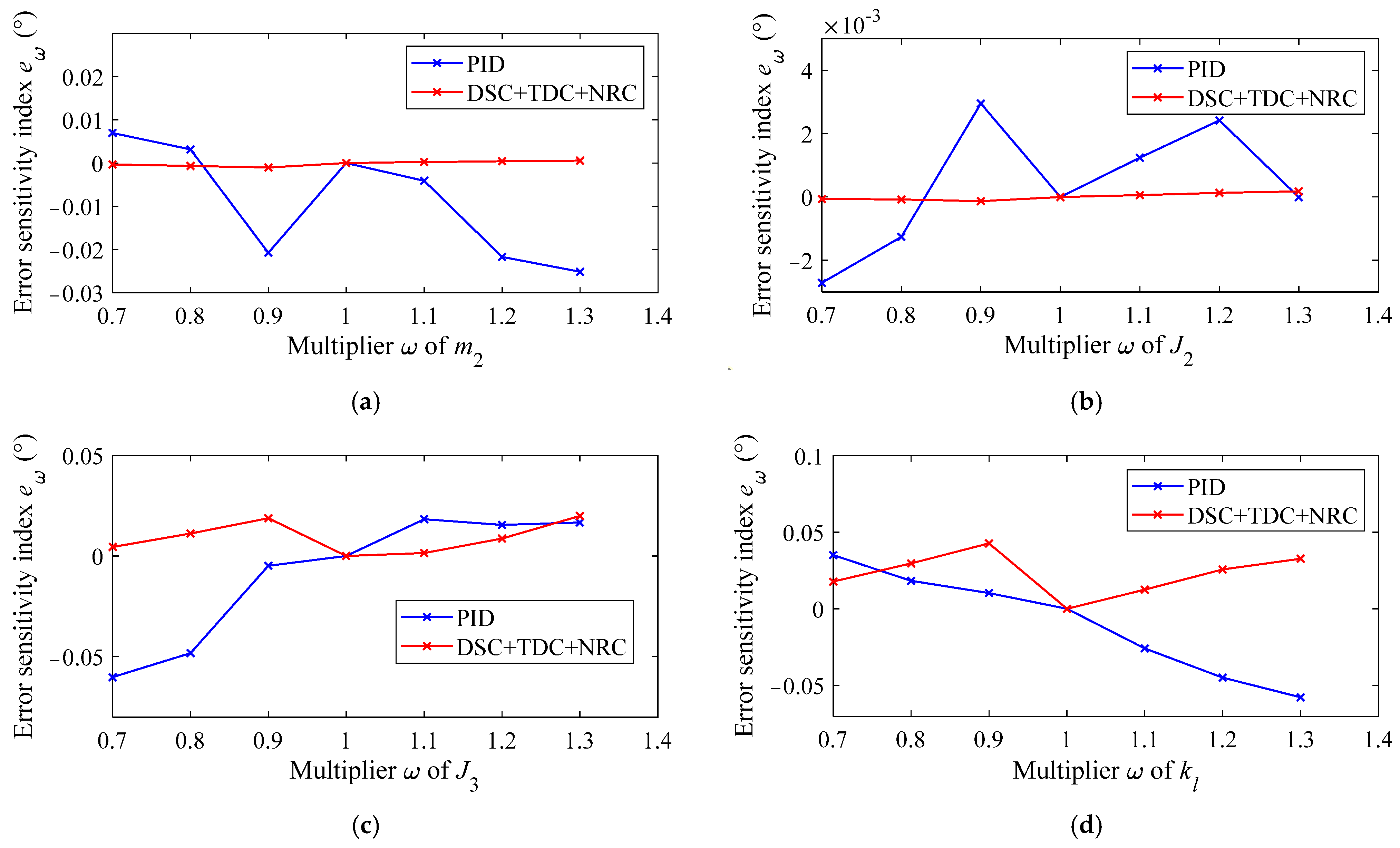
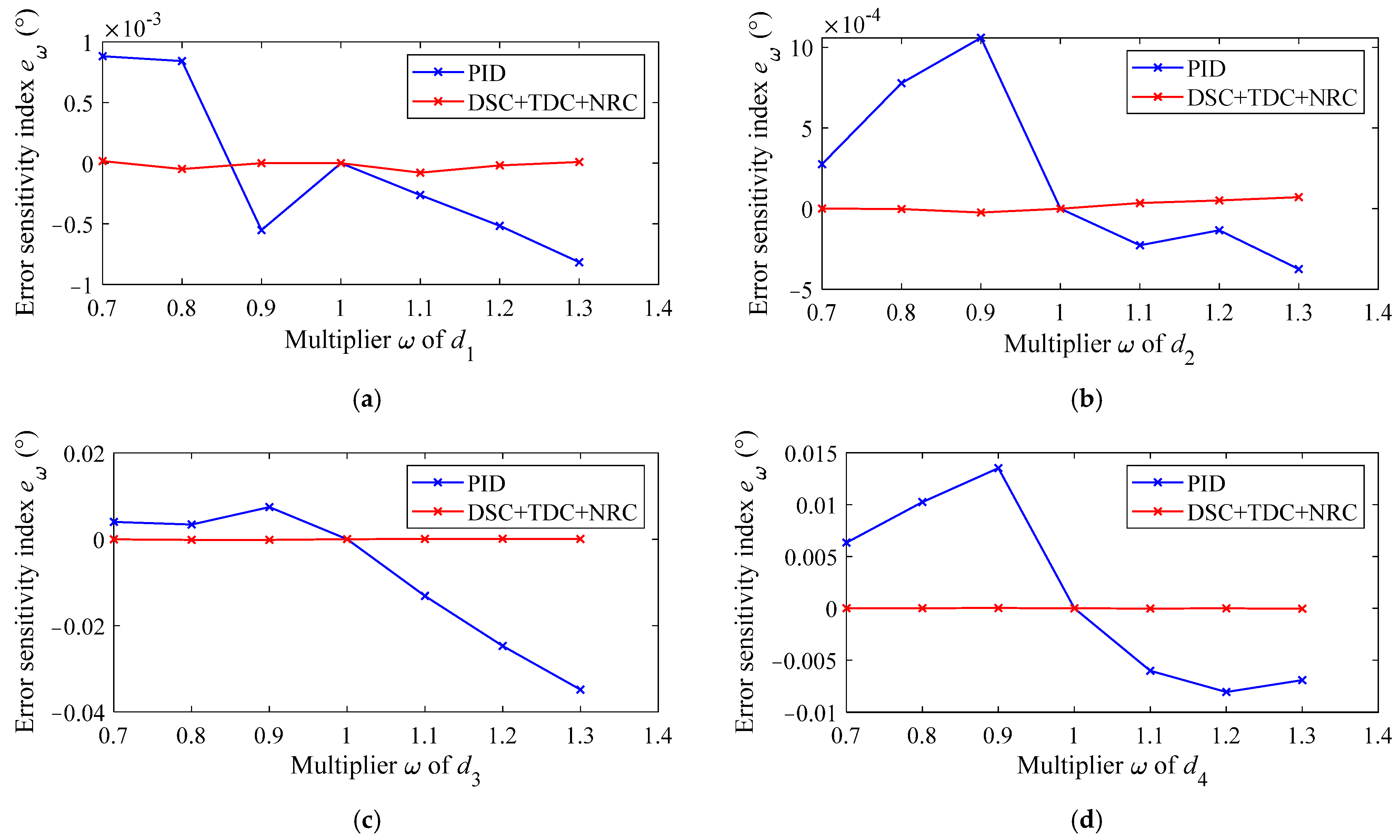
4.4. Error Sensitivity Analysis of System Parameters and Lumped Disturbance Terms

In order to further validate the adaptability of the proposed control method for launch response control in a real random unknown launch environment, this paper conducts a sensitivity analysis of the launch response control for four key model parameters, including the mass of the launch canister $m_2$, the moment of inertia of the launch canister $J_2$, the moment of inertia of the missile $J_3$ and the linear radial stiffness of the adapters $k_l$, and the four lumped disturbance terms ($d_1$, $d_2$, $d_3$, and $d_4$). All four model parameters and the four lumped disturbance terms are varied by plus or minus 30% from their current values, and the results of the error sensitivity analysis are compared between the PID and DSC + TDC + NRC controllers for launch response control, which are as shown in Figure 6 and Figure 7. We define an error sensitivity index $e_{\omega }=e_{1sm}(\omega )-e_{1sm}(1)$ to measure the degree of influence of the model parameters and the lumped disturbance terms on the control performance of two controllers, in which $\omega$ is a multiplier ($\omega$ can take values of 0.7, 0.8, 0.9, 1, 1.1, 1.2, and 1.3), $e_{1sm}(\omega )$ is the root mean square error (RMSE) under the influence of multiplier $\omega$, and $e_{1sm}(1)$ is the root mean square error (RMSE) under the influence of multiplier $\omega =1$. From the comparison results, it is clear that $e_{\omega }$ is more sensitive to the changes in the four parameters and the four lumped disturbance terms when using the PID controller, whereas the DSC + TDC + NRC controller is able to maintain a good control effect in the case of changes caused by the change in the bearing capacity of the launching site and the change in the model structural parameters due to its anti-disturbance advantages. This means that the proposed control algorithm displays better adaptability and stability in the case of limited changes in the external launch environment and in the structural parameters of the system.

5. Conclusions

This paper proposes the idea of using the hydraulic actuator to actively regulate the missile attitude, which ensures the safety and stability of the launch process and the adaptability of the launch system to the site through the load transfer link from the hydraulic actuator, to the launch canister, to the adapters, and then to the missile. First, a 6-DOF dynamic model of the launch system, considering the dynamics of the hydraulic actuator, is established, and the seventh-order state-space equation is derived. Subsequently, based on the backstepping design philosophy, the design of the main controller is carried out using the DSC method, which realizes the stabilization of the matched and mismatched terms. In order to suppress the effects of these complex factors, such as modeling errors, dynamic deformation of launching site, flexibility of vehicle structure, and launch vibration, on the launch response control performance, inspired by the time-delay estimation technique, the matched and mismatched lumped disturbances combining the above nonlinear uncertainties in the state-space equation are estimated, and the estimated values are introduced into the DSC controller for disturbance attenuation. The mathematical model calculation results are compared with the results from the finite element model, and the correctness of the developed launch dynamic model is verified. In addition, by comparing the simulation results of the launch response obtained by the three control methods, PID, DSC, and DSC + TDC + NRC, and further comparing the error sensitivity under the variation of the model parameters and the lumped disturbance terms in the two methods, PID and DSC + TDC + NRC, the control effectiveness of DSC + TDC + NRC in the short-time highly nonlinear and strongly perturbed dynamics process is verified, which provides a new way of thinking regarding the reliable launching of the VMLS in the real random unknown launching environment.

However, the problems addressed in this paper still require further research to provide the engineering means to support reliable launching in random unknown launch environments. Despite the initial bold exploration of missile attitude control carried out in this paper via a hydraulic cylinder, the proposed control strategy is still potentially immature and lacks the comparisons of control effectiveness with commonly used methods, such as command filtered control, tracking differentiators, and disturbance observers. The performance of the control algorithm in the presence of measurement noise also remains uninvestigated. In addition, the dynamic response of the launching site (especially the unpaved site) under the short-time strong impact condition remains a field rarely studied by scholars, which is of great significance for the demonstration and evaluation of launching safety and launching site adaptability. Furthermore, the validation of the control methods of launch response by principle-based test prototypes is an inevitable method of technical engineering. However, safe and realistic experimental means for such a complex system are still difficult to develop at present. The authors will further explore these problems in subsequent research.

References

1. Cheng, H.; Qian, Z.; Zhao, Y.; Li, B. Study on the load to ground on missile erection process. Ordn. Ind. Autom. 2011, 30, 1–3. [Google Scholar]
2. Zhou, X.; Ma, D.; Hu, J.; Zhong, J. Research on dynamic response of launching site for missile unsupported random launch. Acta Armamentarii 2014, 35, 1595–1603. [Google Scholar]
3. Zhang, Z.; Ma, D.; Zhong, J.; Gao, Y.; Wang, X. Research on adaptability of a cold launching system of missile to launching site. Acta Armamentarii 2020, 41, 280–290. [Google Scholar]
4. Zhang, T.; Liu, X.; Zheng, B. Rigid-flexible coupling dynamic analysis during launching based on component model synthesis. Missiles Space Veh. 2009, 1, 51–54. [Google Scholar]
5. Gao, X.; Bi, S.; Chen, Z. The Simulation study on multi-body launching dynamics for a vehicular missile launcher. J. Project. Rock. Miss. Guid. 2010, 30, 60–62. [Google Scholar]
6. Rui, X. Launch dynamics of multibody systems and its applications. Str. St. CAE 2011, 13, 76–82. [Google Scholar]
7. Işık, C.; Ider, S.; Acar, B. Modeling and verification of a missile launcher system. Proc. Inst. Mech. Eng. 2013, 228, 100–107. [Google Scholar] [CrossRef]
8. Yang, C.; Ma, D.; Wang, X. Sensitivity analysis of factors affecting launching-site dynamic response of missile with unsupported random launch. J. Ball. 2016, 28, 87–92. [Google Scholar]
9. Cheng, H.; Zhang, Y.; Li, B.; Zhan, J. Research on the bearing capacity of unsupported random launching site. In Proceedings of the 2011 International Conference on Advanced Materials and Engineering Materials (ICAMEM), Shenyang, China, 22–24 January 2012. [Google Scholar]
10. Zhang, Z.; Ma, D.; Ren, J.; He, Q.; Zhu, Z. Dynamic response of cold launching equipment to prepared launching site subjected to loading. Ordn. Ind. Autom. 2015, 36, 279–286. [Google Scholar]
11. Zhou, X.; Wang, H.; Ma, D.; Gao, Y.; Ren, J. Study on unsupported launching site quasi-static response during missile standby phase. J. Ball. 2015, 27, 91–96. [Google Scholar]
12. Sun, C.; Ma, D.; Ren, J. Study on vertical launching response characteristics of cold launch platform. J. Nanjing Univ. Sci. Techn. 2015, 39, 516–522+555. [Google Scholar]
13. Pan, Q.; Liang, G.; Lyu, Y.; Qi, Z.; Liu, H. Fast simulation on rigid multibody dynamics for vehicular cold launch systems. J. Beijing Univ. Aeronaut. Astronaut. 2017, 43, 71–78. [Google Scholar]
14. Wang, X.; Rui, X.; Yang, F.; Zhou, Q. Launch dynamics modeling and simulation of vehicular missile system. J. Guid. Control Dyn. 2018, 41, 1370–1379. [Google Scholar] [CrossRef]
15. Zhou, F.; Li, D.; Zhou, S.; Jiang, R. Semianalytical model for dynamic analysis of missile vertical cold launch. J. Spacecr. Rockets 2022, 59, 1966–1986. [Google Scholar] [CrossRef]
16. Pan, Q.; Liang, G.; Lyu, Y.; Qi, Z.; Wang, X. Modeling and simulation of rigid-flexible coupling dynamics of vehicular cold launch system. Ordn. Ind. Autom. 2017, 38, 2386–2394. [Google Scholar]
17. Swaroop, D.; Hedrick, J.K.; Yip, P.P.; Gerdes, J.C. Dynamic surface control for a class of nonlinear systems. IEEE Trans. Automat. Contr. 2000, 45, 1893–1899. [Google Scholar] [CrossRef]
18. Jing, C.; Xu, H.; Jiang, J. Dynamic surface disturbance rejection control for electro-hydraulic load simulator. Mech. Syst. Signal Process. 2019, 134, 106293. [Google Scholar] [CrossRef]
19. Wang, Y.; Zhao, J.; Ding, H.; Zhang, H. Dynamic surface control based on high-gain disturbance observer for electro-hydraulic systems with position/velocity constraints. Proc. Inst. Mech. Eng. C J. Mech. Eng. Sci. 2021, 235, 3485–3494. [Google Scholar] [CrossRef]
20. Sa, Y.; Zhu, Z.; Tang, Y.; Li, X.; Shen, G. Adaptive dynamic surface control using nonlinear disturbance observers for position tracking of electro-hydraulic servo systems. Proc. Inst. Mech. Eng. I J. Syst. Control Eng. 2022, 236, 634–653. [Google Scholar] [CrossRef]
21. Zhang, X.; Shi, G. Dual extended state observer-based adaptive dynamic surface control for a hydraulic manipulator with actuator dynamics. Mech. Mach. Theory 2022, 169, 104647. [Google Scholar] [CrossRef]
22. Gao, Q.; Wei, X.; Li, D.; Ji, Y.; Chao, J. Tracking control for a quadrotor via dynamic surface control and adaptive dynamic programming. Int. J. Control Autom. Syst. 2022, 20, 349–363. [Google Scholar] [CrossRef]
23. Yang, X.; Ge, Y.; Deng, W.; Yao, J. Precision motion control for electro-hydraulic axis systems under unknown time-variant parameters and disturbances. Chin. J. Aeronaut. 2024, 37, 463–471. [Google Scholar] [CrossRef]
24. Chen, W.; Yang, J.; Guo, L.; Li, S. Disturbance-observer-based control and related methods—An overview. IEEE Trans. Ind. Electron. 2016, 63, 1083–1095. [Google Scholar] [CrossRef]
25. Sun, C.; Fang, J.; Wei, J.; Li, M. Nonlinear motion control of a hydraulic press based on an extended disturbance observer. IEEE Access 2018, 6, 18502–18510. [Google Scholar] [CrossRef]
26. Liu, J.; Gai, W.; Zhang, J.; Li, Y. Nonlinear adaptive backstepping with ESO for the quadrotor trajectory tracking control in the multiple disturbances. Int. J. Control Autom. Syst. 2019, 17, 2754–2768. [Google Scholar] [CrossRef]
27. Deng, W.; Yao, J.; Wang, Y.; Yang, X.; Chen, J. Output feedback backstepping control of hydraulic actuators with valve dynamics compensation. Mech. Syst. Signal Process. 2021, 158, 107769. [Google Scholar] [CrossRef]
28. Shao, X.; Xu, L.; Zhang, W. Quantized control capable of appointed-time performances for quadrotor attitude tracking: Experimental validation. IEEE Trans. Ind. Electron. 2021, 69, 5100–5110. [Google Scholar] [CrossRef]
29. Yang, G.; Yao, J.; Ullah, N. Neuroadaptive control of saturated nonlinear systems with disturbance compensation. ISA Trans. 2022, 122, 49–62. [Google Scholar] [CrossRef]
30. Hsia, T.S. A new technique for robust control of servo systems. IEEE Trans. Ind. Electron. 1989, 36, 1–7. [Google Scholar] [CrossRef]
31. Youcef-Toumi, K.; Ito, O. A time delay controller for systems with unknown dynamics. J. Dyn. Syst. Meas. Control 1990, 112, 133–142. [Google Scholar] [CrossRef]
32. Lee, S.U.; Chang, P.H. Control of a heavy-duty robotic excavator using time delay control with integral sliding surface. Control Eng. Pract. 2002, 10, 697–711. [Google Scholar] [CrossRef]
33. Jin, M.; Lee, J.; Ahn, K.K. Continuous nonsingular terminal sliding-mode control of shape memory alloy actuators using time delay estimation. IEEE/ASME Trans. Mech. 2014, 20, 899–909. [Google Scholar] [CrossRef]
34. Kim, J.; Joe, H.; Yu, S.; Lee, J.; Kim, M. Time-delay controller design for position control of autonomous underwater vehicle under disturbances. IEEE Trans. Ind. Electron. 2015, 63, 1052–1061. [Google Scholar] [CrossRef]
35. Lee, J.; Chang, P.H.; Jin, M. Adaptive integral sliding mode control with time-delay estimation for robot manipulators. IEEE Trans. Ind. Electron. 2017, 64, 6796–6804. [Google Scholar] [CrossRef]
36. Vo, C.P.; Dao, H.V.; Ahn, K.K. Actuator fault-tolerant control for an electro-hydraulic actuator using time delay estimation and feedback linearization. IEEE Access 2021, 9, 107111–107123. [Google Scholar]
37. Wang, C. Research on Launching Attitude of Ballistic Missile Unsupported Random Cold Launching. Master’s Thesis, Harbin Institute of Technology, Harbin, China, 30 June 2019. [Google Scholar]
Figure 1. Multi-rigid-body dynamic model of a vehicle-mounted missile cold launch system.
Actuators 14 00142 g001
Figure 2. The geometric relationship between missile, adapters, and launch canister: (a) initial state; (b) launch process.
Actuators 14 00142 g002
Figure 3. Comparison of the simulation results of attitude change from the finite element model and the mathematical model: (a) curve of missile angle; (b) curve of missile angular velocity; (c) curve of missile angular acceleration; (d) curve of launch canister angle.
Actuators 14 00142 g003
Figure 4. Attitude changes of missile and launcher in uncontrolled state, with and without the lumped disturbances: (a) curve of missile angle; (b) curve of missile angular velocity; (c) curve of missile angular acceleration; (d) curve of launch canister angle.
Actuators 14 00142 g004
Figure 5. Comparison of the control effect of the three controllers: (a) comparison of missile angle tracking performance; (b) comparison of missile angular velocity; (c) hydraulic actuator thrust of three controllers; (d) comparison of launch canister angle.
Actuators 14 00142 g005
Figure 6. Comparison of the control effect under the variation of four key model parameters: (a) comparison under the variation of m 2 ; (b) comparison under the variation of J 2 ; (c) comparison under the variation of J 3 ; (d) comparison under the variation of k l .
Actuators 14 00142 g006
Figure 7. Comparison of the control effect under the variation of four lumped disturbance terms: (a) comparison under the variation of d 1 ; (b) comparison under the variation of d 2 ; (c) comparison under the variation of d 3 ; (d) comparison under the variation of d 4 .
Actuators 14 00142 g007