
Quantitative Biofacies Analysis to Identify Relationships and Refine Controls on Paleosol Development, Prince Creek Formation, North Slope Alaska, USA

Abstract
:1. Introduction
2. Materials and Methods
3. Results
3.1. Hierarchical Agglomerative Cluster Analysis (HCA)
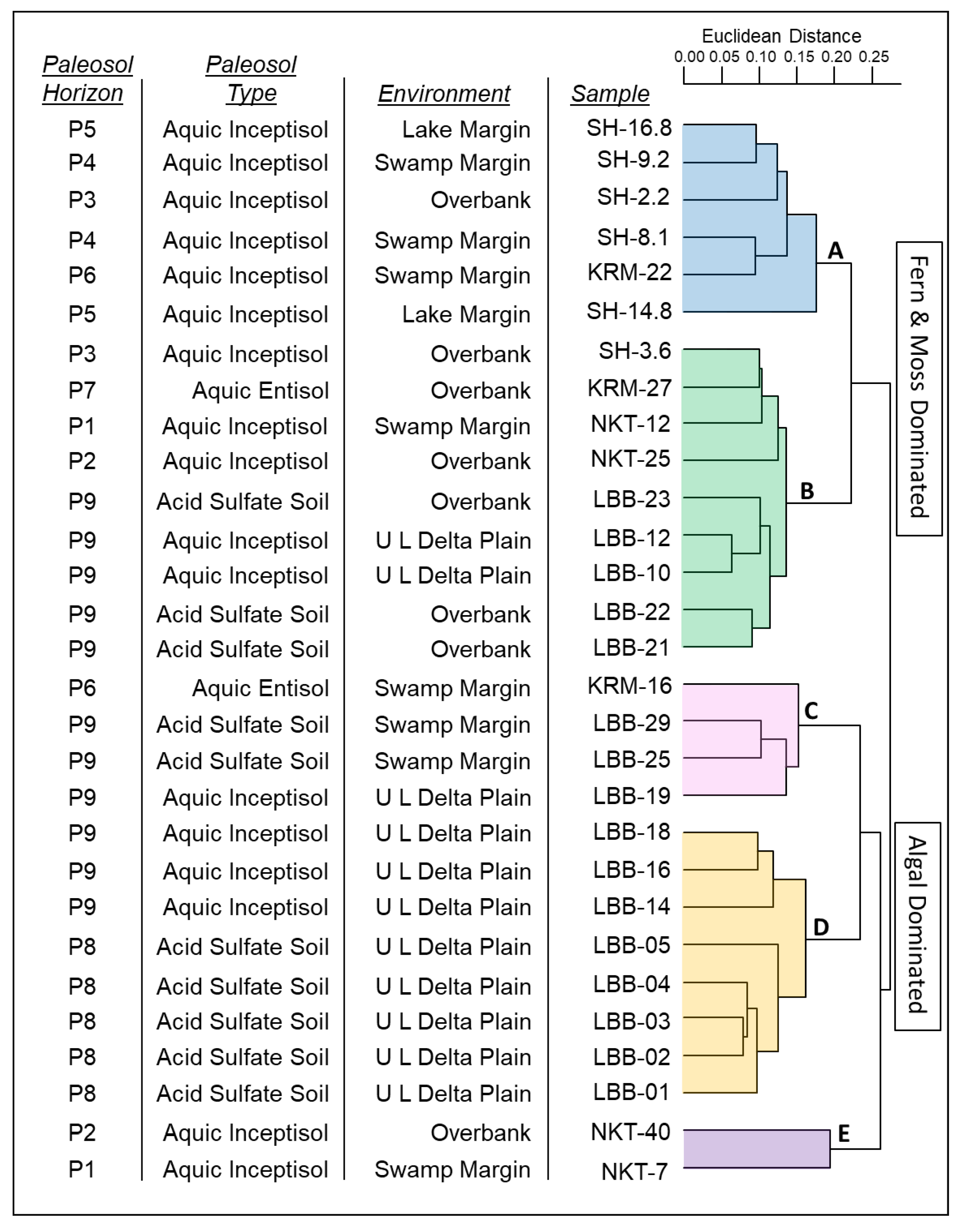
- Five clusters, referred to as biofacies A–E are interpreted in the cluster dendrogram (see Figure 4).
- A significant branch point at a Euclidean distance of 0.25 separates biofacies A and B from biofacies C, D, and E (Figure 4). This branch reflects a major break in biotic composition, from the fern and moss dominated samples of biofacies A and B to the brackish and freshwater algae dominated assemblages of biofacies C, D, and E.
- In general, clusters tend to differentiate samples among the localities and the depositional environments from which they were collected, although overlap exists. The clusters do not cleanly segregate samples of different paleosol types or from different paleosol horizons, although loose groupings are observed (see Figure 4).
- Biofacies A mainly comprises swamp and lake margin samples from the P3 through P6 paleosol horizons of the Sentinel Hill and Kikiakrorak River Mouth localities. Fern and moss spores dominate, especially Psilatriletes, and comprise 56% of the biofacies. Brackish and freshwater algae, including Sigmapollis, are common and comprise 19% of the total counts in the biofacies (see Figure 4 and Table 2).
- Biofacies B mainly contains samples from overbank facies of the P2, P3, P7, and P9 paleosol horizons from all four localities. Similar to biofacies A, biofacies B is also dominated by fern and moss spores (43%) and algae (25%). Unlike biofacies A, Psilatriletes is rarely encountered. Instead, the spore Laevigatosporites is the most abundant genus (15%) (see Figure 4 and Table 2).
- Biofacies C mainly contains samples from swamp margins from the P6 and P9 paleosols of the Liscomb Bonebed and Kikiakrorak River Mouth localities. Brackish and freshwater algae (39%) and exotic pollen (26%) are dominant. Diagnostic taxa include Sigmapollis and the pollen genus Aquilapollenites (see Figure 4 and Table 2).
- Biofacies D is characterized by samples from the undifferentiated lower delta plain from the P8 and P9 paleosols of the Liscomb Bonebed. Biofacies D contains a high abundance of brackish and freshwater algae (50%) and fern and moss (22%) genera. Sigmapollis is dominant, composing nearly 40% of the biofacies (see Figure 4 and Table 2).
- Biofacies E comprises two samples from overbank and swamp margin deposits of the P1 and P2 paleosols from the North Kikak-Tegoseak locality. It contains the highest proportion of algae genera (70%) observed. Unlike the other algae dominated samples from biofacies C and D, in biofacies E Botryococcus algae, not Sigmapollis, is diagnostic (see Figure 4 and Table 2).
3.2. Detrended Correspondence Analysis
- Coding the samples by biofacies membership reveals that the DCA results largely support the results of the cluster analysis.
- The major segregation between fern and moss dominated biofacies (A and B) and algae dominated biofacies (C, D, and E) is clearly observable (see Figure 5A). Algae dominated samples have low axis 2 scores, while fern and moss dominated samples have intermediate to high axis 2 scores. The DCA scores of select algae genera (Sigmapollis and Botryococcus) and fern and moss genera (Psilatriletes, Aquilapollenites, Deltoidospora, and Laevigatosporites), as well as the average scores of all taxa from these two respective ecological groups, support the separation of algae from fern and moss dominated assemblages.

- Coding the samples by paleosol horizon reveals no easily generalized temporal trend, although samples from each individual horizon tend to plot closely in space (see Figure 5C). Samples from P4, P5, P6, P7, P8, and P9 have low to intermediate axis 1 scores, samples from P1 and P3 have intermediate axis 1 scores, and samples from P2 have the highest axis 1 scores. The P1, P2, P8, and P9 samples separate from the P3, P4, P5, P6, and P7 samples along axis 2.
- When samples are coded by paleosol taxonomy, a weak separation is observed between samples from acid sulfate soils (horizons P8 and P9 from the Liscomb Bonebed) and the aquic entisols and inceptisols that characterize all other samples (see Figure 5D).
- Coding samples by depositional environment reveals that swamp and lake margin samples tend to have low and intermediate axis 1 scores and intermediate to high axis 2 scores; the undifferentiated lower delta plain samples tend to have low and intermediate axis 1 and low axis 2 scores; overbank samples display intermediate to high axis 1 scores and intermediate axis 2 scores (see Figure 5E).
- Swamp margin, lake margin, and overbank facies are dominated by fern and moss genera, which comprise nearly 40% of each environment’s biota (see Table 3). Swamp and lake margin samples share many common and abundant genera, including Psilatriletes and Sigmapollis. Variation in the abundances of the lowland tree/shrub Taxodiaceaepollenites and the algae Pediastrum differentiate the swamp and lake margin (see Table 4). Plotting the scores of taxa within DCA space corroborates these compositional trends. The average score of fern and moss taxa plots closely to swamp and lake margin samples and nearby to overbank samples, indicating they are common elements of these environments.

| Locality | Palynomorph Abundance | Generic Abundance | ||||
|---|---|---|---|---|---|---|
| Swamp Margin | Ferns & Mosses | 39 | Psilatriletes (F&M) | 16 | Taxodiaceaepollenites (LTS) | 4 |
| Algae | 29 | Sigmapollis (A) | 16 | Leiospheres (A) | 3 | |
| Exotic Projectate | 16 | Aquilapollenites (EP) | 13 | Osmundacidites (F&M) | 3 | |
| Lowland Tree/Shrub | 11 | Botryococcus (A) | 7 | Bisaccate pollen (HC) | 3 | |
| Hinterland Conifer | 3 | Laevigatosporites (F&M) | 6 | |||
| Deltoidospora (F&M) | 5 | |||||
| Lake Margin | Ferns & Mosses | 42 | Taxodiaceaepollenites (LTS) | 16 | Botryococcus (A) | 6 |
| Algae | 29 | Psilatriletes (F&M) | 14 | Osmundacidites (F&M) | 5 | |
| Lowland Tree/Shrub | 20 | Sigmapollis (A) | 9 | Leiospheres (A) | 4 | |
| Exotic Projectate | 4 | Pediastrum (A) | 9 | |||
| Hinterland Conifer | 3 | Laevigatosporites (F&M) | 7 | |||
| Deltoidospora (F&M) | 6 | |||||
| Overbank | Ferns & Mosses | 38 | Sigmapollis (A) | 15 | Deltoidospora (F&M) | 5 |
| Algae | 31 | Laevigatosporites (F&M) | 12 | Osmundacidites (F&M) | 5 | |
| Lowland Tree/Shrub | 11 | Bisaccate pollen (HC) | 8 | Aquilapollenites (EP) | 4 | |
| Hinterland Conifer | 9 | Taxodiaceaepollenites (LTS) | 6 | Lycopodiumsporites (F&M) | 4 | |
| Exotic Projectate | 5 | Botryococcus (A) | 6 | Psilatriletes (F&M) | 3 | |
| Prasinophyceae (A) | 5 | Stereisporites (F&M) | 3 | |||
| Undiff. Lower Delta Plain | Algae | 44 | Sigmapollis (A) | 34 | Prasinophyceae (A) | 3 |
| Ferns & Mosses | 28 | Laevigatosporites (F&M) | 11 | Leiospheres (A) | 3 | |
| Lowland Tree/Shrub | 14 | Taxodiaceaepollenites (LTS) | 5 | Psilatriletes (F&M) | 3 | |
| Hinterland Conifer | 5 | Osmundacidites (F&M) | 4 | Bisaccate pollen (HC) | 2 | |
| Exotic Projectate | 3 | Porocolpopollenites (LTS) | 4 | Liliacidites (LTS) | 2 | |
| Stereisporites (F&M) | 3 | Deltoidospora (F&M) | 2 | |||
- Overbank samples are dominated by Sigmapollis and Laevigatosporites; Psilatriletes is rare. The overbank contains a higher proportion of hinterland conifer pollen, reworked dinocysts (~1%), and marine acritarchs and peridinoids (~1%) than the lake and swamp margins (see Table 4).
- The undifferentiated lower delta plain samples are dominated primarily by brackish and freshwater algae and secondarily by fern and moss genera. Sigmapollis is the most abundant taxon at 34% abundance (see Table 4). This environment contains the highest proportions of in situ and reworked marine elements (dinocysts and acritarchs) observed in the study (~3%), and these tend to plot close to undifferentiated lower delta plain samples in ordination space (see Figure 5E).
3.3. Analytic Rarefaction Analysis
- Rarefaction curves displaying richness at different sampling efforts are shown in Figure 6A–D.
- Biofacies B has a significantly higher taxonomic richness (61.4 taxa) as compared with other biofacies at the lowest common sampling effort (420 individuals). This is largely due to increased diversity of fern and moss and lowland tree and shrub taxa (see Table 5). Biofacies A, C, and D have lower and overlapping richness values (47.7, 45.1, and 49.1 taxa, respectively). Biofacies E has the lowest richness value (36.5 taxa) overall (see Figure 6A).
- The Liscomb Bonebed, North Kikak-Tegoseak, and Sentinel Hill localities display statistically indistinguishable richness values (66.3, 62.9, and 63.2 taxa, respectively) at the lowest common sampling effort (720 individuals). The Kikiakrorak River Mouth locality has significantly lower richness (57.2 taxa) (see Figure 6B and Table 6).
- The P9, P8, P7, P4, and P3 horizons have the highest and statistically overlapping richness values (40.8, 36.4, 42.1, 37.0, and 39.1 taxa, respectively) at the lowest common sampling effort (200 individuals). The P2 and P1 horizons have lower richness values (36.7 and 36.3 taxa, respectively), while the P6 and P5 display the lowest richness values (32.2 and 30.4 taxa, respectively) related to diminished diversity of algae, fern and moss, and lowland tree and shrub taxa (see Figure 6C and Table 7).

- Overbank environments have the richest assemblage (57.8 taxa) of any environment at the lowest common sampling effort (380 individuals). This is attributed to greater diversity of algae, fern and moss, hinterland conifer, lowland tree and shrub, and reworked marine taxa. The undifferentiated lower delta plain and swamp margin environments display overlapping and intermediate levels of richness (57.7 and 55.3 taxa, respectively); the lake margin has the lowest sampled richness (37.9 taxa) (see Figure 6D and Table 8).
4. Discussion
4.1. Environmental Controls on Biofacies Composition and Paleosol Development through Space
4.2. Environmental Controls on Biofacies Composition and Paleosol Development through Time
4.3. Future Research Directions
- How much biotic turnover is typical among depositional environments within a paleosol horizon? Does the level of between habitat variability change through time?
- Does each paleosol horizon contain a unique palynological/microbiotic signature, or does the biota tend to recur with only slight variations through time?
- What does any observed biotic variability tell us about the evolution of the coastal plain ecosystem and if/how physical environmental factors vary though time?
- How does the degree of biotic and environmental change observed compare to that in lower latitude Maastrichtian settings, where high frequency, seasonal changes may not be as evident?
- How similar are patterns of palynofacies variability and interpreted environmental controls in other marginal marine settings outside of the PCF?
4.4. Additional Uses of Quantiative Biofacies Analysis/Multivariate Statistical Tools
5. Conclusions
Supplementary Materials
Author Contributions
Funding
Data Availability Statement
Conflicts of Interest
References
- Davies, K.L. Duck-billed dinosaurs (Hadrosauridae: Ornithischia) from the North Slope of Alaska. J. Paleontol. 1983, 61, 198–200. [Google Scholar] [CrossRef]
- Parrish, M.J.; Parrish, J.T.; Hutchinson, J.H.; Spicer, R.A. Late Cretaceous vertebrate fossils from the North Slope of Alaska and implications for dinosaur ecology. PALAIOS 1987, 2, 377–389. [Google Scholar] [CrossRef]
- Spicer, R. Late Cretaceous floras and terrestrial environments of northern Alaska. In Alaska North Slope Geology; Taillur, I., Weimer, P., Eds.; Society of Economic Paleontologists and Mineralogists: Fullerton, CA, USA; The Alaska Geological Society: Anchorage, AK, USA, 1987; Volume 1, pp. 497–512. [Google Scholar]
- Parrish, J.T.; Spicer, R.A. Late Cretaceous terrestrial vegetation: A near-polar temperature curve. Geology 1988, 16, 22–25. [Google Scholar] [CrossRef]
- Spicer, R. Changing climate and biota. In The Cretaceous World; Skelton, P., Ed.; Cambridge University Press: Bakersfield, CA, USA; Cambridge, UK, 2003; pp. 85–162. [Google Scholar]
- Spicer, R.A.; Parrish, J. Late Cretaceous-early Tertiary paleoclimates of northern high latitudes: A quantitative view. Geol. Soc. Lond. 1990, 147, 329–341. [Google Scholar] [CrossRef]
- Rich, T.H.; Gangloff, R.A.; Hammer, W.H. Polar Dinosaurs. In Encyclopedia of Dinosaurs; Academic Press: San Diego, CA, USA, 1997; pp. 562–573. [Google Scholar]
- Fiorillo, A.R.; Gangloff, R.A. Theropod teeth from the Prince Creek Formation (Cretaceous) of northern Alaska, with speculations on arctic dinosaur paleoecology. J. Vertebr. Paleontol. 2000, 20, 675–682. [Google Scholar] [CrossRef]
- Rich, T.H.; Gangloff, R.A.; Hammer, W.H. Polar Dinosaurs. Science 2002, 295, 979–980. [Google Scholar] [CrossRef] [PubMed]
- Fiorillo, A.R.; Gangloff, R.A. Preliminary note on the taphonomic and paleoecologic setting of a Pachyrhinosaurus bonebed in northern Alaska. J. Vertebr. Paleontol. 2003, 23, 50A. [Google Scholar]
- Gangloff, R.A.; Fiorillo, A.R.; Norton, D.W. The first Pachycephalosaurine (Dinosauria) from the Paleo-Arctic and its paleogeographic implications. J. Paleontol. 2005, 79, 997–1001. [Google Scholar] [CrossRef]
- Fiorillo, A.R.; Tykoski, R.; Currie, P.; McCarthy, P.J.; Flaig, P.P. Description of two Troodon braincases from the Prince Creek Formation (Upper Cretaceous) North Slope, Alaska. J. Vertebr. Paleontol. 2009, 29, 178–187. [Google Scholar] [CrossRef]
- Fiorillo, A.R.; McCarthy, P.J.; Flaig, P.P.; Bandlen, E.; Norton, D.W.; Zippi, P.; Jacobs, L.; Gangloff, R.A. Paleontology and paleoenvironmental interpretation of the Kikak-Tegoseak Quarry (Prince Creek Formation: Late Cretaceous), northern Alaska: A multi-disciplinary study of a high-latitude ceratopsian dinosaur bonebed. In New Perspectives on Horned Dinosaurs; Ryan, M.J., Chinnery-Allgeier, B.J., Eberth, D.A., Eds.; Indiana University Press: Bloomington, IN, USA, 2010; pp. 456–477. [Google Scholar]
- Suarez, C.A.; Ludvigson, G.A.; Gonzalez, L.A.; Fiorillo, A.R.; Flaig, P.P.; McCarthy, P.J. Use of multiple oxygen isotope proxies for elucidating Arctic Cretaceous paleohydrology. In Isotopic Studies in Cretaceous Research; Bojar, A.V., Melmonte-Dobrinescu, M.C., Smit, J., Eds.; Geological Society of London, Special Publication: London, UK, 2013; Volume 382, pp. 185–202. [Google Scholar] [CrossRef] [Green Version]
- Flaig, P.P.; Fiorillo, R.A.; McCarthy, P.J. Dinosaur-bearing hyperconcentrated flows of Cretaceous Arctic Alaska: Recurring catastrophic event beds on a distal paleopolar coastal plain. PALAIOS 2014, 29, 594–611. [Google Scholar] [CrossRef]
- van der Kolk, D.A.; Flag, P.P.; Hasiotis, S.T. Paleoenvironmental reconstruction of a Late Cretaceous, muddy, river-dominated polar deltaic system: Schrader Bluff—Prince Creek Formation transition, Shivugak Bluffs, North Slope of Alaska, U.S.A. J. Sediment. Res. 2014, 85, 903–936. [Google Scholar] [CrossRef]
- Fiorillo, R.A.; McCarthy, P.J.; Flaig, P. A multi-disciplinary perspective on habitat preferences among dinosaurs in a Cretaceous Arctic greenhouse world, North Slope, Alaska (Prince Creek Formation: Lower Maastrichtian). Palaeogeogr. Palaeoclimatol. Palaeoecol. 2016, 441, 377–389. [Google Scholar] [CrossRef]
- Suarez, C.A.; Flaig, P.P.; Ludvigson, G.A.; Gonzalez, L.A.; Tian, R.; Zhou, H.; McCarthy, P.J.; van der Kolk, D.A.; Fiorillo, A.R. Reconstructing the paleohydrology of a Cretaceous Alaskan paleopolar coastal plain from stable isotopes of bivalves. Palaeogeogr. Palaeoclimatol. Palaeoecol. 2016, 441, 339–351. [Google Scholar] [CrossRef]
- Flaig, P.P.; Hasiotis, S.T.; Fiorillo, A.R. A paleopolar dinosaur track site in the Cretaceous (Maastrichtian) Prince Creek Formation of Arctic Alaska: Track characteristics and probable trackmakers. Ichnos 2018, 25, 208–220. [Google Scholar] [CrossRef]
- Chiarenza, A.A.; Fiorillo, A.R.; Tykoski, R.S.; McCarthy, P.J.; Flaig, P.P.; Conteras, D.L. The first juvenile dromaeosaurid (Dinosuaria, Theropoda) from Arctic Alaska. PLoS ONE 2020, 15, e0235078. [Google Scholar] [CrossRef]
- Flaig, P.P.; McCarthy, P.J.; Fiorillo, A.R. A tidally-influenced, high-latitude coastal plain: The Upper Cretaceous (Maastrichtian) Prince Creek Formation, North Slope, Alaska. In From River to Rock Record: The Preservation of Fluvial Sediments and Their Subsequent Interpretation; Davidson, S.K., Leleu, S., North, C.P., Eds.; Society for Sedimentary Geology, Special Publication: Tulsa, OK, USA, 2011; Volume 97, pp. 233–264. [Google Scholar] [CrossRef]
- Flag, P.P.; McCarthy, P.J.; Fiorillo, A.R. Anatomy, evolution and paleoenvironmental interpretation of an ancient Arctic coastal plain: Integrated paleopedology and palynology from the Upper Cretaceous (Maastrichtian) Prince Creek Formation, North Slope, Alaska, USA. In New Frontiers in Paleopedology and Terrestrial Paleoclimatology: Paleosols and Soil Surface Analogue Systems; Driese, S.G., Nordt, L.C., Eds.; Society for Sedimentary Geology, Special Publication: Tulsa, OK, USA, 2013; Volume 104, pp. 179–230. [Google Scholar]
- Phillips, R.L. Depositional environments and processes in Upper Cretaceous nonmarine and marine sediments, Ocean Point dinosaur locality, North Slope, Alaska. Cretac. Res. 2003, 24, 499–523. [Google Scholar] [CrossRef]
- Mull, C.G.; Houseknecht, D.W.; Bird, K.J. Revised Cretaceous and Tertiary stratigraphic nomenclature in the Colville Basin, northern Alaska. U.S. Geol. Surv. Prof. Pap. 2003, 1673, 1–51. [Google Scholar] [CrossRef] [Green Version]
- Garrity, C.P.; Houseknecht, D.W.; Bird, K.J.; Potter, C.J.; Moore, T.E.; Nelson, P.H.; Schenk, C.J. Oil and Gas resource assessment of the central North Slope, Alaska: Play maps and results. In U.S. Geological Survey Open File Report 2005-1182; U.S. Geological Survey: Reston, VA, USA, 2005; pp. 1–29. [Google Scholar] [CrossRef]
- Decker, P.L.; LePain, D.L.; Wartes, M.A.; Gillis, R.J.; Mongrain, J.R.; Kirkham, R.A.; Schellenbaum, D.P. Sedimentology, stratigraphy, and subsurface expression of Upper Cretaceous strata in the Sagavanirktok River area, east central North Slope, Alaska. In Preliminary Results of Recent Geologic Field Investigations in the Brooks Range Foothills and North Slope, Alaska; Wartes, M.W., Decker, P.L., Eds.; Alaska Division of Geologic and Geophysical Surveys: Fairbanks, AK, USA, 2009. [Google Scholar] [CrossRef] [Green Version]
- Conrad, J.E.; McKee, E.H.; Turrin, B.D. Age of Tephra Beds at the Ocean Point dinosaur locality, North Slope, Alaska, Based on K-Ar and 40Ar/39Ar Analyses. In U.S. Geological Survey Bulletin 1990-C; U.S. Geological Survey: Denver, CO, USA, 1990; pp. C1–C12. [Google Scholar]
- Frederiksen, N.O. Pollen Zonation and Correlation of Maastrichtian Marine Beds and Associated STRATA, Ocean Point dinosaur Locality, North Slope, Alaska. In U.S. Geological Survey Bulletin 1990-E; U.S. Geological Survey: Denver, CO, USA, 1991; pp. E1–E24. [Google Scholar]
- Frederiksen, N.O.; Sheen, T.P.; Ager, T.A.; Collett, T.S.; Fouch, T.D.; Franczyk, K.J.; Johnson, M. Palynomorph biostratigraphy of Upper Cretaceous to Eocene samples from the Sagavinirktok Formation in its type region, North Slope of Alaska. In U.S. Geological Survey Open File Report 96-84; U.S. Geological Survey: Reston, VA, USA, 1996; pp. 1–44. [Google Scholar] [CrossRef]
- Frederiksen, N.O.; Andrle, V.A.; Sheehan, T.P.; Ager, T.A.; Collett, T.S.; Fouch, T.D.; Franczyk, K.J.; Johnson, M. Palynological dating of Upper Cretaceous to Middle Eocene strata in the Sagavinirktok and Canning Formations, North Slope of Alaska. In U.S. Geological Survey Open File Report 98-471; U.S. Geological Survey: Reston, VA, USA, 1998; pp. 1–51. [Google Scholar] [CrossRef]
- Frederiksen, N.O.; McIntyre, D.J. Palynomorph biostratigraphy of mid(?)-Campanian to Upper Maastrichtian strata along the Colville River, North Slope of Alaska. In U.S. Geological Survey Open File Report 00-493; U.S. Geological Survey: Reston, VA, USA, 2000; pp. 1–36. [Google Scholar] [CrossRef]
- Frederiksen, N.O.; McIntyre, D.J.; Sheehan, T.P. Palynological dating of some Upper Cretaceous to Eocene outcrop and well samples from the region extending from the easternmost part of NPRA in Alaska to the West of ANWR, North Slope of Alaska. In U.S. Geological Survey Open File Report 02-405; U.S. Geological Survey: Reston, VA, USA, 2002; pp. 1–37. [Google Scholar] [CrossRef] [Green Version]
- Marincovich, L. Danian mollusks from the Prince Creek Formation, northern Alaska, and implications for Arctic Ocean paleogeography. Paleontol. Soc. Mem. 1993, 67, 1–35. [Google Scholar] [CrossRef]
- Brouwers, E.M.; De Deckker, P. Late Maastrichtian and Danian ostracode faunas from northern Alaska: Reconstructions of environment and paleogeography. PALAIOS 1993, 8, 140–154. [Google Scholar] [CrossRef]
- Salazar Jaramillo, S.; McCarthy, P.J.; Trainor, T.P.; Fowell, S.J.; Fiorillo, A.R. Origin of clay minerals in alluvial paleosols. Prince Creek Formation, North Slope, Alaska, U.S.A.: Influence of volcanic ash on pedogenesis in the Late Cretaceous Arctic. J. Sediment. Res. 2015, 85, 192–208. [Google Scholar] [CrossRef]
- Brett, C.E. Sequence stratigraphy, biostratigraphy, and taphonomy in shallow marine environments. PALAIOS 1995, 10, 597–616. [Google Scholar] [CrossRef]
- Holland, S.M. The stratigraphic distribution of fossils. Paleobiology 1995, 21, 92–109. [Google Scholar] [CrossRef]
- Brett, C.E.; Baird, G.C. Paleontological Events: Stratigraphic, Ecological, and Evolutionary Implications; Columbia University Press: New York, NY, USA, 1997; pp. 1–616. [Google Scholar]
- Brett, C.E. Sequence stratigraphy, paleoecology, and evolution: Biotic clues and responses to sea-level. PALAIOS 1998, 13, 241–262. [Google Scholar] [CrossRef]
- Holland, S.M. The quality of the fossil record- a sequence stratigraphic perspective. In Deep Time: Paleobiology’s Perspective; Erwin, D.H., Wing, S.L., Eds.; The Paleontological Society: Lawrence, KS, USA, 2000; pp. 148–168. [Google Scholar]
- Patzkowsky, M.E. Extinction, invasion, and sequence stratigraphy: Patterns of faunal change in the Middle and Upper Ordovician of the eastern United States. In Paleozoic Sequence Stratigraphy: Views from the North American Craton; Witzke, B.J., Ludvigson, G.A., Day, J.E., Eds.; Geological Society of America Special Paper 306: Boulder, CO, USA, 1996; pp. 131–142. [Google Scholar]
- Holland, S.M.; Patzkowsky, M.E. Stratigraphic variation in the timing of first and last occurrences. PALAIOS 2002, 17, 134–146. [Google Scholar] [CrossRef]
- Koppelhus, E.B.; Dam, G. Palynostratigraphy and palaeoenvironments of the Raevekloft, Gule Horn, and Ostreaelv Formations (Lower-Middle Jurassic), Neill Klinter Group, Jameson Land, East Greenland. Geol. Surv. Den. Greenl. Bull. 2003, 1, 723–775. [Google Scholar] [CrossRef] [Green Version]
- Brett, C.E.; Hendy, A.J.; Bartholomew, A.J.; Bonelli, J.R., Jr.; McLaughlin, P.I. Response of shallow marine biotas to sea-level fluctuations: A review of faunal replacement and the process of habitat tracking. PALAIOS 2007, 22, 228–244. [Google Scholar] [CrossRef]
- Holland, S.M.; Patzkowsky, M.E. The stratigraphic distribution of fossils in a tropical carbonate setting: Ordovician Bighorn Dolomite, Wyoming, USA. PALAIOS 2009, 25, 303–317. [Google Scholar] [CrossRef]
- Garzon, S.; Warny, S.; Bart, P.J. A palynological and sequence-stratigraphic study of Santonian-Maastrichtian strata from the Upper Magdalena Valley basin in central Colombia. Palynology 2012, 36, 112–133. [Google Scholar] [CrossRef]
- Patzkowsky, M.E.; Holland, S.M. Stratigraphic Paleobiology, 1st ed.; The University of Chicago Press: Chicago, IL, USA, 2012; pp. 1–259. [Google Scholar]
- Stukins, S.; Jolley, D.W.; McIlroy, D.; Hartley, A.J. Middle Jurassic vegetation dynamics from allochthonous palynological assemblages: An example from a marginal marine depositional setting; Lajas Formation, Neuquén Basin, Argentina. Palaeogeogr. Palaeoclimatol. Palaeoecol. 2013, 392, 117–127. [Google Scholar] [CrossRef]
- Stukins, S.; McIlroy, D.; Jolley, D.W. Refining palaeoenvironmental analysis using integrated quantitative granulometry and palynology. Pet. Geosci. 2017, 23, 395–402. [Google Scholar] [CrossRef]
- McCune, B.; Grace, J.B. Analysis of Ecological Communities; MJM Software Design: Gleneden Beach, OR, USA, 2002; pp. 1–300. [Google Scholar]
- Whittaker, R.H. Vegetation of the Great Smokey Mountains. Ecol. Monogr. 1956, 26, 1–80. [Google Scholar] [CrossRef]
- Bray, J.R.; Curtis, J.T. An ordination of the upland forest communities in southern Wisconsin. Ecol. Monogr. 1957, 27, 325–349. [Google Scholar] [CrossRef]
- Mello, J.F.; Buzas, M.A. An application of cluster analysis as a method of determining biofacies. J. Paleontol. 1968, 42, 747–758. [Google Scholar]
- Cisne, J.L.; Rabe, B. Coenocorrelation: Gradient analysis of fossil communities and its applications in stratigraphy. Lethaia 1978, 11, 341–364. [Google Scholar] [CrossRef]
- Miller, A.I. Spatial resolution in subfossil molluscan remains: Implications for paleobiological analyses. Paleobiology 1988, 14, 91–103. [Google Scholar] [CrossRef]
- Clarke, K.R. Non-parametric multivariate analyses of changes in community structure. Aust. J. Ecol. 1993, 18, 117–143. [Google Scholar] [CrossRef]
- Patzkowsky, M.E. Gradient analysis of Middle Ordovician brachiopod biofacies: Biostratigraphic, biogeographic, and macroevolutionary implications. PALAIOS 1995, 10, 154–179. [Google Scholar] [CrossRef]
- Bonelli, J.R.; Brett, C.E.; Miller, A.I.; Bennington, J.B. Testing for faunal stability across a regional biotic transition: Quantifying stasis and variation among recurring coral-rich biofacies in the Middle Devonian Appalachian Basin. Paleobiology 2006, 32, 20–37. [Google Scholar] [CrossRef]
- Bonelli, J.R.; Patzkowsky, M.E. How are global patterns of faunal turnover expressed at regional scales? Evidence from the Upper Mississippian (Chesterian Series), Illinois Basin, USA. PALAIOS 2008, 23, 760–772. [Google Scholar] [CrossRef]
- Danise, S.; Holland, S.M. Faunal response to sea-level and climate change in a short-lived seaway: Jurassic of the Western Interior, USA. Palaeontology 2017, 60, 213–232. [Google Scholar] [CrossRef] [Green Version]
- Legendre, P.; Legendre, L. Numerical Ecology, 2nd ed.; Elsevier Science BV: Amsterdam, The Netherlands, 1998; pp. 1–853. [Google Scholar]
- Hill, M.O.; Gauch, H.G. Detrended correspondence analysis, an improved ordination technique. Vegetatio 1980, 42, 47–48. [Google Scholar] [CrossRef]
- Shi, G.R. Multivariate data-analysis in paleoecology and paleobiogeography: A review. Palaeogeogr. Palaeoclimatol. Palaeoecol. 1993, 105, 199–234. [Google Scholar] [CrossRef]
- Miller, A.I.; Holland, S.M.; Meyer, D.L.; Dattilo, B.F. The use of faunal gradient analysis for interregional correlation and assessment of changes in sea-floor topography in the type Cincinnatian. J. Geol. 2001, 109, 603–613. [Google Scholar] [CrossRef]
- Holland, S.M. The signature of patches and gradients in ecological ordinations. PALAIOS 2005, 20, 573–580. [Google Scholar] [CrossRef]
- Holland, S.M.; Patzkowsky, M.E. Reevaluating the utility of detrended correspondence analysis and nonmetric multidimensional scaling for ecological ordinations. Geol. Soc. Am. Abstr. Program 2006, 38, 88. [Google Scholar]
- Correa-Metrio, A.; Dechnik, Y.; Lozano-Garcia, S.; Caballero, M. Detrended correspondence analysis: A useful tool to quantify ecological changes from fossil data sets. Bol. Soc. Geol. Mex. 2014, 66, 135–143. [Google Scholar] [CrossRef]
- R Core Team. R: A Language and Environment for Statistical Computing; R Foundation for Statistical Computing: Vienna, Austria, 2021; Available online: https://www.R-project.org/ (accessed on 6 August 2021).
- Maechler, M.; Rousseeuw, P.; Struyf, A.; Hubert, M.; Hornik, K. Cluster Analysis Basics and Extensions. R Package Version 2.1.2. Available online: https://CRAN.R-project.org/package=cluster (accessed on 6 August 2021).
- Hurlbert, S.H. The nonconcept of species diversity: A critique and alternative parameters. Ecology 1971, 52, 577–585. [Google Scholar] [CrossRef]
- Simberloff, D.S. Properties of the rarefaction diversity measurement. Am. Nat. 1972, 106, 414–418. [Google Scholar] [CrossRef]
- Heck, K.L.; van Belle, G.; Simberloff, D. Explicit calculation of the rarefaction diversity measurement and the determination of sufficient sample size. Ecology 1975, 56, 1459–1461. [Google Scholar] [CrossRef]
- Raup, D.M. Taxonomic diversity estimation using rarefaction. Paleobiology 1975, 1, 333–342. [Google Scholar] [CrossRef]
- Tipper, J.C. Rarefaction and rarefiction—The use and abuse of a method in paleontology. Paleobiology 1979, 5, 423–434. [Google Scholar] [CrossRef]
- Hughes, J.B.; Hellman, J.J. The application of rarefaction techniques to molecular inventories of microbial diversity. Methods Enzymol. 2005, 397, 292–308. [Google Scholar] [CrossRef]
- Holland, S.M. Analytic Rarefaction, Version 1.3. Hunt Mountain Software. Available online: www.huntmountainsoftware.com (accessed on 6 August 2021).
- Jankovska, V.; Komarek, J. Indicative value of Pediastrum and other coccal green algae in paleoecology. Folia Geobot. 2000, 35, 59–82. [Google Scholar] [CrossRef]
- McCarthy, P.J.; Plint, A.G. Spatial variability of paleosols across Cretaceous interfluves in the Dunvegan Formation, NE British Columbia, Canada: Paleohydrological, paleogeomorphological, and stratigraphic implications. Sedimentology 2003, 50, 1187–1220. [Google Scholar] [CrossRef]
- McCarthy, P.J.; Plint, A.G. A pedostratigraphic approach to nonmarine sequence stratigraphy: A three-dimensional paleosol-landscape model from the Cretaceous (Cenomanian) Dunvegan Formation, Alberta and British Columbia, Canada. In New Frontiers in Paleopedology and Terrestrial Paleoclimatology: Paleosols and Soil Surface Analog Systems; Driese, S.G., Nordt, L.C., Eds.; SEPM Society for Sedimentary Geology Special Publication: Tulsa OK, USA, 2013; Volume 104, pp. 179–230. [Google Scholar]
- Ufner, D.F.; González, L.A.; Ludvigson, G.A.; Brenner, R.L.; Witzke, B.J.; Leckie, D. Reconstructing a mid-Cretaceous landscape from paleosols in western Canada. J. Sediment. Res. 2005, 75, 984–996. [Google Scholar] [CrossRef]
- Sweeny, R.E.; Kaplan, I.R. Pyrite framboid formation: Laboratory synthesis and marine sediments. Econ. Geol. 1973, 68, 618–634. [Google Scholar] [CrossRef]
- Wright, V.P. Pyrite formation and the drowning of a paleosol. Geol. J. 1986, 21, 139–149. [Google Scholar] [CrossRef]
- Kraus, M.J. Development of potential acid sulfate paleosols in Paleocene floodplains, Bighorn Basin, Wyoming, USA. Palaeogeogr. Palaeoclimatol. Palaeoecol. 1998, 144, 203–224. [Google Scholar] [CrossRef]
- Curtis, C.D. Diagenetic iron minerals in some British carboniferous sediments. Geochem. Cosmochim. Acta 1967, 31, 2109–2123. [Google Scholar] [CrossRef]
- Berner, R.A. A new geochemical classification of sedimentary environments. J. Sediment. Petrol. 1981, 51, 359–365. [Google Scholar] [CrossRef]
- Curtis, C.D.; Coleman, M.L. Pore water evolution during sediment burial from isotopic and mineral chemistry of calcite, dolomite, and siderite concretions. Geochem. Cosmochim. Acta 1986, 50, 2321–2334. [Google Scholar] [CrossRef]
- Stonecipher, S.A. Genetic characteristics of glauconite and siderite: Implications for the origin of ambiguous isolated marine sandbodies. In Isolated Shallow Marine Sand Bodies: Sequence Stratigraphic Analysis and Sedimentologic Interpretation; Bergman, K.M., Snedden, J.W., Eds.; SEPM Society for Sedimentary Geology Special Publication: Tulsa, OK, USA, 1999; Volume 64, pp. 191–204. [Google Scholar] [CrossRef]
- Flores, R.M.; Myers, M.D.; Houseknecht, D.W.; Stricker, G.D.; Brizzolara, D.W.; Ryherd, T.J.; Takahaski, K.I. Stratigraphy and facies of Cretaceous Schrader Bluff and Prince Creek Formations in Colville River Bluffs, North Slope, Alaska. U.S. Geol. Surv. Prof. Pap. 2007, 1748, 1–52. [Google Scholar]
- Hayek, L.C.; Buzas, M.A. Surveying Natural Populations; Columbia University Press: New York, NY, USA, 1997; pp. 1–616. [Google Scholar] [CrossRef]
- Bennington, J.B.; Rutherford, S.D. Precision and reliability in paleocommunity comparisons based on cluster confidence intervals: How to get more statistical bang for your sampling buck. PALAIOS 1999, 18, 22–33. [Google Scholar] [CrossRef]
- Webber, A.J. The effects of spatial patchiness on the stratigraphic signal of biotic composition (Type Cincinnatian Series, Upper Ordovician). PALAIOS 2005, 20, 37–50. [Google Scholar] [CrossRef]
- Currano, E.D. Patchiness and long-term change in early Eocene insect feeding damage. Paleobiology 2008, 35, 484–498. [Google Scholar] [CrossRef]
- Brandlen, E. Paleoenvironmental Reconstruction of the Late Cretaceous (Maastrichtian) Prince Creek Formation, Near the Kikak Tegoseak Dinosaur Quarry, North Slope, Alaska. Unpublished. Master’s Thesis, University of Alaska Fairbanks, Fairbanks, AK, USA, 2008. [Google Scholar]
- Bonelli, J.R.; Armitage, D.A. Interpreting the Environmental Signature of the Nanushuk Formation Using Quantitative Palynofacies Analysis, Pikka Unit, North Slope Alaska, USA. In Proceedings of the AAPG Annual Convention and Exhibition, Denver, CO, USA, 26 September–1 October 2021. [Google Scholar]
- Eisenberg, R.A.; Harris, P.M. Application of chemostratigraphy and multivariate statistical analysis to differentiating bounding stratigraphic surfaces. In Carbonate Facies and Sequence Stratigraphy: Practical Applications of Carbonate Models; 95-36; Pausé, P.H., Candelaria, M.P., Eds.; SEPM Society for Sedimentary Geology Special Publication: Tulsa, OK, USA, 1995; pp. 83–102. [Google Scholar]
- Ordónez-Calderón, J.C.; Gelcich, S.; Fiaz, F. Lithogeochemistry and chemostratigraphy of the Rosemont Cu-Mo-Ag skarn deposit, SE Tuscon Arizona: A simplicial geometry approach. J. Geochem. Explor. 2017, 180, 35–51. [Google Scholar] [CrossRef]
- Bernardo, L.M.; Bonelli, J.R. Unraveling the Caribbean Petroleum Habitat. In Proceedings of the AAPG Annual Conference and Exhibition, Salt Lake City, UT, USA, 20–23 May 2018. [Google Scholar]
- Wang, Y.-P.; Zou, Y.-R.; Shi, J.-T.; Shi, J. Review of the chemometrics application in oil-oil and oil-source rock correlations. J. Nat. Gas Geosci. 2018, 3, 217–232. [Google Scholar] [CrossRef]
- Roden, R.; Smith, T.; Sacrey, D. Geologic pattern recognition from seismic attributes: Principal component analysis and self-organizing maps. Interpretation 2015, 3, SAE59–SAE83. [Google Scholar] [CrossRef]
- Eburi, S.; Jones, S.; Houston, T.; Bonelli, J. Analysis and interpretation of Haynesville Shale subsurface properties, completion variables, and production performance using ordination, a multivariate statistical technique. In Proceedings of the Society of Petroleum Engineers Annual Technical Conference and Exhibition, Amsterdam, The Netherlands, 27–29 October 2014. [Google Scholar] [CrossRef]
- Syed, F.I.; Muther, T.; Dahaghi, A.K.; Negahban, S. AI/ML assisted shale gas production performance evaluation. J. Pet. Explor. Prod. Technol. 2021, 11, 3509–3519. [Google Scholar] [CrossRef]
| Swamp Margin | Lake Margin | Overbank Environments | Undifferentiated Lower Delta Plain | Total Samples | |
|---|---|---|---|---|---|
| P9 | 2 | 3 | 6 | 11 | |
| P8 | 5 | 5 | |||
| P7 | 1 | 1 | |||
| P6 | 2 | 2 | |||
| P5 | 2 | 2 | |||
| P4 | 2 | 2 | |||
| P3 | 2 | 2 | |||
| P2 | 2 | 2 | |||
| P1 | 2 | 2 | |||
| Total | 8 | 2 | 8 | 11 | 29 |
| Cluster | Palynomorph Abundance | Generic Abundance | ||||
|---|---|---|---|---|---|---|
| A | Ferns & Mosses | 56 | Psilatriletes (F&M) | 26 | Osmundacidites (F&M) | 4 |
| Algae | 19 | Sigmapollis (A) | 8 | Botryococcus (A) | 4 | |
| Lowland Tree/Shrub | 13 | Laevigatosporites (F&M) | 7 | Pediastrum (A) | 3 | |
| Exotic Projectate | 7 | Taxodiaceaepollenites (LTS) | 7 | Lycopodiumsporites (F&M) | 2 | |
| Hinterland Conifer | 2 | Deltoidospora (F&M) | 7 | Leiospheres undiff. (A) | 2 | |
| Fungal | 2 | Aquilapollenites (EP) | 4 | |||
| B | Ferns & Mosses | 43 | Laevigatosporites (F&M) | 15 | Deltoidospora (F&M) | 5 |
| Algae | 25 | Sigmapollis (A) | 14 | Lycopodiumsporites (F&M) | 4 | |
| Lowland Tree/Shrub | 10 | Bisaccate pollen (HC) | 9 | Prasinophyceae indet (A) | 4 | |
| Hinterland Conifer | 10 | Osmundacidites (F&M) | 6 | Botryococcus (A) | 4 | |
| Exotic Projectate | 6 | Taxodiaceaepollenites (LTS) | 5 | Stereisporites (F&M) | 3 | |
| Triporate Tree/Shrub | 2 | Aquilapollenites (EP) | 5 | Psilatriletes (F&M) | 3 | |
| C | Algae | 39 | Sigmapollis (A) | 30 | Periporopollenites (LTS) | 2 |
| Exotic Projectate | 26 | Aquilapollenites (EP) | 23 | Botryococcus (A) | 2 | |
| Ferns & Mosses | 17 | Leiospheres (A) | 5 | Lycopodiumsporites (F&M) | 2 | |
| Lowland Tree/Shrub | 14 | Taxodiaceaepollenites (LTS) | 5 | |||
| Hinterland Conifer | 3 | Laevigatosporites (F&M) | 4 | |||
| Liliacidites (LTS) | 3 | |||||
| D | Algae | 50 | Sigmapollis (A) | 38 | Liliacidites (LTS) | 4 |
| Ferns & Mosses | 22 | Laevigatosporites (F&M) | 7 | Osmundacidites (F&M) | 3 | |
| Lowland Tree/Shrub | 17 | Botryococcus (A) | 6 | Deltoidospora (F&M) | 2 | |
| Hinterland Conifer | 5 | Taxodiaceaepollenites (LTS) | 5 | Leiospheres (A) | 2 | |
| Porocolpopollenites (LTS) | 5 | |||||
| Bisaccate pollen (HC) | 4 | |||||
| E | Algae | 70 | Botryococcus (A) | 28 | ||
| Ferns & Mosses | 20 | Sigmapollis (A) | 23 | |||
| Lowland Tree/Shrub | 5 | Prasinophyceae (A) | 8 | |||
| Laevigatosporites (F&M) | 8 | |||||
| Deltoidospora (F&M) | 6 | |||||
| Algal Cysts (A) | 5 | |||||
| Locality | Palynomorph Abundance | Generic Abundance | ||||
|---|---|---|---|---|---|---|
| Sentinal Hill | Ferns & Mosses | 51 | Psilatriletes (F&M) | 19 | Botryococcus (A) | 4 |
| Algae | 20 | Taxodiaceaepollenites (LTS) | 10 | Bisaccate pollen (HC) | 3 | |
| Lowland Tree/Shrub | 17 | Laevigatosporites (F&M) | 9 | Aquilapollenites (EP) | 3 | |
| Exotic Projectate | 6 | Sigmapollis (A) | 8 | Pediastrum (A) | 3 | |
| Hinterland Conifer | 4 | Deltoidospora (F&M) | 6 | Lycopodiumsporites (F&M) | 2 | |
| Fungal | 2 | Osmundacidites (F&M) | 5 | Stereisporites (F&M) | 2 | |
| Kikiakrorak River Mouth | Ferns & Mosses | 43 | Aquilapollenites (EP) | 20 | Deltoidospora (F&M) | 6 |
| Exotic Projectate | 24 | Psilatriletes (F&M) | 15 | Bisaccate pollen (HC) | 4 | |
| Lowland Tree/Shrub | 14 | Sigmapollis (A) | 8 | Liliacidites (LTS) | 3 | |
| Algae | 13 | Osmundacidites (F&M) | 7 | |||
| Hinterland Conifer | 4 | Taxodiaceaepollenites (LTS) | 6 | |||
| Laevigatosporites (F&M) | 6 | |||||
| North Kikak-Tegoseak | Algae | 50 | Botryococcus (A) | 16 | Aquilapollenites (EP) | 4 |
| Ferns & Mosses | 26 | Sigmapollis (A) | 15 | Leiospheres (A) | 4 | |
| Hinterland Conifer | 10 | Prasinophyceae (A) | 10 | Osmundacidites (F&M) | 3 | |
| Lowland Tree/Shrub | 7 | Laevigatosporites (F&M) | 9 | Taxodiaceaepollenites (LTS) | 2 | |
| Exotic Projectate | 5 | Bisaccate pollen (HC) | 8 | |||
| Deltoidospora (F&M) | 5 | |||||
| Liscomb Bonebed | Algae | 41 | Sigmapollis (A) | 31 | Osmundacidites (F&M) | 3 |
| Ferns & Mosses | 30 | Laevigatosporites (F&M) | 10 | Lycopodiumsporites (F&M) | 3 | |
| Lowland Tree/Shrub | 15 | Bisaccate pollen (HC) | 5 | Deltoidospora (F&M) | 3 | |
| Hinterland Conifer | 6 | Botryococcus (A) | 4 | Leiospheres (A) | 3 | |
| Exotic Projectate | 5 | Aquilapollenites (EP) | 4 | Stereisporites (F&M) | 3 | |
| Taxodiaceaepollenites (LTS) | 4 | Porocolpopollenites (LTS) | 3 | |||
| Biofacies A | Biofacies B | Biofacies C | Biofacies D | Biofacies E | |
|---|---|---|---|---|---|
| Algae | 7 | 9 | 7 | 9 | 10 |
| Exotic Pollen | 6 | 7 | 5 | 7 | 2 |
| Fern & Moss | 23 | 32 | 22 | 24 | 13 |
| Fungi | 1 | 0 | 0 | 1 | 0 |
| Hinterland Conifer | 1 | 6 | 5 | 4 | 2 |
| Low. Tree/Shrub | 20 | 27 | 17 | 20 | 8 |
| Marine Acritarch | 3 | 4 | 1 | 3 | 1 |
| Marine Peridinoid | 2 | 2 | 1 | 3 | 1 |
| Marine Reworked | 3 | 8 | 0 | 4 | 0 |
| Total | 66 | 95 | 58 | 75 | 37 |
| Kikiakrorak River Mouth | Liscomb Bonebed | North Kikak-Tegoseak | Sentinal Hill | |
|---|---|---|---|---|
| Algae | 6 | 10 | 11 | 8 |
| Exotic Pollen | 6 | 7 | 4 | 6 |
| Fern & Moss | 19 | 33 | 23 | 27 |
| Fungi | 0 | 1 | 0 | 1 |
| Hinterland Conifer | 4 | 5 | 6 | 2 |
| Lowland Tree/Shrub | 16 | 23 | 15 | 20 |
| Marine Acritarch | 3 | 4 | 2 | 4 |
| Marine Peridinoid | 0 | 3 | 2 | 2 |
| Marine Reworked | 3 | 6 | 5 | 6 |
| Total | 57 | 92 | 68 | 76 |
| P1 | P2 | P3 | P4 | P5 | P6 | P7 | P8 | P9 | |
|---|---|---|---|---|---|---|---|---|---|
| Algae | 6 | 11 | 6 | 6 | 6 | 5 | 4 | 9 | 9 |
| Exotic Pollen | 4 | 2 | 3 | 4 | 4 | 5 | 5 | 5 | 6 |
| Fern & Moss | 20 | 20 | 20 | 21 | 15 | 16 | 17 | 22 | 32 |
| Fungi | 0 | 0 | 1 | 0 | 0 | 0 | 0 | 1 | 0 |
| Hinterland Conifer | 4 | 5 | 2 | 0 | 1 | 4 | 3 | 4 | 5 |
| Lowland Tree/Shrub | 13 | 6 | 16 | 16 | 8 | 14 | 10 | 19 | 23 |
| Marine Acritarch | 2 | 2 | 2 | 3 | 1 | 1 | 2 | 3 | 4 |
| Marine Peridinoid | 2 | 1 | 0 | 1 | 2 | 0 | 0 | 3 | 2 |
| Marine Reworked | 1 | 5 | 6 | 2 | 0 | 1 | 3 | 4 | 6 |
| Total | 52 | 52 | 56 | 53 | 37 | 46 | 44 | 70 | 87 |
| Swamp Margin | Lake Margin | Overbank | Undiff. Lower Delta Plain | |
|---|---|---|---|---|
| Algae | 8 | 6 | 9 | 10 |
| Exotic Pollen | 5 | 5 | 6 | 7 |
| Fern & Moss | 28 | 15 | 32 | 29 |
| Fungi | 0 | 0 | 1 | 1 |
| Hinterland Conifer | 5 | 1 | 5 | 4 |
| Lowland Tree/Shrub | 23 | 8 | 23 | 22 |
| Marine Acritarch | 3 | 1 | 4 | 3 |
| Marine Peridinoid | 3 | 2 | 1 | 3 |
| Marine Reworked | 4 | 0 | 7 | 6 |
| Total | 79 | 38 | 88 | 85 |
Publisher’s Note: MDPI stays neutral with regard to jurisdictional claims in published maps and institutional affiliations. |
© 2021 by the authors. Licensee MDPI, Basel, Switzerland. This article is an open access article distributed under the terms and conditions of the Creative Commons Attribution (CC BY) license (https://creativecommons.org/licenses/by/4.0/).
Share and Cite
Bonelli, J.R., Jr.; Flaig, P.P. Quantitative Biofacies Analysis to Identify Relationships and Refine Controls on Paleosol Development, Prince Creek Formation, North Slope Alaska, USA. Geosciences 2021, 11, 460. https://doi.org/10.3390/geosciences11110460
Bonelli JR Jr., Flaig PP. Quantitative Biofacies Analysis to Identify Relationships and Refine Controls on Paleosol Development, Prince Creek Formation, North Slope Alaska, USA. Geosciences. 2021; 11(11):460. https://doi.org/10.3390/geosciences11110460
Chicago/Turabian StyleBonelli, James R., Jr., and Peter P. Flaig. 2021. "Quantitative Biofacies Analysis to Identify Relationships and Refine Controls on Paleosol Development, Prince Creek Formation, North Slope Alaska, USA" Geosciences 11, no. 11: 460. https://doi.org/10.3390/geosciences11110460