Fragility Analysis of Concrete-Filled Steel Tubular Frame Structures with BRBs under Multiple Earthquakes Considering Strain Rate Effects

Abstract
:1. Introduction
2. Fiber Beam Element Model of A CFST Member with the Strain Rate Effect
2.1. Material Constitutive Models
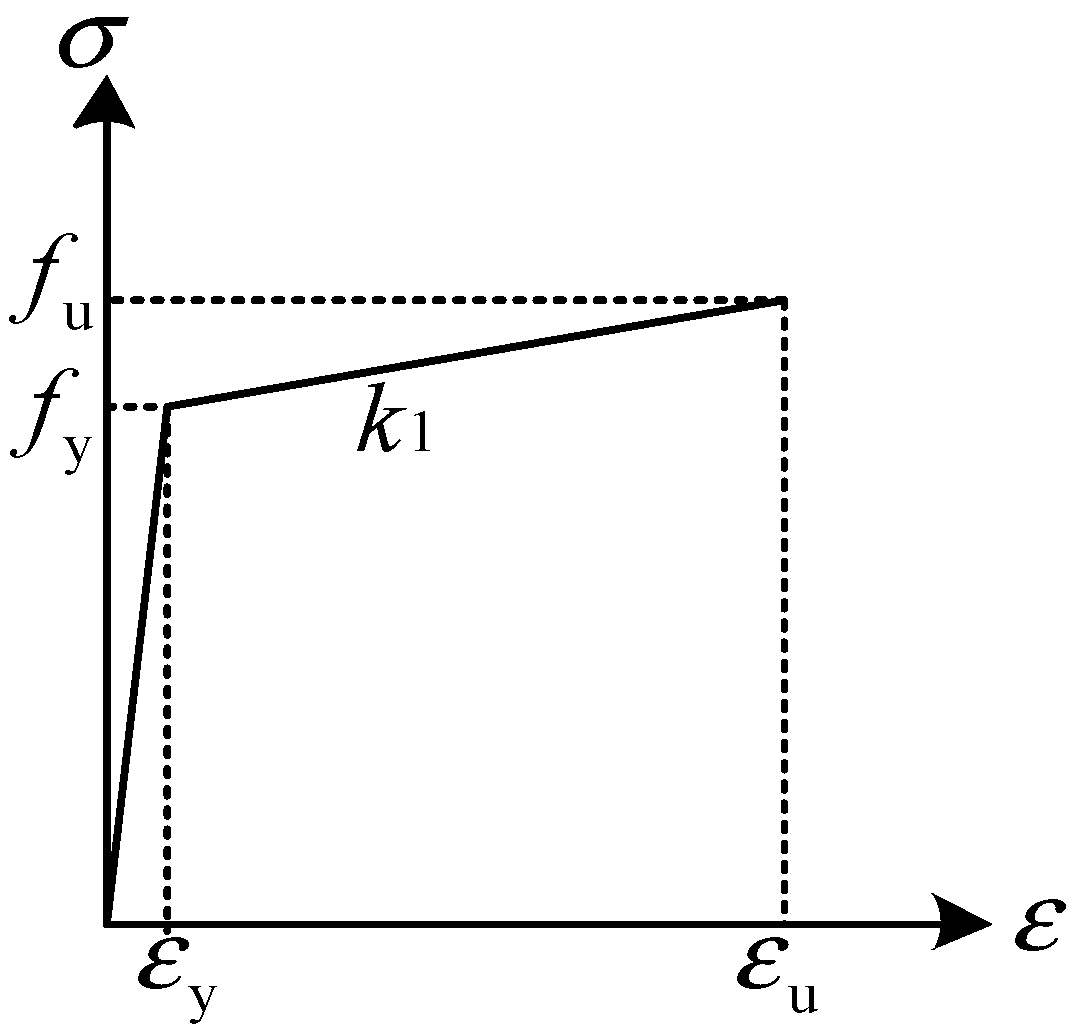
2.1.1. Constitutive Model of Steel
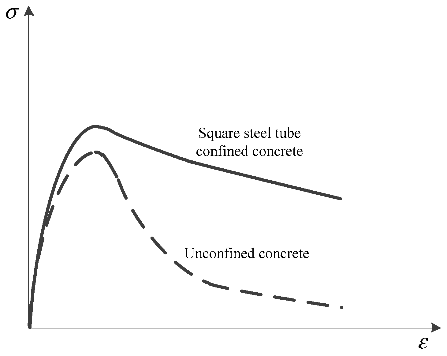
2.1.2. Confined Constitutive Model of Concrete with a Square Steel Tube
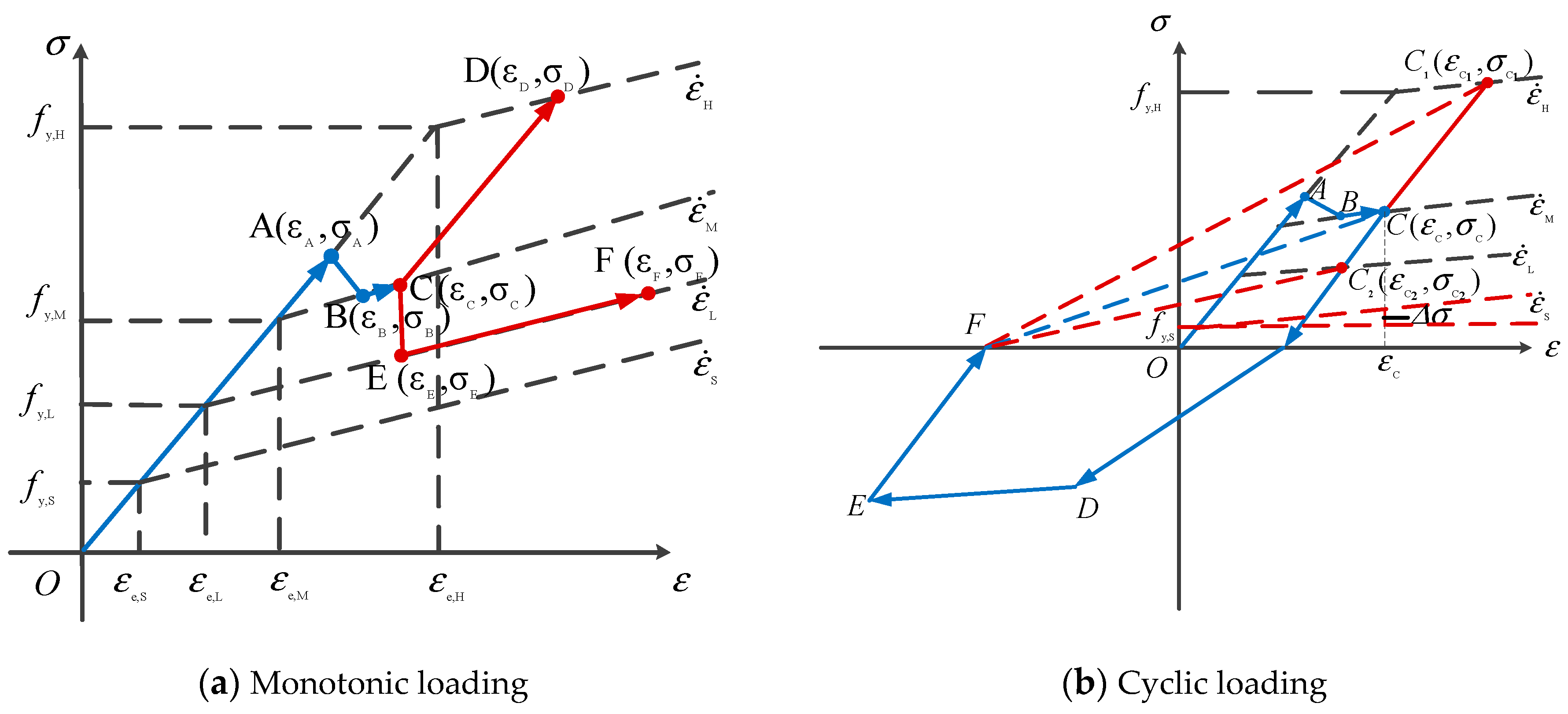
2.2. Strain Rate Effect
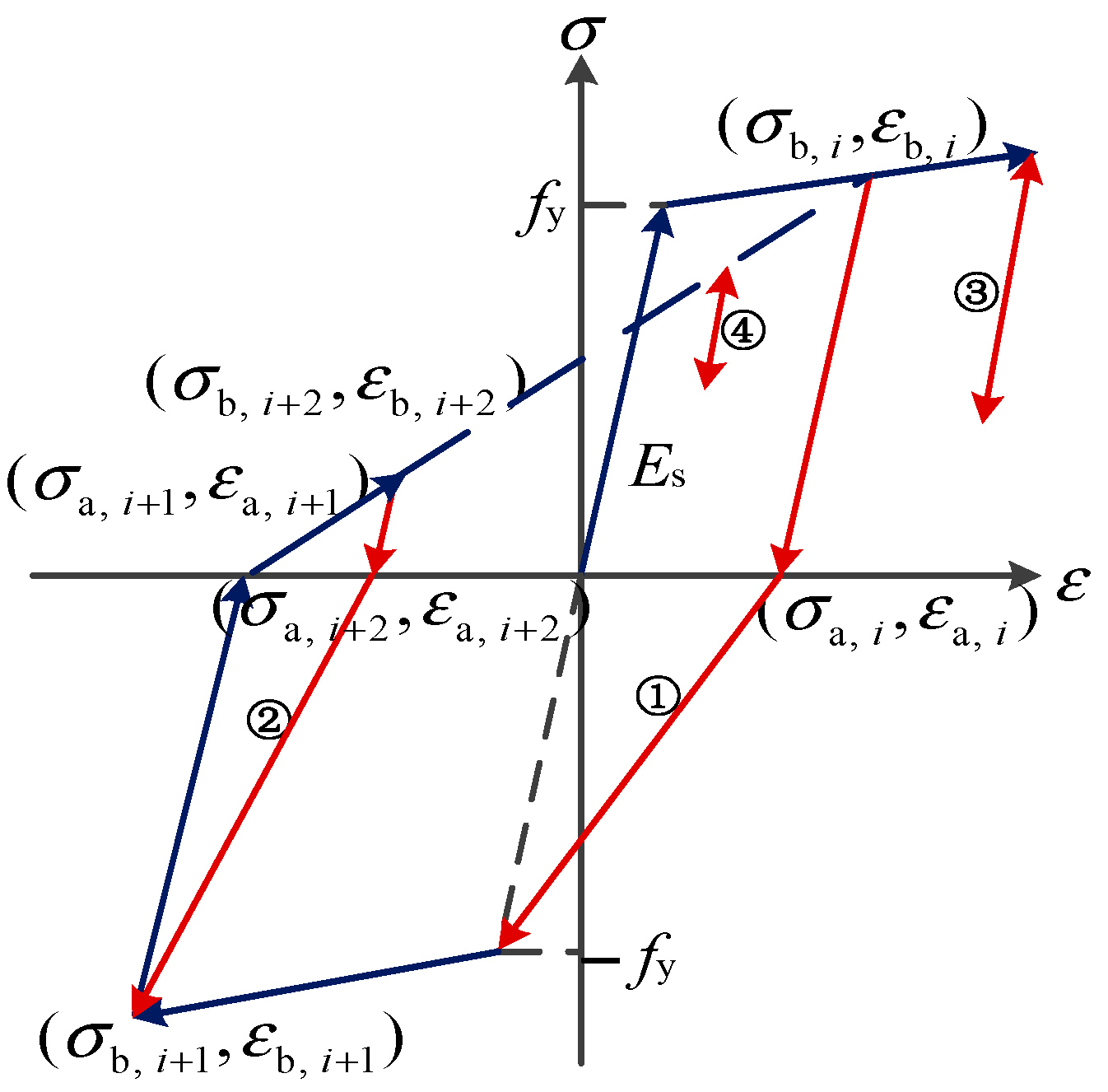
2.2.1. Strain Rate Effect of Steel
2.2.2. Strain Rate Effect of Concrete
3. Effect of Strain Rate and BRB on Seismic Response of a CFST Frame Structure
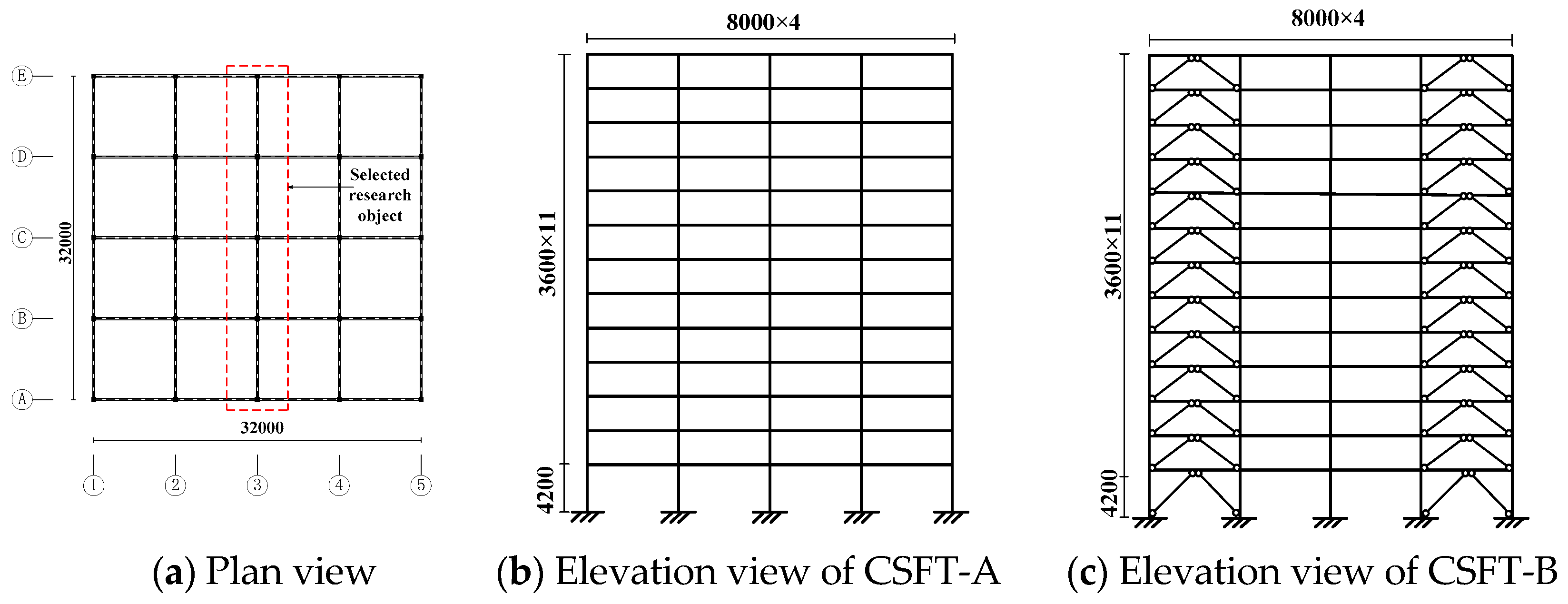
3.1. Description of the Finite Element Model
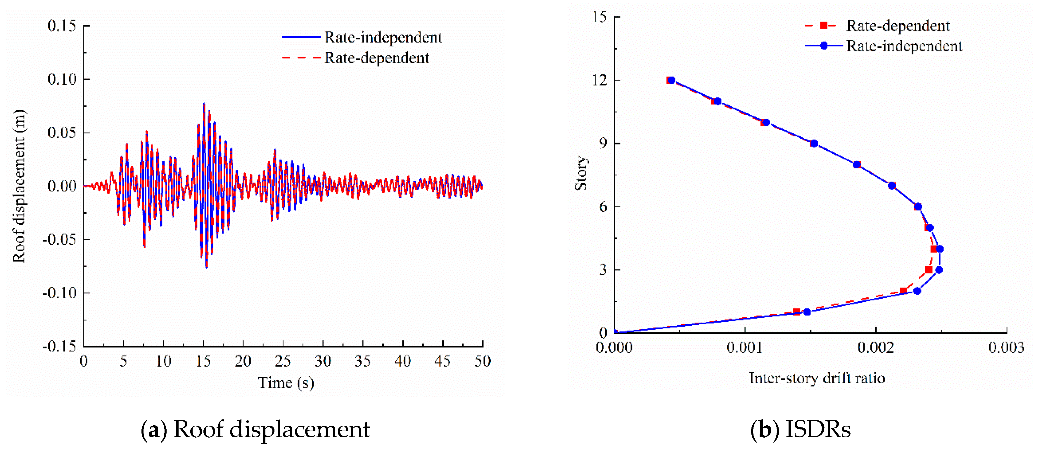
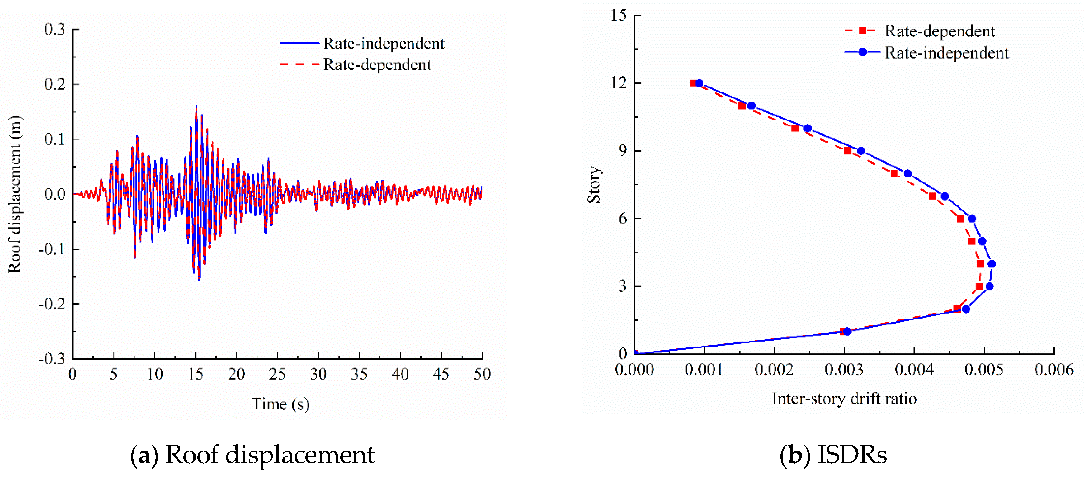
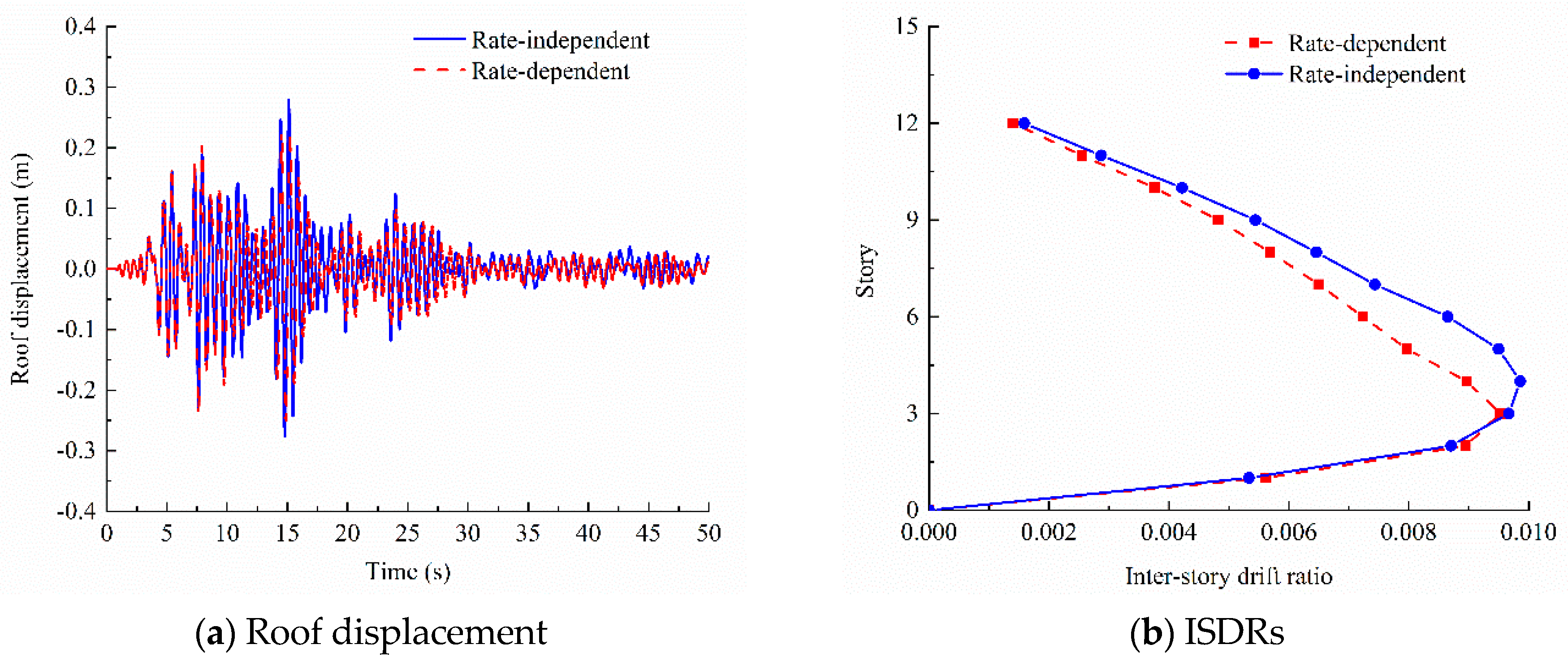
3.2. Analysis of the Influence of the Strain Rate on the Seismic Response of the CFST Structure
3.3. Influence of BRBs on the Seismic Response of the CFST Structure
4. Seismic Response CFST Structure with BRBs under Earthquake Sequences
4.1. Sequence-Type Ground Motion
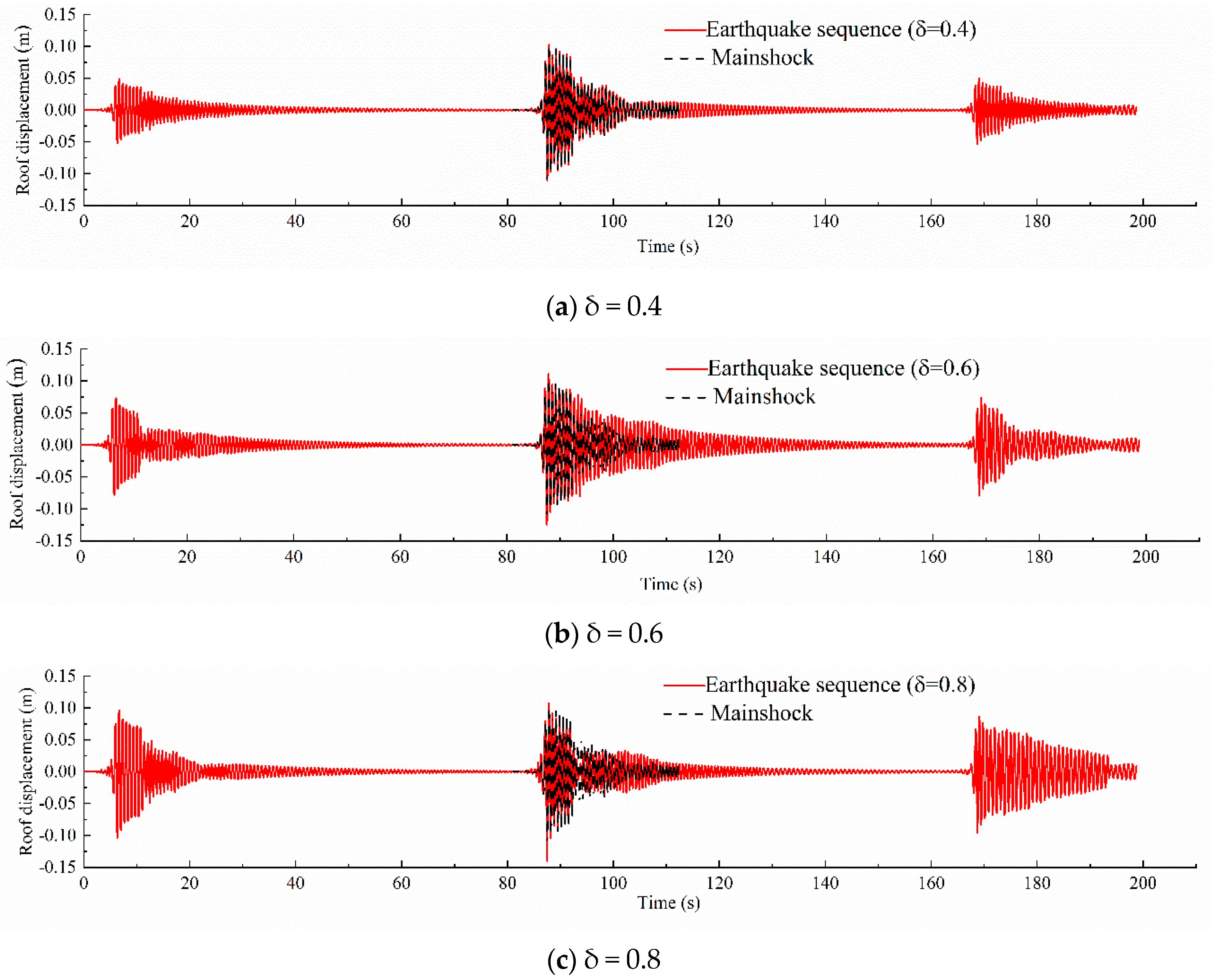
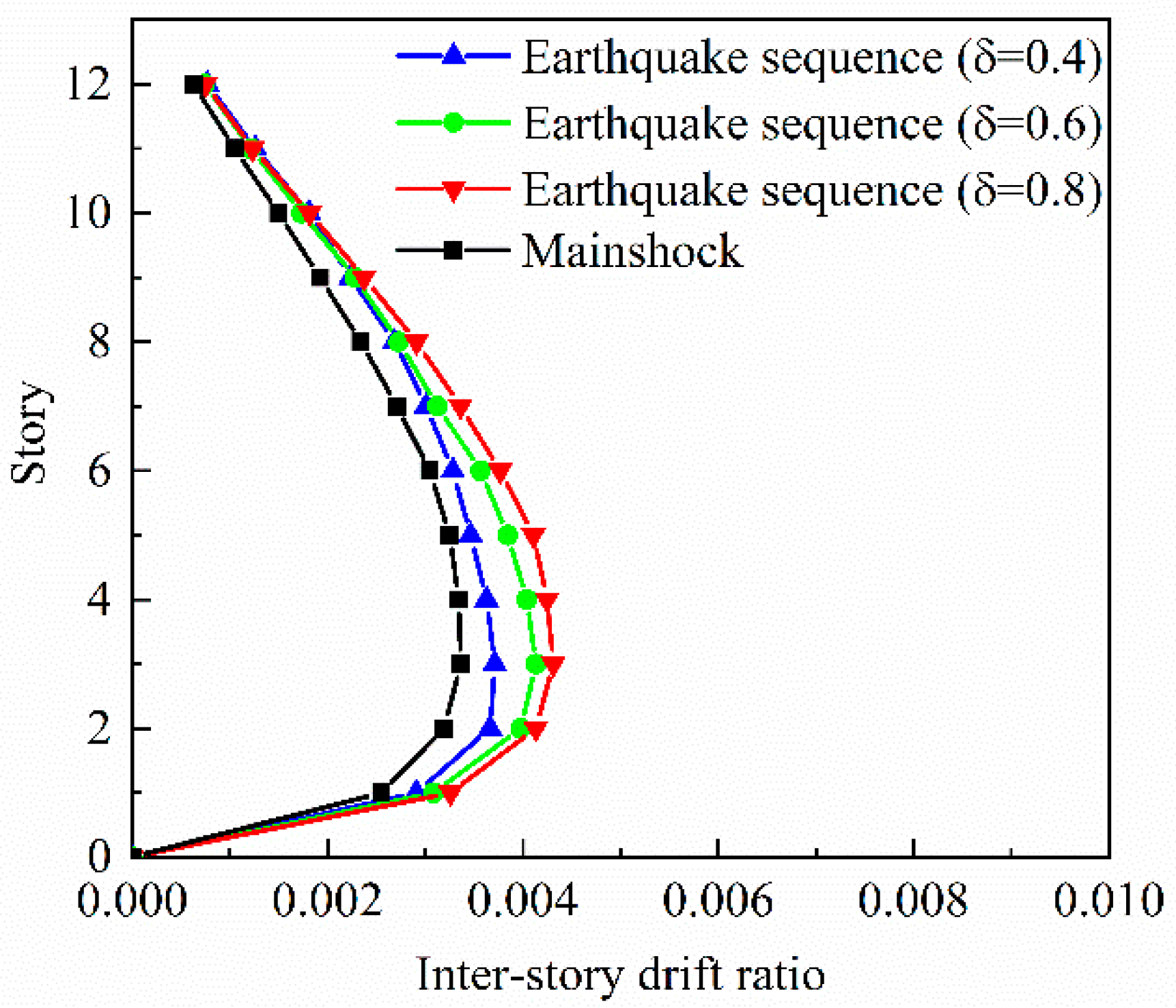
4.2. Nonlinear Response Analysis under Sequence-Type Ground Motion
5. Fragility Analysis of CFST with BRBs under Earthquake Sequences
5.1. Probabilistic Seismic Demand Model (PSDM)
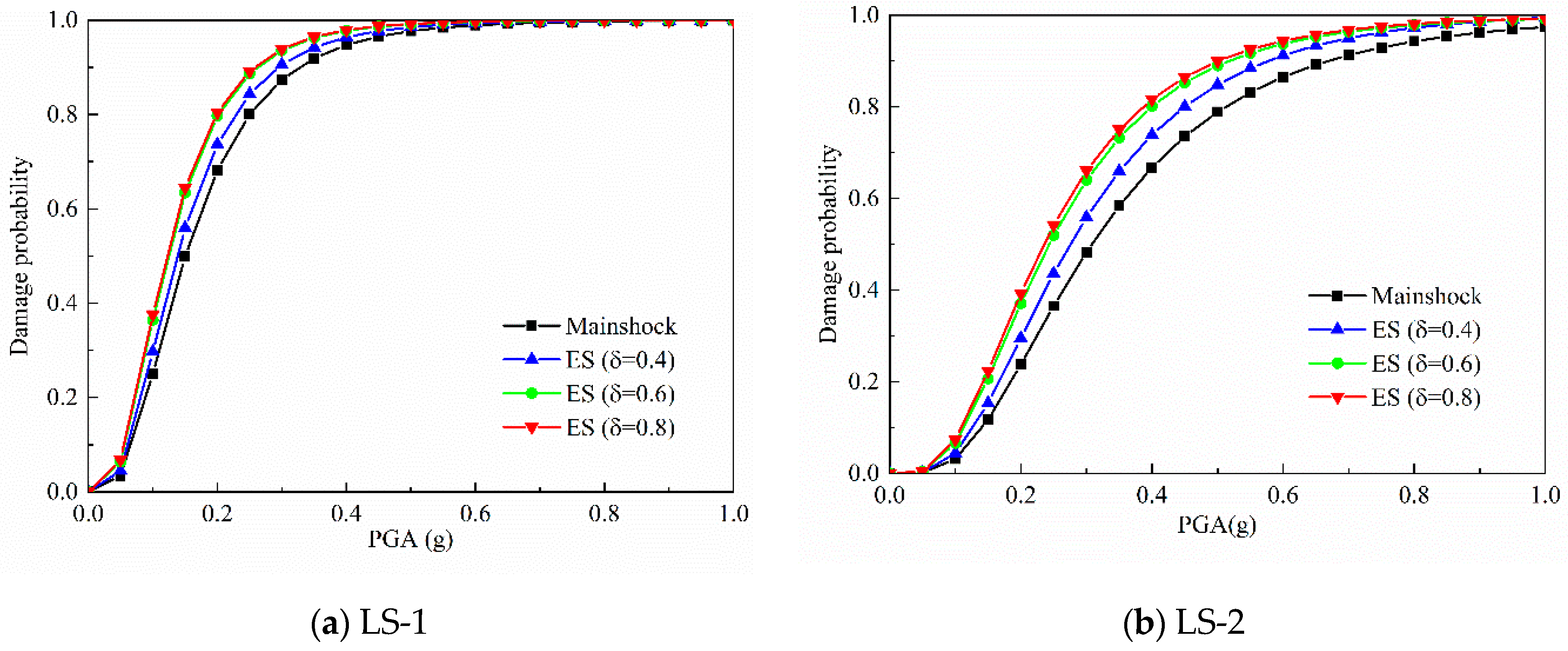
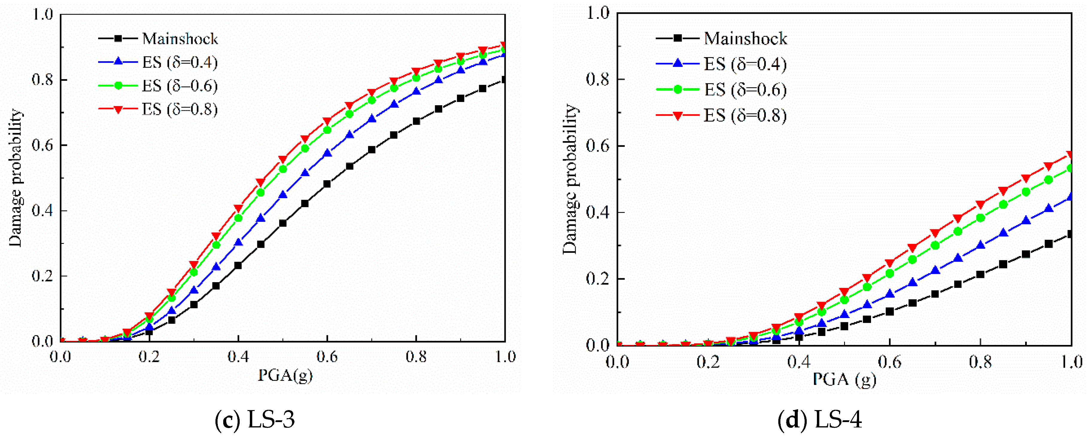
5.2. Results and Analysis
6. Conclusions
Author Contributions
Funding
Acknowledgments
Conflicts of Interest
References
- Bai, Y.; Wang, J.; Liu, Y. Thin-walled CFST columns for enhancing seismic collapse performance of high-rise steel frames. Appl. Sci. 2017, 7, 53. [Google Scholar] [CrossRef] [Green Version]
- Zhang, J.; Li, Y.; Zheng, Y. Seismic damage investigation of spatial frames with steel beams connected to L-shaped concrete-filled steel tubular (CFST) columns. Appl. Sci. 2018, 8, 1713. [Google Scholar] [CrossRef] [Green Version]
- Jia, S.Z.; Cao, W.L.; Liu, Z.B. Experimental study on a prefabricated lightweight concrete-filled steel tubular framework composite slab structure subjected to reversed cyclic loading. Appl. Sci. 2019, 9, 1264. [Google Scholar]
- Sabelli, R.; Mahin, S.; Chang, C. Seismic demands on steel braced frame buildings with buckling-restrained braces. Eng. Struct. 2003, 25, 655–666. [Google Scholar] [CrossRef]
- Fahnestock, L.A.; Sause, R.; Ricles, J.M. Seismic response and performance of buckling-restrained braced frames. J. Struct. Eng. 2007, 133, 1195–1204. [Google Scholar] [CrossRef]
- Ren, F.; Zhou, Y.; Chen, G. Experimental study on seismic performance of concrete-filled steel tabular frame-shear wall structure with buckling-resistant braces. Struct. Des. Tall Spec. 2015, 24, 73–95. [Google Scholar] [CrossRef]
- Wu, Y.; Song, W.; Zhao, W. An experimental study on dynamic mechanical properties of fiber-reinforced concrete under different strain rates. Appl. Sci. 2018, 8, 1904. [Google Scholar] [CrossRef] [Green Version]
- Atchley, B.L.; Furr, H.L. Strength and energy absorption capabilities of plain concrete under dynamic and static loadings. Am. Inst. Phys. Conf. Ser. 1967, 378, 268–274. [Google Scholar]
- Chang, K.C.; Lee, G.C. Strain rate effect on structural steel under cyclic loading. J. Eng. Mech. 1987, 113, 1292–1301. [Google Scholar] [CrossRef]
- Wakabayshi, M. Dynamic Loading Effects on the Structural Performance of Concrete and Steel Materials and Beams. In Proceedings of the Seventh World Conference on Earthquake Engineering, Istanbul, Turkey, 8–13 September 1980; Volume 6, pp. 271–278. [Google Scholar]
- Filiatrault, A.; Holleran, M. Stress-strain behavior of reinforcing steel and concrete under seismic strain rates and low temperatures. Mater. Struct. 2001, 34, 235–239. [Google Scholar] [CrossRef]
- Fu, H.C.; Erki, M.A.; Seckin, M. Review of effects of loading rate on reinforced concrete. J. Struct. Eng. 1991, 117, 3660–3679. [Google Scholar] [CrossRef]
- Malvar, L.J.; Ross, C.A. Review of strain rate effects for concrete in tension. ACI Mater. J. 1998, 95, 435–439. [Google Scholar]
- Bischoff, P.H.; Perry, S.H. Compressive behaviour of concrete at high strain rates. Mater. Struct. 1991, 24, 425–450. [Google Scholar] [CrossRef]
- Bertero, V.V.; Rea, D.; Mahin, S.A. Rate of Loading Effects on Uncracked and Repaired Reinforced Concrete Members. In Proceedings of the Fifth World Conference on Earthquake Engineering, Rome, Italy, 25–29 June 1973; Volume 1, pp. 1461–1470. [Google Scholar]
- Li, M.; Li, H. Effects of strain rate on reinforced concrete structure under seismic loading. Adv. Struct. Eng. 2012, 15, 461–475. [Google Scholar] [CrossRef]
- Li, H.N.; Li, M. Experimental and numerical study on dynamic properties of RC beam. Mag. Concr. Res. 2013, 65, 744–756. [Google Scholar] [CrossRef]
- Wang, D.; Li, H.N.; Li, G. Experimental tests on reinforced concrete columns under multi-dimensional dynamic loadings. Const. Build. Mater. 2013, 47, 1167–1181. [Google Scholar] [CrossRef]
- Carrillo, J.; Alcocer, S.M. Experimental investigation on dynamic and quas-static behavior of low-rise reinforced concrete walls. Earthq. Eng. Struct. Dyn. 2013, 42, 635–652. [Google Scholar] [CrossRef]
- Asprone, D.; Frascadore, R.; Ludovico, M.D. Influence of strain rate on the seismic response of RC structure. Eng. Struct. 2012, 35, 29–36. [Google Scholar] [CrossRef]
- Zhang, H.; Li, H.N.; Li, C.; Cao, G.W. Experimental and numerical investigations on seismic responses of reinforced concrete structures considering strain rate effect. Const. Build. Mater. 2018, 173, 672–686. [Google Scholar] [CrossRef]
- Luco, N.; Bazzurro, P.; Cornell, C.A. Dynamic Versus Static Computation of the Residual Capacity of a Mainshock-Damaged Building to Withstand an Aftershock. In Proceedings of the 13th World Conference on Earthquake Engineering, Auckland, New Zealand, 1–6 August 2004. [Google Scholar]
- Sarno, L.D. Effects of multiple earthquakes on inelastic structural response. Eng. Struct. 2013, 56, 673–681. [Google Scholar] [CrossRef]
- Ruiz-García, J.; Aguilar, J.D. Influence of modeling assumptions and aftershock hazard level in the seismic response of post-mainshock steel framed buildings. Eng. Struct. 2017, 140, 437–446. [Google Scholar] [CrossRef]
- Fragiacomo, M.; Amadio, C.; Macorini, L. Seismic response of steel frames under repeated earthquake ground motions. Eng. Struct. 2004, 26, 2021–2035. [Google Scholar] [CrossRef]
- Duerr, K. Seismic Vulnerability Assessment and Retrofit Optimization of Non-Code Conforming Buildings with Consideration of Mainshock-Aftershock Earthquake. Master’s Thesis, The University of British Columbia, Vancouver, BC, Canada, 2014. [Google Scholar]
- Goda, K.; Salami, M.R. Inelastic seismic demand estimation of wood-frame houses subjected to mainshock-aftershock sequences. Bull. Earthq. Eng. 2014, 12, 855–874. [Google Scholar] [CrossRef]
- Han, R.; Li, Y.; Lindt, J.V.D. Impact of aftershocks and uncertainties on the seismic evaluation of non-ductile reinforced concrete frame buildings. Eng. Struct. 2015, 100, 149–163. [Google Scholar] [CrossRef]
- Song, R.; Li, Y.; Van, D.L.J.W. Loss estimation of steel buildings to earthquake mainshock–aftershock sequences. Struct. Saf. 2016, 61, 1–11. [Google Scholar] [CrossRef] [Green Version]
- Ellingwood, B.R. Earthquake risk assessment of building structures. Reliab. Eng. Syst. Saf. 2001, 74, 251–262. [Google Scholar] [CrossRef]
- Sasani, M.; Kiureghian, A.D. Seismic fragility of RC structural walls: Displacement approach. J. Struct. Eng. 2001, 127, 219–228. [Google Scholar] [CrossRef]
- Ryu, H.; Luco, N.; Uma, S.; Liel, A. Developing Fragilities for Mainshock-Damaged Structures through Incremental Dynamic Analysis. In Proceedings of the 9th Pacific Conference on Earthquake Engineering, Auckland, New Zealand, 14–16 April 2011. [Google Scholar]
- Gardoni, P.; Kiureghian, A.; Mosalam, K.M. Probabilistic capacity models and fragility estimates for reinforced concrete columns based on experimental observations. J. Eng. Mech. 2002, 128, 1024–1038. [Google Scholar] [CrossRef]
- Li, C.; Hao, H.; Li, H. Seismic fragility analysis of reinforced concrete bridges with chloride induced corrosion subjected to spatially varying ground motions. Int. J. Struct. Stab. Dyn. 2016, 16, 1550010. [Google Scholar] [CrossRef]
- Li, C.; Li, H.N.; Hao, H. Seismic fragility analyses of sea-crossing cable-stayed bridges subjected to multi-support ground motions on offshore sites. Eng. Struct. 2018, 165, 441–456. [Google Scholar] [CrossRef]
- Li, Q.; Ellingwood, B.R. Performance evaluation and damage assessment of steel frame buildings under main shock-aftershock earthquake sequences. Earthq. Eng. Struct. Dyn. 2010, 36, 405–427. [Google Scholar] [CrossRef]
- Abdelnaby, A.E.; Elnashai, A.S. Performance of degrading reinforced concrete frame systems under the Tohoku and Christchurch earthquake sequences. J. Earthq. Eng. 2014, 18, 1009–1036. [Google Scholar] [CrossRef]
- Jeon, J.S.; DesRoches, R.; Lowes, L.N. Framework of aftershock fragility assessment–case studies: Older California reinforced concrete building frames. Earthq. Eng. Struct. Dyn. 2015, 44, 2617–2636. [Google Scholar] [CrossRef]
- Li, Y.; Song, R.; Van De, L.J.W. Collapse fragility of steel structures subjected to earthquake mainshock-aftershock sequences. J. Struct. Eng. 2014, 140, 04014095. [Google Scholar] [CrossRef]
- National Standards of the People’s Republic of China. Code for Design of Concrete Structures; GB 50010-2010; Standards Press of China: Beijing, China, 2010.
- Clough, R.W.; Johnson, S.B. Effect of stiffness degradation on earthquake ductility requirements. In Proceedings of the Japan Earthquake Engineering Symposium, Tokyo, Japan, October 1966; pp. 195–198. Available online: https://link.springer.com/article/10.1007/s11803-006-0631-0 (accessed on 24 November 2019).
- Han, L.H. Theory and Practice of Concrete Filled Steel Tubular Structure, 3rd ed.; Science Press: Beijing, China, 2007; pp. 170–186. [Google Scholar]
- Zhang, X.H.; Duan, Z.D.; Zhang, C.W. Numerical simulation of dynamic response for steel frame structures subjected to blast load. Trans. Tianjin Univ. 2008, 14, 523–529. [Google Scholar] [CrossRef]
- Gholipour, G.; Zhang, C.W.; Mousavi, A. Effects of axial load on nonlinear response of RC columns subjected to lateral impact load: Ship-pier collision. Eng. Fail. Anal. 2018, 91, 397–418. [Google Scholar] [CrossRef]
- Zhang, C.W.; Gholipour, G.; Mousavi, A.A. Nonlinear dynamic behavior of simply-supported RC beams subjected to combined impact-blast loading. Eng. Struct. 2019, 181, 124–142. [Google Scholar] [CrossRef]
- Xiao, S.; Li, H.; Monteiro, P.J.M. Influence of strain rates and loading histories on the compressive damage behaviour of concrete. Mag. Concr. Res. 2011, 63, 915–926. [Google Scholar] [CrossRef]
- Zhang, H.; Li, H.N.; Cao, G.W. Fiber beam element model for reinforced concrete structures considering strain rate effects. J. Build. Struct. 2019, 40, 103–112. [Google Scholar]
- Yan, D.M.; Lin, G. Dynamic properties of concrete in direct tension. Cem. Concr. Res. 2006, 36, 1371–1378. [Google Scholar] [CrossRef]
- Hao, X.Y.; Li, H.N.; Li, G. Experimental investigation of steel structure with innovative H-type steel unbuckling braces. Struct. Des. Tall Spec. 2014, 23, 1064–1082. [Google Scholar] [CrossRef]
- Charney, F.A.; Marshall, J. A Comparison of the Krawinkler and scissors models for including beam-column joint deformations in the analysis of moment-resisting steel frames. Eng. J. AISC 2006, 43, 31–48. [Google Scholar]
- Gutenberg, B.; Richter, C.F. Seismicity of the Earth and Associated Phenomena, 2nd ed.; Princeton University Press: Princeton, NJ, USA, 2013; pp. 236–244. [Google Scholar]
- Hatzigeorgiou, G.D.; Beskos, D.E. Inelastic displacement ratios for SDOF structures subjected to repeated earthquakes. Eng. Struct. 2009, 31, 2744–2755. [Google Scholar] [CrossRef]
- Mackie, K.; Stojadinović, B. Fragility Basis for California Highway Overpass Bridge Seismic Decision Making; PEER Report No. 2005/02; Pacific Earthquake Engineering Research Center, University of California: Berkeley, CA, USA, 2005. [Google Scholar]
- Cornell, C.A. The probabilistic basis for the 2000SAC/FEMA steel moment frame guidelines. J. Struct. Eng. 2002, 128, 526–533. [Google Scholar] [CrossRef] [Green Version]
- National Standards of the People’s Republic of China. Code for Seismic Design of Buildings; GB 50011-2010; Standards Press of China: Beijing, China, 2010.
- China Association for Engineering Construction Standardization. Code for Design of Steel-Concrete Hybrid Structures for High-Rise Building; CECS 230:2008; China Association for Engineering Construction Standardization: Beijing, China, 2008.


| Input Motions | PGA (g) | Roof Displacement | ISDR (10−3) | ||||
|---|---|---|---|---|---|---|---|
| Rate- Independent (mm) | Rate- Dependent (mm) | Difference (%) | Rate- Independent (10−3) | Rate- Dependent (10−3) | Difference (%) | ||
| San Fernando | 0.1 | 25.68 | 25.46 | −0.9 | 0.85 | 0.85 | - |
| 0.2 | 51.36 | 50.39 | −1.9 | 1.70 | 1.66 | −2.4 | |
| 0.3 | 77.10 | 75.42 | −2.2 | 2.53 | 2.48 | −2.0 | |
| 0.4 | 102.80 | 98.96 | −3.7 | 3.39 | 3.25 | −4.1 | |
| 0.5 | 128.59 | 122.68 | −4.6 | 4.24 | 4.04 | −4.7 | |
| 0.6 | 154.46 | 147.67 | −4.4 | 5.09 | 4.86 | −4.5 | |
| 0.7 | 180.49 | 172.38 | −4.5 | 5.94 | 5.69 | −4.2 | |
| 0.8 | 206.54 | 196.52 | −4.9 | 6.81 | 6.51 | −4.4 | |
| 0.9 | 233.30 | 220.98 | −5.3 | 7.87 | 7.44 | −5.5 | |
| 1.0 | 259.10 | 236.14 | −8.9 | 8.92 | 8.45 | −5.3 | |
| Taft | 0.1 | 38.75 | 38.56 | −0.5 | 1.24 | 1.24 | - |
| 0.2 | 77.47 | 76.32 | −1.5 | 2.49 | 2.44 | −2.0 | |
| 0.3 | 118.76 | 115.04 | −3.1 | 3.73 | 3.64 | −2.4 | |
| 0.4 | 161.38 | 154.76 | −4.1 | 5.11 | 4.95 | −3.1 | |
| 0.5 | 204.14 | 196.36 | −3.8 | 6.56 | 6.17 | −5.9 | |
| 0.6 | 247.27 | 236.75 | −4.3 | 7.83 | 7.45 | −4.9 | |
| 0.7 | 272.47 | 244.68 | −10.2 | 9.29 | 8.65 | −6.9 | |
| 0.8 | 279.05 | 250.99 | −10.1 | 9.86 | 9.53 | −3.3 | |
| 0.9 | 287.44 | 269.36 | −6.3 | 10.67 | 10.11 | −5.2 | |
| 1.0 | 308.01 | 285.21 | −7.4 | 12.19 | 11.69 | −4.1 | |
| Gengmaa | 0.1 | 8.09 | 8.09 | - | 0.27 | 0.27 | - |
| 0.2 | 16.24 | 16.02 | −1.4 | 0.56 | 0.55 | −1.8 | |
| 0.3 | 24.31 | 23.54 | −3.2 | 0.83 | 0.81 | −2.4 | |
| 0.4 | 32.40 | 31.24 | −3.6 | 1.11 | 1.06 | −4.5 | |
| 0.5 | 40.55 | 39.11 | −3.6 | 1.39 | 1.34 | −3.6 | |
| 0.6 | 48.71 | 46.73 | −4.1 | 1.67 | 1.59 | −4.8 | |
| 0.7 | 56.79 | 54.45 | −4.1 | 1.95 | 1.85 | −5.1 | |
| 0.8 | 64.96 | 61.84 | −4.8 | 2.23 | 2.11 | −5.4 | |
| 0.9 | 73.07 | 67.94 | −7.0 | 2.50 | 2.39 | −4.4 | |
| 1.0 | 81.22 | 76.14 | −6.3 | 2.79 | 2.67 | −4.3 | |
| Input Motions | PGA (g) | Roof Displacement (mm) | ISDR (10−3) | ||||
|---|---|---|---|---|---|---|---|
| CFST-A | CFST-B | Difference (%) | CFST-A | CFST-B | Difference (%) | ||
| San Fernando | 0.1 | 25.46 | 19.34 | −24.0 | 0.85 | 0.64 | −24.7 |
| 0.2 | 50.39 | 38.65 | −23.3 | 1.66 | 1.27 | −23.5 | |
| 0.3 | 75.42 | 57.77 | −23.4 | 2.48 | 1.91 | −23.0 | |
| 0.4 | 98.96 | 76.94 | −22.3 | 3.25 | 2.53 | −22.2 | |
| 0.5 | 122.68 | 95.91 | −21.8 | 4.04 | 3.17 | −21.5 | |
| 0.6 | 147.67 | 114.78 | −22.3 | 4.86 | 3.80 | −21.8 | |
| 0.7 | 172.38 | 133.86 | −22.3 | 5.69 | 4.45 | −21.8 | |
| 0.8 | 196.52 | 152.72 | −22.3 | 6.51 | 5.09 | −21.8 | |
| 0.9 | 220.98 | 171.80 | −22.3 | 7.44 | 5.71 | −23.3 | |
| 1.0 | 236.14 | 190.80 | −19.2 | 8.45 | 6.32 | −25.2 | |
| Taft | 0.1 | 38.56 | 22.95 | −40.5 | 1.24 | 0.76 | −38.7 |
| 0.2 | 76.32 | 45.75 | −40.1 | 2.44 | 1.49 | −38.9 | |
| 0.3 | 115.04 | 67.85 | −41.0 | 3.64 | 2.18 | −40.1 | |
| 0.4 | 154.76 | 90.69 | −41.4 | 4.95 | 2.96 | −40.2 | |
| 0.5 | 196.36 | 113.21 | −42.3 | 6.17 | 3.71 | −39.9 | |
| 0.6 | 236.75 | 135.69 | −42.7 | 7.45 | 4.48 | −39.9 | |
| 0.7 | 244.68 | 158.59 | −35.2 | 8.65 | 5.21 | −39.8 | |
| 0.8 | 250.99 | 182.60 | −27.2 | 9.53 | 6.03 | −36.7 | |
| 0.9 | 269.36 | 202.90 | −24.7 | 10.11 | 6.68 | −33.9 | |
| 1.0 | 285.21 | 226.60 | −20.5 | 11.69 | 7.62 | −34.8 | |
| Gengmaa | 0.1 | 8.09 | 6.48 | −19.9 | 0.27 | 0.20 | −25.9 |
| 0.2 | 16.02 | 12.96 | −19.1 | 0.55 | 0.40 | −27.3 | |
| 0.3 | 23.54 | 19.30 | −18.0 | 0.81 | 0.61 | −24.7 | |
| 0.4 | 31.24 | 25.77 | −17.5 | 1.06 | 0.79 | −25.5 | |
| 0.5 | 39.11 | 32.28 | −17.5 | 1.34 | 0.98 | −26.9 | |
| 0.6 | 46.73 | 38.75 | −17.1 | 1.59 | 1.21 | −23.9 | |
| 0.7 | 54.45 | 45.14 | −17.1 | 1.85 | 1.38 | −25.4 | |
| 0.8 | 61.84 | 51.67 | −16.4 | 2.11 | 1.55 | −26.5 | |
| 0.9 | 67.94 | 58.35 | −14.1 | 2.39 | 1.75 | −26.8 | |
| 1.0 | 76.14 | 64.73 | −15.0 | 2.67 | 1.98 | −25.8 | |
| Input Motions | PGA (g) | Roof Displacement (mm) | ||||||
|---|---|---|---|---|---|---|---|---|
| Mainshock Only | Earthquake Sequence (δ = 0.4) | Difference (%) | Earthquake Sequence (δ = 0.6) | Difference (%) | Earthquake Sequence (δ = 0.8) | Difference (%) | ||
| M-AGW | 0.032 | 10.12 | 11.93 | 17.82 | 12.94 | 27.84 | 14.11 | 39.41 |
| A-CAT | 0.042 | 21.14 | 22.54 | 6.62 | 23.61 | 11.68 | 24.82 | 17.41 |
| A-STP | 0.049 | 23.18 | 26.65 | 14.95 | 26.66 | 15.00 | 31.47 | 35.75 |
| HO6 | 0.060 | 13.42 | 14.61 | 8.88 | 15.75 | 17.42 | 18.79 | 40.08 |
| A-CTS | 0.062 | 19.74 | 20.84 | 5.55 | 22.82 | 15.60 | 26.22 | 32.80 |
| A-HAR | 0.070 | 47.32 | 48.08 | 1.62 | 51.35 | 8.53 | 57.41 | 21.35 |
| H-CO8 | 0.100 | 70.99 | 74.70 | 5.24 | 90.07 | 26.88 | 94.47 | 33.07 |
| H-CC4 | 0.115 | 36.09 | 43.62 | 20.88 | 52.29 | 44.88 | 53.64 | 48.62 |
| H-CAL | 0.128 | 19.19 | 24.74 | 28.93 | 28.43 | 48.13 | 31.99 | 66.70 |
| H-CMP | 0.144 | 69.19 | 73.94 | 6.87 | 86.52 | 25.04 | 92.26 | 33.34 |
| BRA | 0.160 | 28.61 | 30.70 | 7.31 | 33.11 | 15.73 | 36.55 | 27.75 |
| M-GMR | 0.184 | 12.15 | 15.98 | 31.56 | 20.19 | 66.18 | 20.40 | 67.90 |
| M-G03 | 0.194 | 24.76 | 27.44 | 10.81 | 27.34 | 10.41 | 27.47 | 10.93 |
| M-G02 | 0.200 | 42.15 | 53.57 | 27.09 | 49.71 | 17.94 | 56.94 | 35.09 |
| A-DWN | 0.215 | 98.21 | 107.62 | 9.58 | 124.44 | 26.71 | 124.92 | 27.20 |
| FLE | 0.237 | 56.93 | 68.62 | 20.54 | 79.27 | 39.24 | 89.22 | 56.71 |
| C08 | 0.259 | 88.21 | 90.75 | 2.87 | 95.97 | 8.80 | 106.57 | 20.82 |
| H-CHI | 0.269 | 153.27 | 180.49 | 17.76 | 194.00 | 26.58 | 235.07 | 53.37 |
| A-BIR | 0.299 | 85.14 | 106.52 | 25.11 | 123.55 | 45.11 | 134.30 | 57.73 |
| I-ELC | 0.309 | 205.51 | 208.51 | 1.46 | 229.05 | 11.45 | 255.67 | 24.41 |
| A-CAS | 0.322 | 103.16 | 110.72 | 7.33 | 124.45 | 20.64 | 140.07 | 35.78 |
| H-DLT | 0.349 | 108.68 | 123.62 | 13.75 | 134.69 | 23.93 | 159.73 | 46.97 |
| HOL | 0.358 | 189.52 | 194.36 | 2.55 | 207.12 | 9.29 | 218.26 | 15.17 |
| CAP | 0.395 | 120.07 | 122.69 | 2.18 | 126.24 | 5.14 | 143.24 | 19.30 |
| G04 | 0.413 | 108.79 | 132.15 | 21.47 | 169.48 | 55.79 | 187.37 | 72.23 |
| G03 | 0.547 | 169.79 | 174.69 | 2.89 | 180.37 | 6.23 | 259.14 | 52.62 |
| SCS | 0.612 | 430.69 | 504.98 | 17.25 | 598.28 | 38.91 | 697.79 | 62.02 |
| H-BCR | 0.780 | 197.14 | 214.99 | 9.05 | 243.75 | 23.64 | 259.11 | 31.44 |
| RRS | 0.834 | 659.33 | 717.68 | 8.85 | 794.27 | 20.47 | 837.11 | 26.96 |
| SPV | 0.939 | 272.37 | 286.98 | 5.36 | 292.49 | 7.39 | 356.46 | 30.87 |
| Input Motions | PGA (g) | ISDR (10−3) | ||||||
|---|---|---|---|---|---|---|---|---|
| Mainshock Only | Earthquake Sequence (δ = 0.4) | Difference (%) | Earthquake Sequence (δ = 0.6) | Difference (%) | Earthquake Sequence (δ = 0.8) | Difference (%) | ||
| M-AGW | 0.032 | 0.42 | 0.52 | 21.92 | 0.58 | 36.44 | 0.62 | 45.62 |
| A-CAT | 0.042 | 0.60 | 0.72 | 20.02 | 0.77 | 27.58 | 0.79 | 31.60 |
| A-STP | 0.049 | 0.79 | 0.86 | 9.01 | 0.87 | 10.41 | 1.04 | 31.30 |
| HO6 | 0.060 | 0.37 | 0.40 | 7.62 | 0.44 | 18.10 | 0.47 | 24.97 |
| A-CTS | 0.062 | 0.60 | 0.69 | 15.78 | 0.70 | 17.71 | 0.85 | 41.82 |
| A-HAR | 0.070 | 1.54 | 1.60 | 3.81 | 1.70 | 10.03 | 1.88 | 22.07 |
| H-CO8 | 0.100 | 2.30 | 2.46 | 6.89 | 2.95 | 28.33 | 3.24 | 41.06 |
| H-CC4 | 0.115 | 1.23 | 1.40 | 13.55 | 1.66 | 34.46 | 1.76 | 42.45 |
| H-CAL | 0.128 | 0.71 | 0.84 | 17.48 | 0.90 | 25.50 | 0.99 | 38.24 |
| H-CMP | 0.144 | 2.51 | 2.62 | 4.29 | 3.02 | 20.36 | 3.55 | 41.12 |
| BRA | 0.160 | 0.95 | 0.98 | 3.82 | 1.12 | 18.38 | 1.23 | 30.01 |
| M-GMR | 0.184 | 0.68 | 0.73 | 6.23 | 0.78 | 13.84 | 0.80 | 17.08 |
| M-G03 | 0.194 | 0.85 | 0.92 | 7.33 | 0.94 | 9.45 | 0.99 | 15.58 |
| M-G02 | 0.200 | 1.20 | 1.48 | 23.13 | 1.59 | 32.30 | 1.68 | 39.64 |
| A-DWN | 0.215 | 3.24 | 3.62 | 11.76 | 4.23 | 30.42 | 4.27 | 31.65 |
| FLE | 0.237 | 2.20 | 3.11 | 41.26 | 3.20 | 45.45 | 3.48 | 58.03 |
| C08 | 0.259 | 3.02 | 3.11 | 3.05 | 3.40 | 12.58 | 3.66 | 21.07 |
| H-CHI | 0.269 | 4.01 | 5.19 | 29.29 | 5.99 | 49.31 | 6.06 | 50.94 |
| A-BIR | 0.299 | 1.92 | 2.26 | 17.44 | 2.34 | 21.67 | 2.79 | 45.22 |
| I-ELC | 0.309 | 6.90 | 8.70 | 26.09 | 9.50 | 37.69 | 10.11 | 46.55 |
| A-CAS | 0.322 | 3.36 | 3.71 | 10.42 | 4.13 | 22.92 | 4.31 | 28.27 |
| H-DLT | 0.349 | 0.93 | 1.40 | 51.47 | 1.55 | 67.01 | 1.63 | 76.23 |
| HOL | 0.358 | 6.74 | 6.97 | 3.41 | 7.38 | 9.50 | 8.18 | 21.31 |
| CAP | 0.395 | 3.87 | 4.10 | 5.94 | 4.27 | 10.34 | 4.59 | 18.64 |
| G04 | 0.413 | 3.99 | 4.75 | 18.95 | 5.64 | 41.35 | 6.55 | 64.16 |
| G03 | 0.547 | 21.23 | 22.83 | 7.54 | 26.75 | 25.98 | 30.88 | 45.46 |
| SCS | 0.612 | 74.95 | 84.61 | 12.89 | 106.15 | 41.63 | 109.75 | 46.43 |
| H-BCR | 0.780 | 27.60 | 29.02 | 5.14 | 30.24 | 9.57 | 34.99 | 26.79 |
| RRS | 0.834 | 111.24 | 121.52 | 9.24 | 134.90 | 21.27 | 144.43 | 29.84 |
| SPV | 0.939 | 34.97 | 36.02 | 2.99 | 37.53 | 7.32 | 41.76 | 19.43 |
| Cases | Linear Regression Model | R2 | |
|---|---|---|---|
| Mainshock | ln(ISDRx) = −4.1604 + 0.96596 ln(PGA) | 0.76618 | 0.27845 |
| ES(δ = 0.4) | ln(ISDRax) = −4.03073 + 0.98723 ln(PGA) | 0.75449 | 0.28215 |
| ES(δ = 0.6) | ln(ISDRax) = −3.86207 + 1.01474 ln(PGA) | 0.77191 | 0.29486 |
| ES(δ = 0.8) | ln(ISDRax) = −3.79405 + 1.03846 ln(PGA) | 0.76804 | 0.31308 |
© 2019 by the authors. Licensee MDPI, Basel, Switzerland. This article is an open access article distributed under the terms and conditions of the Creative Commons Attribution (CC BY) license (http://creativecommons.org/licenses/by/4.0/).
Share and Cite
Zhang, H.; Li, C.; Jiang, S.-M.; Liu, P.-F.; Gao, Q.-M. Fragility Analysis of Concrete-Filled Steel Tubular Frame Structures with BRBs under Multiple Earthquakes Considering Strain Rate Effects. Appl. Sci. 2020, 10, 165. https://doi.org/10.3390/app10010165
Zhang H, Li C, Jiang S-M, Liu P-F, Gao Q-M. Fragility Analysis of Concrete-Filled Steel Tubular Frame Structures with BRBs under Multiple Earthquakes Considering Strain Rate Effects. Applied Sciences. 2020; 10(1):165. https://doi.org/10.3390/app10010165
Chicago/Turabian StyleZhang, Hao, Chao Li, Si-Meng Jiang, Peng-Fei Liu, and Qing-Meng Gao. 2020. "Fragility Analysis of Concrete-Filled Steel Tubular Frame Structures with BRBs under Multiple Earthquakes Considering Strain Rate Effects" Applied Sciences 10, no. 1: 165. https://doi.org/10.3390/app10010165