Two-Stage Stochastic Programming Scheduling Model for Hybrid AC/DC Distribution Network Considering Converters and Energy Storage System

Abstract

The development of DC distribution network technology has provided a more efficient way for renewable energy accommodation and flexible power supply. A two-stage stochastic scheduling model for the hybrid AC/DC distribution network is proposed to study the active-reactive power coordinated optimal dispatch. In this framework, the wind power scenario set is utilized to deal with its uncertainty in real time, which is integrated into the decision-making process at the first stage. The charging/discharging power of ESSs and the transferred active/reactive power by VSCs can be adjusted when wind power uncertainty is observed at the second stage. Moreover, the proposed model is transformed into a mixed integer second-order cone programming optimization problem by linearization and second-order cone relaxation techniques to solve. Finally, case studies are implemented on the modified IEEE 33-node AC/DC distribution system and the simulation results demonstrate the effectiveness of the proposed stochastic scheduling model and solving method.

1. Introduction

With the rapid growth of renewable energy and energy storage systems integrated in the distribution network, the development of a DC distribution network has drawn more and more attention [1]. Compared to the AC distribution network, the DC distribution network has the advantages of reducing active power losses, and improving the power quality and utilization rate of electric energy [2,3]. As a result, the hybrid AC/DC distribution network will become a new tendency of intelligent distribution network development in the future [4,5]. By combining the advantages of two kinds of distribution networks, the hybrid distribution network can achieve flexible power supply for different types of electric load and renewable energy accommodation [6,7].

To handle the variations of renewable energy and load demand, a multi-timescale coordinated stochastic voltage/var control approach was developed and a mixed-integer quadratic programming model was built for the IEEE 33-bus radial AC distribution [8]. The authors of [9] proposed a day-ahead reactive power dispatch method of AC distribution networks by considering power forecast errors of renewable energy, and a dynamic preliminary-coarse-fine adjustment strategy was designed to achieve the optimal scheduling of distributed generators (DGs) and capacitor banks (CBs).

At present, research of the hybrid AC/DC distribution network is in the elementary stage and needs to expand and deepen. Voltage source converters (VSCs) have been utilized to convert AC lines into DC lines to improve DG accommodations [10]. To realize the coordinated voltage regulation in a hybrid AC/DC distribution system, a priority-based real-time control strategy was proposed according to the voltage control effect of active-reactive power adjustment in [11]. Multiple battery energy storage systems (ESSs) have been considered in distribution networks for real-time voltage regulation in [12]. Furthermore, [13] proposed an optimal control management of ESSs to mitigate the fluctuation and intermittence of renewable energy. Taking into consideration prediction errors, the optimal operation of ESSs in a distribution system was developed and solved in a two-level framework to alleviate the net load uncertainties [14,15]. For the planning problems of ESSs, [16] introduced a new index to quantify wind power fluctuations, and the impact of different ESSs configurations on the solutions were analyzed. A scenario-based chance-constrained planning approach was developed to handle the joint planning of multiple technologies of ESSs, and an easy-to-implement variant of Benders decomposition algorithm was proposed to solve the chance-constrained optimization problem [17]. In order to improve the reliability of electricity supplies with wind power integration, a population meta-heuristics algorithm was adopted to determine the minimum capacity of kinetic energy storage in [18].

To consider the randomness and uncertainty of wind power output, this paper proposes a two-stage stochastic scheduling model to realize active-reactive power coordinated economic dispatch for the hybrid AC/DC distribution network with the integration of capacitor banks and an energy storage system. The first stage is to determine the power setpoints of generator units, switching number of CBs, and charging/discharging state of ESSs, and the second stage is to adjust the transferred active/reactive power of VSCs and charging/discharging power of ESSs based on the realized wind power scenarios. To sum up, the schematic framework of this study is shown in Figure 1, for which the corresponding research contents are described in the following sections.

The contributions of this paper can be summarized as follows:

(1) The capacitor bank, energy storage system, and voltage source converter are coordinated as the active adjustment measures simultaneously in the hybrid AC/DC distribution system. By this means, a comprehensive and practical framework considering active and reactive powers coordination dispatch is established.

(2) A two-stage stochastic programming model is established to achieve active-reactive power coordinated economic dispatch for the hybrid distribution system, in which wind power uncertainty is described as several wind power scenarios obtained by scenario generation and reduction techniques. As a result, the decision-making at the first stage not only depends on the day-ahead wind power predictions but is also affected by wind power uncertainty in the real-time scheduling stage. In other words, the realized wind power scenario set in real time is integrated into the decision process for the two-stage scheduling problem.

(3) The proposed stochastic programming model is a nonlinear optimization problem, which is transformed into a mixed integer second-order cone programming problem by the linearization and second-order cone relaxation techniques for solving. Moreover, simulation results about the modified IEEE 33-node distribution system demonstrate the effectiveness of the proposed stochastic scheduling model.

The remainder of this paper is organized as follows. The power flow models for the AC distribution network, DC distribution network, and voltage source converter are established in Section 2. The two-stage stochastic scheduling model for the hybrid AC/DC distribution system is proposed in Section 3. Case studies and simulation results about the modified IEEE 33-node distribution system are shown in Section 4. Finally, conclusions are drawn in Section 5.

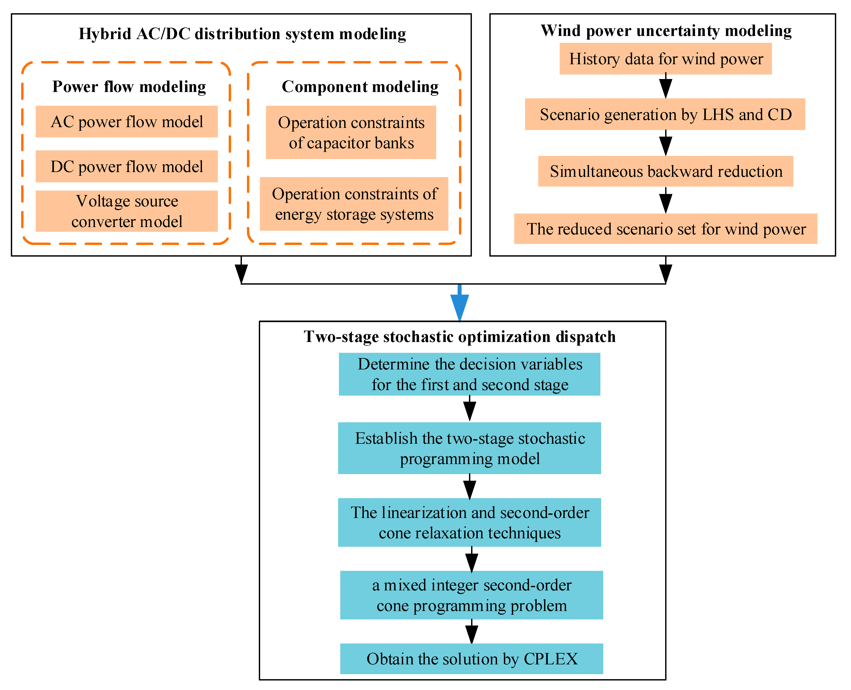
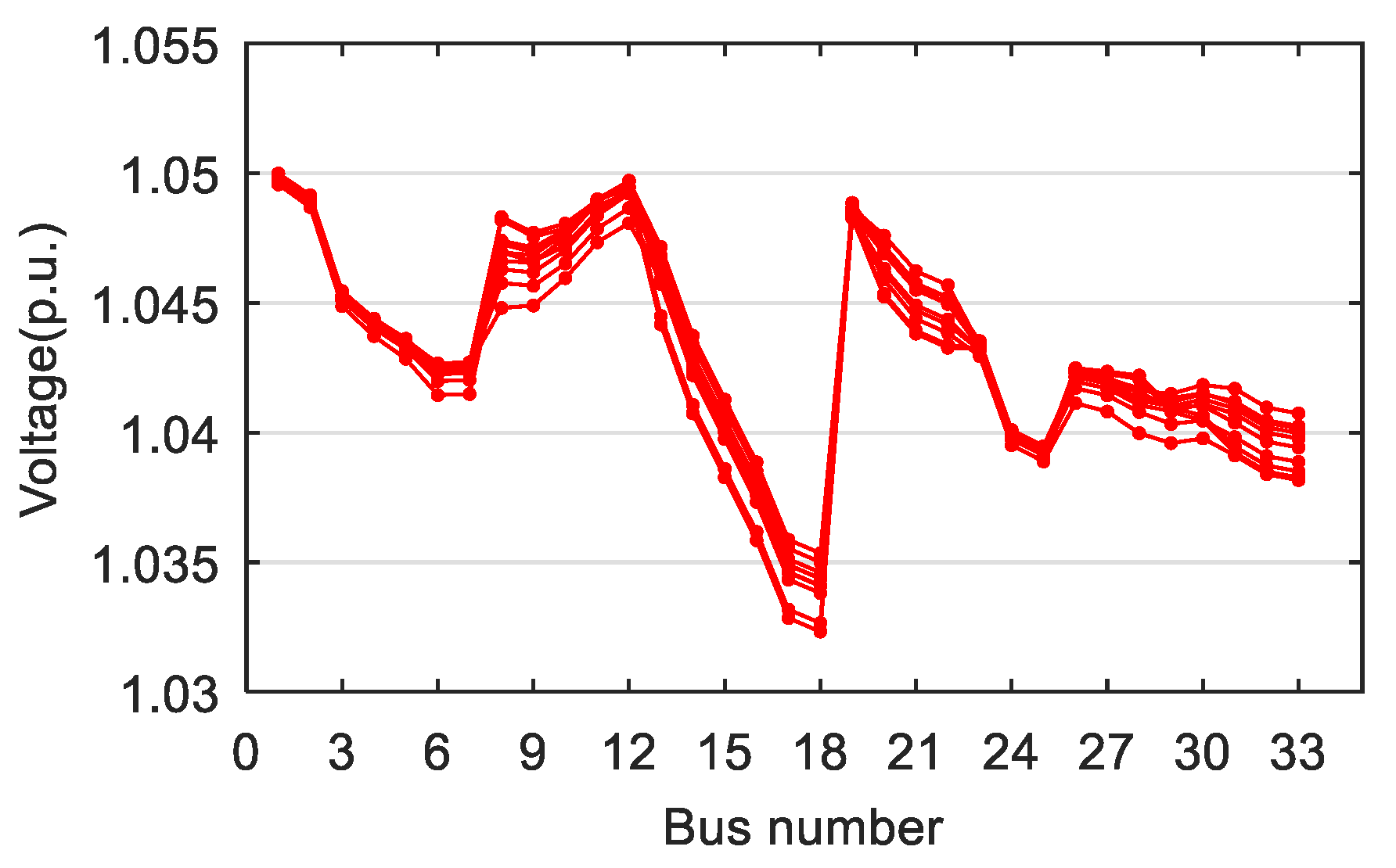
2. Power Flow Model for Hybrid AC/DC Distribution Network

2.1. AC Distribution Network Model

The DistFlow equations are used to describe the power flows in AC distribution system [19]:

$$P_{i,t}^{\mathrm{AC}}={\displaystyle \sum _{k(i,:)\in {ℒ}_{\mathrm{AC}}}{P}_{k,t}^{\mathrm{AC}}}-{\displaystyle \sum _{l(:,i)\in {ℒ}_{\mathrm{AC}}}[P_{l,t}^{\mathrm{AC}}-{(I_{l,t}^{\mathrm{AC}})}^2{r}_l]}\forall i\in {\mathcal{N}}_{\mathrm{AC}},$$

(1)

$$Q_{i,t}^{\mathrm{AC}}={\displaystyle \sum _{k(i,:)\in {ℒ}_{\mathrm{AC}}}{Q}_{k,t}^{\mathrm{AC}}}-{\displaystyle \sum _{l(:,i)\in {ℒ}_{\mathrm{AC}}}[Q_{l,t}^{\mathrm{AC}}-{(I_{l,t}^{\mathrm{AC}})}^2{x}_l]}\forall i\in {\mathcal{N}}_{\mathrm{AC}},$$

(2)

$${(U_{i,t}^{\mathrm{AC}})}^2={(U_{j,t}^{\mathrm{AC}})}^2-2(r_k{P}_{k,t}^{\mathrm{AC}}+x_k{Q}_{k,t}^{\mathrm{AC}})+{(I_{k,t}^{\mathrm{AC}})}^2(r_k^2+x_k^2)\hspace{1em}\forall k(j,i)\in {ℒ}_{\mathrm{AC}},$$

(3)

$${(I_{k,t}^{\mathrm{AC}})}^2{(U_{j,t}^{\mathrm{AC}})}^2={\left(P_{k,t}^{\mathrm{AC}}\right)}^2+{\left(Q_{k,t}^{\mathrm{AC}}\right)}^2\hspace{1em}\forall k(j,i)\in {ℒ}_{\mathrm{AC}},$$

(4)

$${\left(P_{k,t}^{\mathrm{AC}}\right)}^2+{\left(Q_{k,t}^{\mathrm{AC}}\right)}^2\le {(S_{k,\max }^{\mathrm{AC}})}^2\hspace{1em}\forall k(j,i)\in {ℒ}_{\mathrm{AC}},$$

(5)

$$U_{i,\min }^{\mathrm{AC}}\le U_{i,t}^{\mathrm{AC}}\le U_{i,\max }^{\mathrm{AC}}\forall i\in {\mathcal{N}}_{\mathrm{AC}},$$

(6)

where $ℒ$_AC represents the set of AC branches; $𝒩$_AC represents the set of AC nodes; t is the scheduling time; k(i,;) represents branch k starting with node i and l(:,i) represents the branch l ending with node i; r_l and x_l are the resistance and reactance of branch l; $P_{i,t}^{\mathrm{AC}}$ and $Q_{i,t}^{\mathrm{AC}}$ are the injection active and reactive power at node i; $I_{k,t}^{\mathrm{AC}}$, $P_{k,t}^{\mathrm{AC}}$, and $Q_{k,t}^{\mathrm{AC}}$ are the phase current, active, and reactive power at branch k; $U_{j,t}^{\mathrm{AC}}$ and $U_{i,t}^{\mathrm{AC}}$ are the phase voltage at node j and i; $U_{i,\min }^{\mathrm{AC}}$ and $U_{i,\max }^{\mathrm{AC}}$ are the minimum and maximum voltage at node i; and $S_{k,\max }^{\mathrm{AC}}$ is the maximum load flow of AC branch k.

2.2. DC Distribution Network Model

The DC distribution system can be described as:

$$P_{i,t}^{\mathrm{DC}}={\displaystyle \sum _{k(i,:)\in {ℒ}_{\mathrm{DC}}}{P}_{k,t}^{\mathrm{DC}}}-{\displaystyle \sum _{l(:,i)\in {ℒ}_{\mathrm{DC}}}[P_{l,t}^{\mathrm{DC}}-{(I_{l,t}^{\mathrm{DC}})}^2{r}_l]}\forall i\in {\mathcal{N}}_{\mathrm{DC}},$$

(7)

$${(U_{i,t}^{\mathrm{DC}})}^2={(U_{j,t}^{\mathrm{DC}})}^2-2r_k{P}_{k,t}^{\mathrm{DC}}+r_k^2{(I_{k,t}^{\mathrm{DC}})}^2\hspace{1em}\forall k(j,i)\in {ℒ}_{\mathrm{DC}},$$

(8)

$${(I_{k,t}^{\mathrm{DC}})}^2{(U_{j,t}^{\mathrm{DC}})}^2={\left(P_{k,t}^{\mathrm{DC}}\right)}^2\hspace{1em}\forall k(j,i)\in {ℒ}_{\mathrm{DC}},$$

(9)

$$U_{i,\min }^{\mathrm{DC}}\le U_{i,t}^{\mathrm{DC}}\le U_{i,\max }^{\mathrm{DC}}\hspace{1em}\forall i\in {\mathcal{N}}_{\mathrm{DC}},$$

(10)

$$-S_{k,\max }^{\mathrm{DC}}\le P_{k,t}^{\mathrm{DC}}\le S_{k,\max }^{\mathrm{DC}}\hspace{1em}\forall k(j,i)\in {ℒ}_{\mathrm{DC}},$$

(11)

where $ℒ$_DC represents the set of DC branches; $𝒩$_DC represents the set of DC nodes; $P_{i,t}^{\mathrm{DC}}$ is the injection active power at node i; $I_{k,t}^{\mathrm{DC}}$ and $P_{k,t}^{\mathrm{DC}}$ are the phase current and active power at branch k; $U_{i,\min }^{\mathrm{DC}}$ and $U_{i,\max }^{\mathrm{DC}}$ are the minimum and maximum voltage at DC node i; and $S_{k,\max }^{\mathrm{DC}}$ is the maximum load flow of DC branch k.

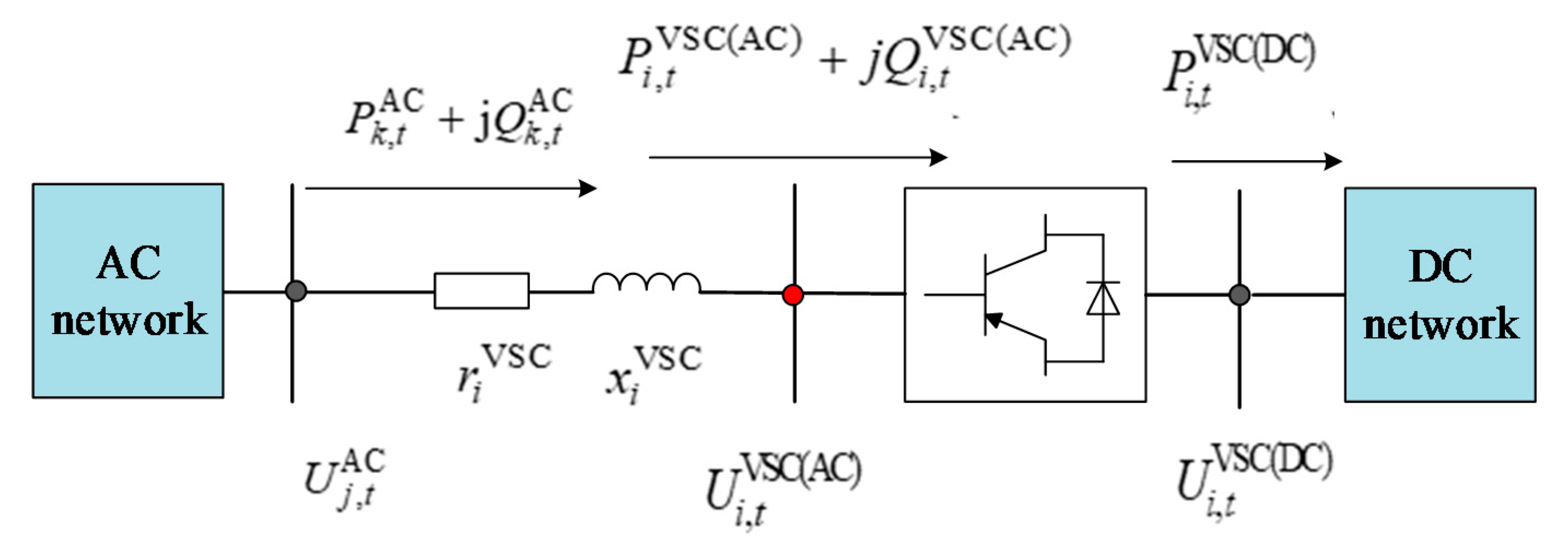
2.3. Voltage Source Converter Model

The schematic diagram of the voltage source converter (VSC) is shown in Figure 2.

As shown in Figure 1, $r_i^{\mathrm{VSC}}$ and $x_i^{\mathrm{VSC}}$ represent the equivalent resistance and reactance of the VSC connected with node j in the AC network. The branch from node j to AC side node i of the VSC can be regarded as the AC branch in the AC network. The VSC model can be described as [20,21]:

$$P_{i,t}^{\mathrm{VSC}\left(\mathrm{AC}\right)}=P_{k,t}^{\mathrm{AC}}-{(I_{k,t}^{\mathrm{AC}})}^2{r}_i^{\mathrm{VSC}}\hspace{1em}\forall i\in {\mathcal{N}}_{\mathrm{SVC}},$$

(12)

$$Q_{i,t}^{\mathrm{SVC}\left(\mathrm{AC}\right)}=Q_{k,t}^{\mathrm{AC}}-{(I_{k,t}^{\mathrm{AC}})}^2{x}_i^{\mathrm{VSC}}\hspace{1em}\forall i\in {\mathcal{N}}_{\mathrm{SVC}},$$

(13)

$${(U_{i,t}^{\mathrm{VSC}\left(\mathrm{AC}\right)})}^2={(U_{j,t}^{\mathrm{AC}})}^2-2(r_i^{\mathrm{VSC}}{P}_{k,t}^{\mathrm{AC}}+x_i^{\mathrm{VSC}}{Q}_{k,t}^{\mathrm{AC}})+{(I_{k,t}^{\mathrm{AC}})}^2[{(r_i^{\mathrm{VSC}})}^2+{(x_i^{\mathrm{VSC}})}^2],$$

(14)

$$3P_{i,t}^{\mathrm{VSC}\left(\mathrm{AC}\right)}=P_{i,t}^{\mathrm{VSC}\left(\mathrm{DC}\right)}\hspace{1em}\forall i\in {\mathcal{N}}_{\mathrm{SVC}},$$

(15)

$$U_{i,t}^{\mathrm{VSC}\left(\mathrm{AC}\right)}=\frac{\sqrt{3}}{3}\mu M_{i,t}{U}_{i,t}^{\mathrm{VSC}\left(\mathrm{DC}\right)}\hspace{1em}\forall i\in {\mathcal{N}}_{\mathrm{SVC}},$$

(16)

where $P_{i,t}^{\mathrm{VSC}\left(\mathrm{AC}\right)}$ and $Q_{i,t}^{\mathrm{SVC}\left(\mathrm{AC}\right)}$ are the input active and reactive power at the AC side of the VSC while $P_{i,t}^{\mathrm{VSC}\left(\mathrm{DC}\right)}$ is the output active power at the DC side of the VSC; $U_{i,t}^{\mathrm{VSC}\left(\mathrm{AC}\right)}$ and $U_{i,t}^{\mathrm{VSC}\left(\mathrm{DC}\right)}$ are the voltage at the AC and DC sides of VSC i; μ is the utilization rate of the DC voltage; and M_i,t is the modulation degree of SVC i within the range of 0 to 1.

2.4. Second-Order Cone Relaxation for the Distribution System Model

For the above model of the hybrid AC/DC distribution network, and the nonlinear terms existing in Equations (1)–(5), (7)–(9), and (12)–(14), the following variables are defined to eliminate the quadratic terms of voltage and current for the AC/DC power flow.

$${(I_{k,t}^{\mathrm{AC}})}^2={\tilde{I}}_{k,t}^{\mathrm{AC}},{(I_{k,t}^{\mathrm{DC}})}^2={\tilde{I}}_{k,t}^{\mathrm{DC}},$$

(17)

$${(U_{i,t}^{\mathrm{AC}})}^2={\tilde{U}}_{i,t}^{\mathrm{AC}},{(U_{i,t}^{\mathrm{DC}})}^2={\tilde{U}}_{i,t}^{\mathrm{DC}}.$$

(18)

Then, Equations (4), (5), and (9) can be converted to second-order cone constraints as follows [22,23]:

$${\Vert {\left[\begin{array}{ccc}2P_{k,t}^{\mathrm{AC}}& 2Q_{k,t}^{\mathrm{AC}}& {\tilde{I}}_{k,t}^{\mathrm{AC}}-{\tilde{U}}_{j,t}^{\mathrm{AC}}\end{array}\right]}^{\mathrm{T}}\Vert }_2\le {\tilde{I}}_{k,t}^{\mathrm{AC}}+{\tilde{U}}_{j,t}^{\mathrm{AC}},$$

(19)

$${\Vert {\left[\begin{array}{cc}{P}_{k,t}^{\mathrm{AC}}& Q_{k,t}^{\mathrm{AC}}\end{array}\right]}^{\mathrm{T}}\Vert }_2\le S_{k,\max }^{\mathrm{AC}},$$

(20)

$${\Vert {\left[\begin{array}{cc}2P_{k,t}^{\mathrm{DC}}& {\tilde{I}}_{k,t}^{\mathrm{DC}}-{\tilde{U}}_{j,t}^{\mathrm{DC}}\end{array}\right]}^{\mathrm{T}}\Vert }_2\le {\tilde{I}}_{k,t}^{\mathrm{DC}}+{\tilde{U}}_{j,t}^{\mathrm{DC}}.$$

(21)

By this means, the hybrid AC/DC distribution system model is transformed as a second-order cone programming problem.

3. Two-Stage Stochastic Scheduling Model for the Hybrid AC/DC Distribution Network

The two-stage stochastic scheduling model is established to cope with wind power uncertainty. The decision at the first stage is applicable for all the wind power scenarios, and the respective adjustment decision for each wind power scenario is made at the second stage.

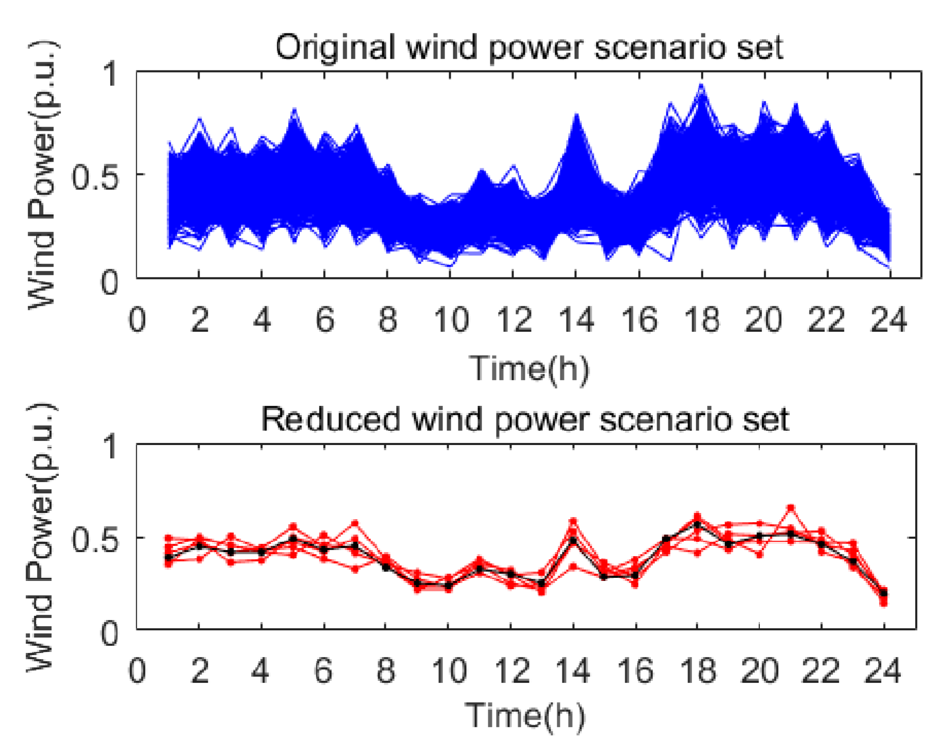
3.1. Scenario Generation and Reduction

The wind power prediction error is regarded as a random variable, which obeys a normal distribution, then the wind power output in real time can be expressed by [24]:

$${\tilde{P}}_t^W={\widehat{P}}_t^W+\Delta {\tilde{P}}_t^W,\Delta {\tilde{P}}_t^W~G(0,{\delta }_t^2),$$

(22)

where $\Delta {\tilde{P}}_t^W$ is the wind power prediction error at time t; ${\widehat{P}}_t^W$ is the day-ahead wind power prediction value; δ_t is the standard deviation of the prediction error; and G represents the normal distribution function.

The scenario generation and reduction techniques are implemented to handle wind power uncertainty. Since the Monte Carlo simulation method based on simple random sampling suffers from a higher computational burden, the Latin hypercube sampling (LHS) is adopted to obtain the original wind power scenario set, which can achieve good coverage from the entire distribution of the random variable [25].

The procedures of LHS can be described as follows:

Step 1: Assuming the number of samples for the random variable, $\Delta {\tilde{P}}_t^W$, is N, the interval [0, 1] can be equally divided into N intervals, and a uniformly distributed random number within the range of [(k−1)/N, k/N] is generated for k = 1 to N;

Step 2: Disorder the order of the above n random numbers obtained by Step 1;

Step 3: The n random numbers by Step 2 are regarded as the probability values of samples, and the value of the random variable, $\Delta {\tilde{P}}_t^W$, can be obtained according to the inverse function of the cumulative distribution function (CDF) for $\Delta {\tilde{P}}_t^W$:

$$\Delta P_t^{(k)}=F_t^{-1}(\frac{k-0.5}{N}),k=1,\cdots ,N,$$

(23)

where F_t(·) represents the CDF of random variable $\Delta {\tilde{P}}_t^W$, and $\Delta P_t^{(k)}$ is the ith sample value of $\Delta {\tilde{P}}_t^W$.

Cholesky decomposition (CD) is introduced to alleviate the undesired correlations between random variables at different time points [26].

The sample matrix for $\Delta {\tilde{P}}_t^W$ by LHS can be expressed as:

$$\Delta \mathit{P}={\left[\begin{array}{cccc}\Delta P_1^{(1)}& \Delta P_1^{(2)}& \cdots & \Delta P_t^{(N)}\\ \Delta P_2^{(1)}& \Delta P_2^{(2)}& \cdots & \Delta P_t^{(N)}\\ ⋮& ⋮& \ddots & ⋮\\ \Delta P_T^{(1)}& \Delta P_T^{(2)}& \cdots & \Delta P_t^{(N)}\end{array}\right]}_{T\times N}.$$

(24)

The procedures of CD are as follows:

Step 1: A T × N ordering matrix, L, is generated, and the element at the tth row and ith column represents the position of the sample, $\Delta P_t^{(k)}$, in the matrix, $\Delta \mathit{P}$, to be arranged;

Step 2: The elements of each row in $\Delta \mathit{P}$ are arranged according to the ordering matrix, L;

Step 3: The corresponding correlation matrix of L noted as ρ_L can be calculated and decomposed by the Cholesky decomposition:

$${\mathbf{\rho }}_L=\mathit{D}{\mathit{D}}^{\mathrm{T}}.$$

(25)

Step 4: A T × N matrix, G, can be obtained by:

$$\mathit{G}={\mathit{D}}^{-1}\mathit{L}.$$

(26)

Step 5: The elements of each row in the matrix, L, are arranged according to the order of elements in the corresponding row in G;

Step 6: The elements of each row in the matrix, $\Delta \mathit{P}$, are arranged according to the updated ordering matrix, L.

Then, the simultaneous backward reduction method is utilized to decrease the number of wind power scenarios [27]. For the matrix, $\Delta \mathit{P}$, obtained by the LHS and CD techniques, the original scenario k noted as $\Delta {\mathit{P}}^{(k)}$ is a vector composed of the elements of the kth row in $\Delta \mathit{P}$, for which the occurrence probability is π^(k). The Kantorovich distance of scenarios $\Delta {\mathit{P}}^{(k)}$ and  $\Delta {\mathit{P}}^{(j)}$ can be defined as:

$$d_{k,j}={\Vert \Delta {\mathit{P}}^{(k)}-\Delta {\mathit{P}}^{(j)}\Vert }_2.$$

(27)

The scenario number in the reduced scenario set is assigned as N_s. The procedures of the simultaneous backward reduction method can be described as follows:

Step 1: Delete the scenario, k, which satisfies the following condition:

$${\pi }^{(k)}{\pi }^{(j)}\underset{k\ne j}{\min }{d}_{k,j}=\underset{m\in \{1,\cdots ,N\}}{\min }{\pi }^{(m)}\left\{\underset{n\in \{1,\cdots ,N\},n\ne m}{\min }{\pi }^{(n)}{d}_{n,m}\right\}.$$

(28)

Step 2: The scenario number is set by N = N − 1, and the scenario, k^*, closest to the deleted scenario, k, is chosen according to:

$$d_{k^{\ast },k}=\underset{s\ne k}{\min }{\pi }^{(k)}{\pi }^{(s)}{d}_{s,k}.$$

(29)

Step 3: The occurrence probability of scenario k^* is set as:

$${\pi }^{(k^{\ast })}={\pi }^{(k^{\ast })}+{\pi }^{(k)}.$$

(30)

Step 4: If N > N_s, return to Step 1; otherwise, the scenario reduction process is finished.

As a result, the reduced scenario set for wind power can be obtained as:

$$\mathcal{P}=\left\{P_{t,s}^W,s=1,2,\cdots ,N_s\right\}.$$

(31)

The parameters, N and N_s, are set to 1000 and 10, respectively. The standard deviation of the wind power prediction error at time point t is set to 20% of ${\widehat{P}}_t^W$. The original and reduced wind power scenario sets are shown in Figure 3.

3.2. Objective Function

The day-ahead scheduling cost includes the generating cost of gas-fired units in the first stage and the power purchasing cost, penalty cost of power fluctuation from the substation, network loss cost, load shedding, and wind curtailment cost:

$$\begin{array}{ll}\min & {\displaystyle \sum _t{\displaystyle \sum _i{c}^G{P}_{i,t}^G}}+{\displaystyle \sum _s{\pi }_s{\displaystyle \sum _t{c}^L({\displaystyle \sum _{i\in {\mathcal{N}}_{\mathrm{AC}}}3}{L}_{i,t,s}^{\mathrm{Cur}}+{\displaystyle \sum _{i\in {\mathcal{N}}_{\mathrm{DC}}}{L}_{i,t,s}^{\mathrm{Cur}}})}}+\\ & {\displaystyle \sum _s{\pi }_s{\displaystyle \sum _t{c}^W({\displaystyle \sum _{i\in {\mathcal{N}}_{\mathrm{AC}}}3}{W}_{i,t,s}^{\mathrm{Cur}}+{\displaystyle \sum _{i\in {\mathcal{N}}_{\mathrm{DC}}}{W}_{i,t,s}^{\mathrm{Cur}}})}}+\\ & {\displaystyle \sum _s{\pi }_s{\displaystyle \sum _t{c}^{\mathrm{Loss}}({\displaystyle \sum _{k\in {ℒ}_{\mathrm{AC}}}3}{(I_{k,t,s}^{\mathrm{AC}})}^2{r}_k+{\displaystyle \sum _{k\in {ℒ}_{\mathrm{DC}}}{(I_{k,t,s}^{\mathrm{DC}})}^2{r}_k})}}+\\ & {\displaystyle \sum _s{\pi }_s{\displaystyle \sum _t{\displaystyle \sum _{i\in {\mathsf{\Omega }}^{\mathrm{Sub}}}(c_t^{\mathrm{Sub}}{P}_{i,t,s}^{\mathrm{Sub}}}+c^{\mathrm{Ramp}}|P_{i,t,s}^{\mathrm{Sub}}-P_{i,t-1,s}^{\mathrm{Sub}}|)}}\end{array}$$

(32)

where c^G is the unit generating cost of gas-fired units; c^L is the load shedding price; c^W is the wind curtailment price; c^Loss is the network loss price; $c_t^{\mathrm{Sub}}$ is the electricity price of the main grid at time t; c^Ramp is the penalty price for power fluctuation; Ω^Sub is the node set of substation; and π_s is the occurrence probability of the wind power scenario, s.

3.3. Constraints for the Two-Stage Stochastic Programming

3.3.1. Operation Constraints of the Capacitor Bank

$$Q_{i,t}^{\mathrm{CB}}=y_{i,t}^{\mathrm{CB}}{Q}_{\mathrm{step}}^{\mathrm{CB}},$$

(33)

$$0\le y_{i,t}^{\mathrm{CB}}\le N_{\max }^{\mathrm{CB}},$$

(34)

$${\displaystyle \sum _t|y_{i,t+1}^{\mathrm{CB}}-y_{i,t}^{\mathrm{CB}}|}\le y_{\max }^{\mathrm{CB}},$$

(35)

where $y_{i,t}^{\mathrm{CB}}$ is the operation number of CB; $N_{\max }^{\mathrm{CB}}$ is the maximum operation number of CB; $Q_{\mathrm{step}}^{\mathrm{CB}}$ is the capacity of single group CB; and $y_{\max }^{\mathrm{CB}}$ is the maximum adjustable number of CB in one day.

It can be seen that the operation number of CB is determined in the first stage, which is applicable for all wind power scenarios in the second stage. In addition, the nonlinear constraint (Equation (35)) can be linearized as follows [28]:

$$\{\begin{array}{l}{y}_{i,t+1}^{\mathrm{CB}}-y_{i,t}^{\mathrm{CB}}\le N_{\max }^{\mathrm{CB}}{b}_t^{\mathrm{CB}}\\ y_{i,t}^{\mathrm{CB}}-y_{i,t+1}^{\mathrm{CB}}\le N_{\max }^{\mathrm{CB}}{b}_t^{\mathrm{CB}}\\ {\displaystyle \sum _t{b}_t^{\mathrm{CB}}}\le y_{\max }^{\mathrm{CB}}\end{array},$$

(36)

where $b_t^{\mathrm{CB}}$ is the binary variable indicating whether the operation number of CB has changed.

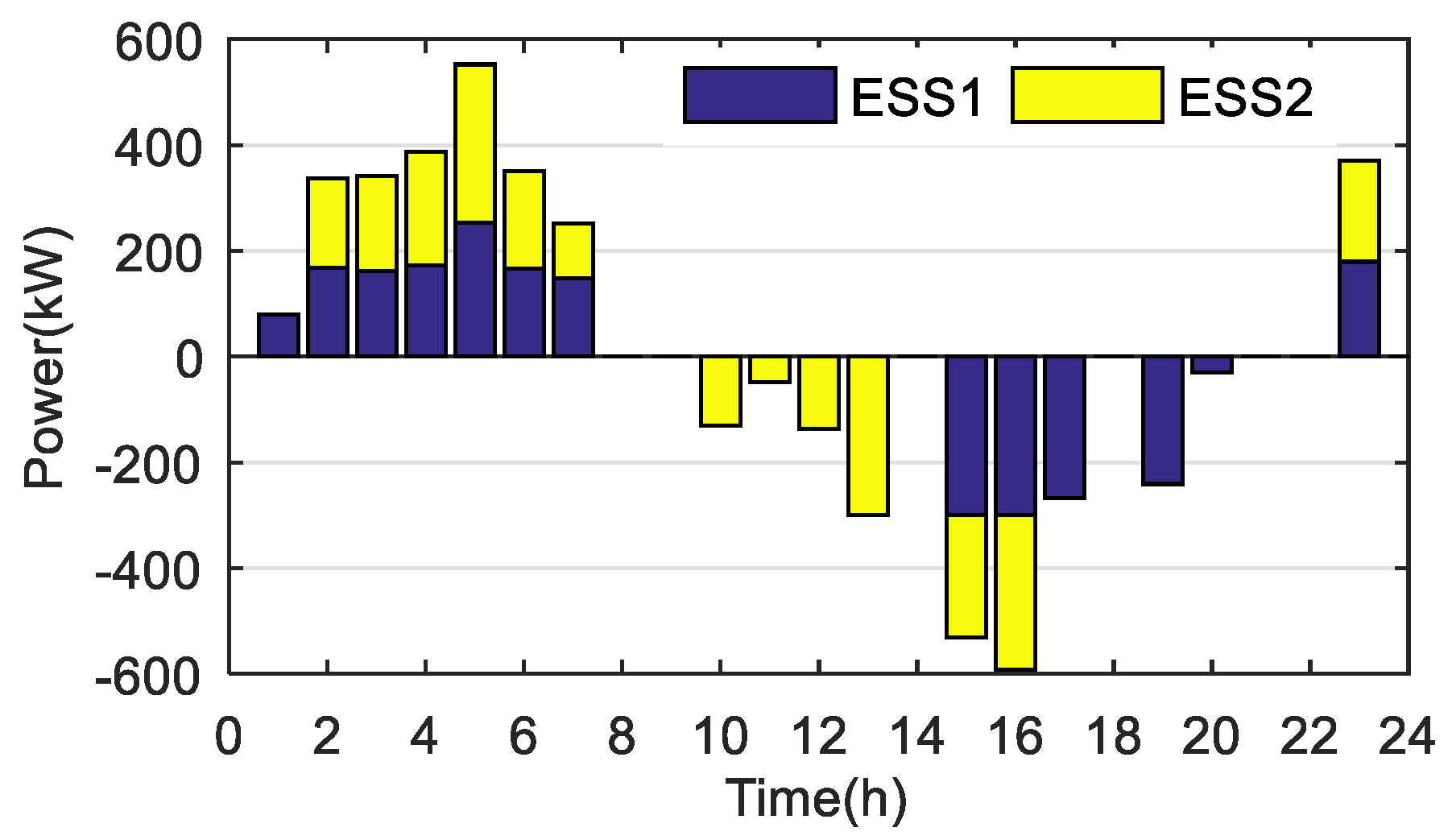
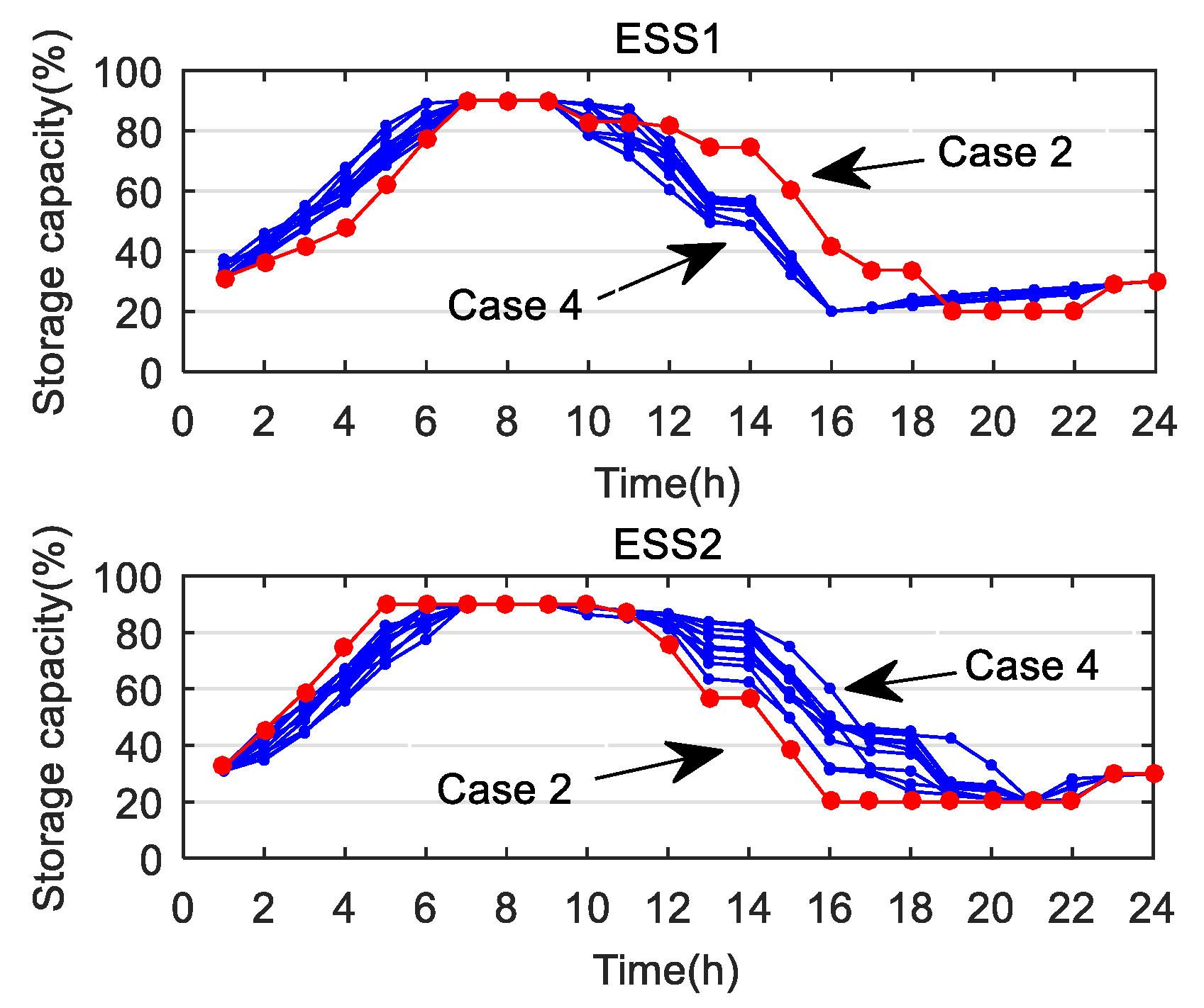
3.3.2. Operation Constraint of the Energy Storage System

$$y_{i,t}^{\mathrm{ch}}+y_{i,t}^{\mathrm{dis}}\le 1,$$

(37)

$$0\le P_{i,t,s}^{\mathrm{dis}}\le y_{i,t}^{\mathrm{dis}}{P}_{\max }^{\mathrm{ESS}},$$

(38)

$$0\le P_{i,t,s}^{\mathrm{ch}}\le y_{i,t}^{\mathrm{ch}}{P}_{\max }^{\mathrm{ESS}},$$

(39)

$$E_{i,t+1,s}^{\mathrm{ESS}}=E_{i,t,s}^{\mathrm{ESS}}+{\eta }^{\mathrm{ch}}{P}_{i,t,s}^{\mathrm{ch}}-{\eta }^{\mathrm{dis}}{P}_{i,t,s}^{\mathrm{dis}},$$

(40)

$$0.2E_{\max }^{\mathrm{ESS}}\le E_{i,t,s}^{\mathrm{ESS}}\le 0.9E_{\max }^{\mathrm{ESS}},$$

(41)

$${\displaystyle \sum _t|y_{i,t+1}^{\mathrm{ch}}-y_{i,t}^{\mathrm{ch}}|}\le y_{\max }^{\mathrm{ESS}},$$

(42)

$${\displaystyle \sum _t|y_{i,t+1}^{\mathrm{dis}}-y_{i,t}^{\mathrm{dis}}|}\le y_{\max }^{\mathrm{ESS}},$$

(43)

where $y_{i,t}^{\mathrm{ch}}$ and $y_{i,t}^{\mathrm{dis}}$ represent the charging and discharging status of the energy storage system; η^ch and η^dis are the charging and discharging efficiency; $P_{\max }^{\mathrm{ESS}}$ is the maximum charging/discharging power; $E_{\max }^{\mathrm{ESS}}$ is the maximum storage capacity; $E_{i,t,s}^{\mathrm{ESS}}$ is the storage capacity of ESS at time t under scenario s; $P_{i,t,s}^{\mathrm{dis}}$ and $P_{i,t,s}^{\mathrm{ch}}$ represent the discharging and charging power output of ESS at time t under scenario s; and $y_{\max }^{\mathrm{ESS}}$ is the maximum charging/discharging number in one day.

It can be seen that the charging/discharging state of ESS noted as $y_{i,t}^{\mathrm{ch}}$ and $y_{i,t}^{\mathrm{dis}}$ is not affected by wind power fluctuations under different scenarios, which remains unchanged during the whole scheduling period. On the other hand, the charging and discharging power output under wind power scenario s are defined as $P_{i,t,s}^{\mathrm{ch}}$ and $P_{i,t,s}^{\mathrm{dis}}$, respectively, which indicates that the charging/discharging power of ESS depends on the possible wind power scenarios. As a result, the charging/discharging state of ESS is regarded as the decision variables in the first stage, which is determined before the possible wind power scenarios happened. Moreover, the charging/discharging power output of ESS is considered as the decision variable in the second stage, which is used to alleviate the wind power fluctuation in real time.

3.3.3. Relevant Constraints of Two Stages

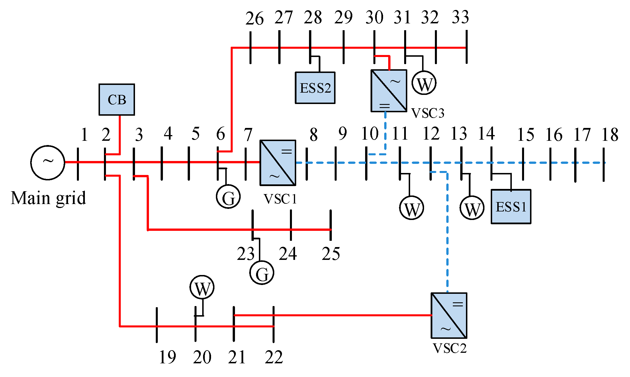
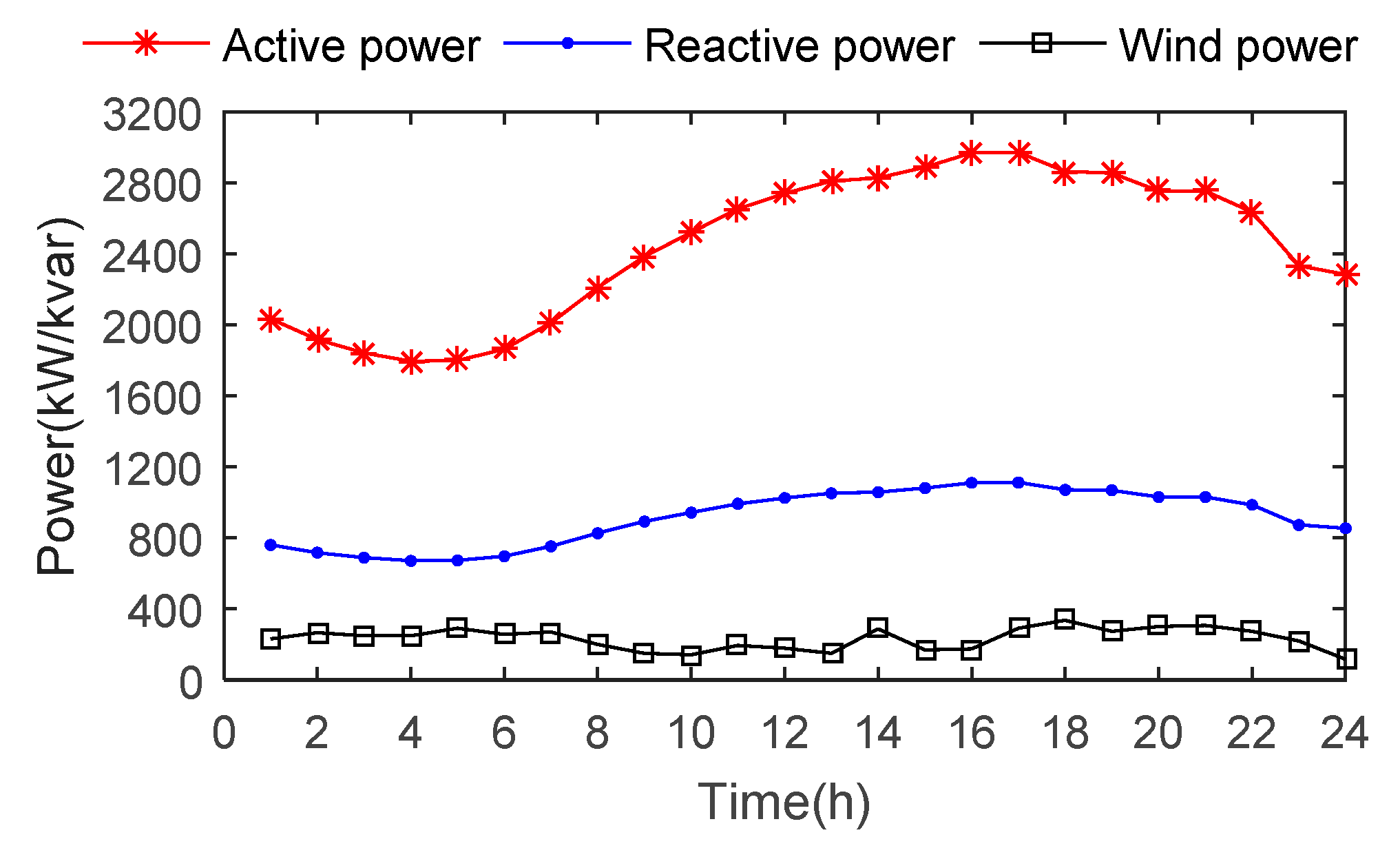
For the two-stage scheduling model, the relevant constraints of the first and second stages are described as follows:

$$P_{i,t,s}^{\mathrm{AC}}=P_{i,t,s}^{\mathrm{Sub}}+P_{i,t,s}^W+P_{i,t}^G+P_{i,t,s}^{\mathrm{dis}}-P_{i,t,s}^{\mathrm{ch}}-P_{i,t}^L\hspace{1em}\forall i\in {\mathcal{N}}_{\mathrm{AC}},$$

(44)

$$Q_{i,t,s}^{\mathrm{AC}}=Q_{i,t,s}^{\mathrm{Sub}}+Q_{i,t,s}^W+Q_{i,t}^G+Q_{i,t}^{\mathrm{CB}}-Q_{i,t}^L\hspace{1em}\forall i\in {\mathcal{N}}_{\mathrm{AC}},$$

(45)

$$P_{i,t}^{\mathrm{DC}}=P_{i,t,s}^W+P_{i,t,s}^{\mathrm{VSC}(\mathrm{DC})}-P_{i,t}^L\hspace{1em}\forall i\in {\mathcal{N}}_{\mathrm{DC}},$$

(46)

where $P_{i,t,s}^{\mathrm{Sub}}$ and $Q_{i,t,s}^{\mathrm{Sub}}$ represent the active and reactive power from the substation connected with node i at time t under scenario s; $P_{i,t,s}^W$ and $Q_{i,t,s}^W$ represent the active and reactive power from the wind generator under scenario s; $P_{i,t}^G$ and $Q_{i,t}^G$ represent the active and reactive power output by the gas-fired units; and $P_{i,t}^L$ and $Q_{i,t}^L$ represent the active and reactive power load at node i.

In this study, the gas consumption plan by gas-fired units is determined before wind power uncertainty is observed and will not adjust in real time. Consequently, the power output of gas-fired units cannot be changed under different wind power scenarios at the second stage.

Furthermore, the hybrid AC/DC distribution network model in Section 2 is established for the certain wind power scenario. In other words, all the variables in Equations (1)–(21) should be changed to the corresponding variables for different wind power scenarios. Taking the DC distribution network as an example, $U_{i,t}^{\mathrm{DC}}$, $I_{k,t}^{\mathrm{DC}}$, and $P_{k,t}^{\mathrm{DC}}$ should be replaced by $U_{i,t,s}^{\mathrm{DC}}$, $I_{k,t,s}^{\mathrm{DC}}$, and $P_{k,t,s}^{\mathrm{DC}}$, respectively. Additionally, the power flow model for the DC distribution network under scenario s can be expressed as follows:

$$\{\begin{array}{l}{P}_{i,t,s}^{\mathrm{DC}}={\displaystyle \sum _{k(i,:)\in {ℒ}_{\mathrm{DC}}}{P}_{k,t,s}^{\mathrm{DC}}}-{\displaystyle \sum _{l(:,i)\in {ℒ}_{\mathrm{DC}}}(P_{l,t,s}^{\mathrm{DC}}-{\tilde{I}}_{l,t,s}^{\mathrm{DC}}{r}_l)}\forall i\in {\mathcal{N}}_{\mathrm{DC}}\\ {\tilde{U}}_{i,t,s}^{\mathrm{DC}}={\tilde{U}}_{j,t,s}^{\mathrm{DC}}-2r_k{P}_{k,t,s}^{\mathrm{DC}}+{\tilde{I}}_{k,t,s}^{\mathrm{DC}}{r}_k^2\hspace{1em}\forall k(j,i)\in {ℒ}_{\mathrm{DC}}\\ {\Vert {\left[\begin{array}{cc}2P_{k,t,s}^{\mathrm{DC}}& {\tilde{I}}_{k,t,s}^{\mathrm{DC}}-{\tilde{U}}_{j,t,s}^{\mathrm{DC}}\end{array}\right]}^{\mathrm{T}}\Vert }_2\le {\tilde{I}}_{k,t,s}^{\mathrm{DC}}+{\tilde{U}}_{j,t,s}^{\mathrm{DC}}\\ {(U_{i,\min }^{\mathrm{DC}})}^2\le {\tilde{U}}_{i,t,s}^{\mathrm{DC}}\le {(U_{i,\max }^{\mathrm{DC}})}^2\forall i\in {\mathcal{N}}_{\mathrm{DC}}\\ -S_{k,\max }^{\mathrm{DC}}\le P_{k,t,s}^{\mathrm{DC}}\le S_{k,\max }^{\mathrm{DC}}\hspace{1em}\forall k(j,i)\in {ℒ}_{\mathrm{DC}}\end{array}.$$

(47)

The power flow model for the AC distribution network and VSC under the wind power scenario, s, can be expressed in a similar way, but the corresponding formulas are not listed here to save page.

4. Case Studies

The case study was conducted based on the modified IEEE 33-node hybrid AC/DC distribution system [19]. As shown in Figure 4, the solid red lines represent AC branches and the dashed blue lines represent DC branches. The rated voltages of the AC and DC distribution network are 12.66 and 15 kV, respectively. The voltage limitation range was set to [0.95, 1.05] p.u. There are two gas-fired units with the capacity of 300 kW, and three VSCs and four wind generators with the capacity of 500 kW in the hybrid system. The electricity price of main grid is 0.12 $/kWh at hour 7–22 and 0.06 $/kWh at other times. The operation parameters of different facilities and the cost coefficients are listed in

Table 1. Parameters of capacitor bank.

Bus Node	${\mathit{Q}}_{\mathbf{s}\mathbf{t}\mathbf{e}\mathbf{p}}^{\mathbf{C}\mathbf{B}}$/kVar	${\mathit{N}}_{\mathbf{m}\mathbf{a}\mathbf{x}}^{\mathbf{C}\mathbf{B}}$	${\mathit{y}}_{\mathbf{m}\mathbf{a}\mathbf{x}}^{\mathbf{C}\mathbf{B}}$
2	60	5	3

,

Table 2. Parameters ofenergy storage system.

Bus Node	${\mathit{P}}_{\mathbf{m}\mathbf{a}\mathbf{x}}^{\mathbf{E}\mathbf{S}\mathbf{S}}$/kW	${\mathit{E}}_{\mathbf{m}\mathbf{a}\mathbf{x}}^{\mathbf{E}\mathbf{S}\mathbf{S}}$/(kWh)	${\mathit{E}}_{\mathbf{i}\mathbf{n}\mathbf{t}}^{\mathbf{E}\mathbf{S}\mathbf{S}}$/%	ηch	ηdis	${\mathit{y}}_{\mathbf{m}\mathbf{a}\mathbf{x}}^{\mathbf{E}\mathbf{S}\mathbf{S}}$
14, 28	300	1800	30	0.9381	1.1066	3

,

Table 3. Parameters ofvoltage source converter.

Bus Node	${\mathit{Q}}_{\mathbf{m}\mathbf{a}\mathbf{x}}^{\mathbf{S}\mathbf{V}\mathbf{C}\left(\mathbf{A}\mathbf{C}\right)}$/kVar	${\mathit{S}}_{\mathbf{m}\mathbf{a}\mathbf{x}}^{\mathbf{S}\mathbf{V}\mathbf{C}\left(\mathbf{A}\mathbf{C}\right)}$/kVA	μ
7, 21, 30	600	1500	0.866

,

Table 4. Parameters of gas-fired units.

Bus Node	${\mathit{P}}_{\mathbf{m}\mathbf{i}\mathbf{n}}^{\mathit{G}}$/kW	${\mathit{P}}_{\mathbf{m}\mathbf{a}\mathbf{x}}^{\mathit{G}}$/kW	${\mathit{Q}}_{\mathbf{m}\mathbf{a}\mathbf{x}}^{\mathit{G}}$/kW
6, 23	30	300	150

and

Table 5. Parameters for cost.

Parameters	cG	cL	cW	cLoss	cRamp
values/($/kWh)	0.042	1	0.2	0.032	0.04

. The unit generating cost of gas-fired units and power fluctuation cost in Table 5 were obtained from [29], the unit network loss cost was obtained from [21], and the unit penalty costs for wind curtailment and load shedding can be found in [30]. The load demand and wind power curves are shown in Figure 5. The power output predictions of four wind generators are the same, and the wind generators in the AC distribution network are running at a constant power factor of 0.85. In this study, the solving tool Yalmip was adopted to develop the above application programs and then solved by Cplex in the MATLAB platform [31].

The following cases were considered to demonstrate the effectiveness of proposed model:

Case 1:

Day-ahead scheduling for the hybrid distribution system with CB considering the wind power prediction curve;

Case 2:

Day-ahead scheduling for the hybrid distribution system with CB and ESS considering the wind power prediction curve;

Case 3:

Two-stage stochastic scheduling for the hybrid distribution system with CB considering th wind power scenario set; and

Case 4:

Two-stage stochastic scheduling for the hybrid distribution system with CB and ESS considering the wind power scenario set.

The simulation results for the above cases are listed in

Table 6. Simulation results for different cases.

Case	Power Purchasing Cost ($)	Power Fluctuation Penalty Cost ($)	Power Loss (kW)	Load Shedding(kW)
Case 1	2463.86	178.81	186.47	0
Case 2	2343.83	57.95	181.62	0
Case 3	2487.71	240.71	225.78	0
Case 4	2427.25	75.05	203.12	0

. When the active and reactive power load at all the nodes were increased by 12.5%, the simulation results for the above four cases are listed in

Table 7. Simulation results for different cases.

Case	Power Purchasing Cost ($)	Power Fluctuation Penalty Cost ($)	Power Loss (kW)	Load Shedding(kW)
Case 1	3230.61	178.56	273.38	62.23
Case 2	3118.27	52.73	268.27	0
Case 3	3249.85	235.76	319.21	110.34
Case 4	3134.96	80.01	276.65	0

.

From Table 6, it can be seen that: (1) The power loss cost, the power purchasing cost, and power fluctuation penalty costs of the main grid in Case 2 were reduced prominently compared to Case 1, and a similar situation occurs between Case 3 and Case 4, which indicates that considering ESSs can improve the economical performance of the dispatch solution; (2) the various costs in Case 1 are less than the corresponding values in Case 3, and a similar situation exists between Cases 2 and 4. Yet, the deterministic scheduling model is adopted in Cases 1 and 2 while the two-stage stochastic scheduling model is implemented in Cases 3 and 4. Apparently, wind power uncertainty is not taken into consideration in the deterministic scheduling model, which is inconsistent with the actual situation. By contrast, the wind power scenario set has been introduced by the proposed model in Cases 3 and 4 to describe wind power fluctuation in real time. In other words, the influence of wind power uncertainty on the dispatch solution is integrated into the decision process. As a result, the two-stage stochastic scheduling model has increased the operation cost compared with the deterministic scheduling model, but the reliability of the dispatch solution has been improved.

From Table 7, it can be found that load shedding happened in Cases 1 and 3 with the increase of the active and reactive power load, in which ESSs are not integrated in the hybrid AC/DC distribution network. Considering ESSs in Cases 2 and 4 can prominently enhance the economy and reliability of system operation compared with Cases 1 and 3.

Furthermore, the operation status of regulating facilities, such as VSC and ESS, is investigated as follows. For the deterministic scheduling model in Case 2, the transferred active/reactive power by the VSC facilities and the charging/discharging power by ESS are shown in Figure 6 and Figure 7, respectively. It can be seen that: (1) VSC3 operates under the working mode of inverting while VSC1 and VSC2 operate under the working mode of rectifying; (2) as shown in Figure 7, the positive values of power denote that ESS works in the charging state and the negative values mean it works in the discharging state. Combined with the load curves in Figure 5, during the load valley periods of 1 to 8, ESS stored the surplus energy generated by wind generators and the main grid. During the load increasing period of 10 to 20, ESS discharged the previous stored energy to satisfy the balance of supply and demand. By this means, the power fluctuation of the main grid can be alleviated. Meanwhile, ESS can store energy when the electricity price is lower and discharge energy when the electricity price is higher to reduce the power purchasing cost from the main grid.

For the two-stage stochastic scheduling model in Case 4, the transferred active and reactive power by the VSC facilities under different scenarios are shown in Figure 8, and the voltage profiles under different wind power scenarios at hour 17 are shown in Figure 9. From Figure 8, it can be seen that the deviation of transferred power by VSC1 among different wind power scenarios is less than that by VSC2 and VSC3. The reason is that the location nodes of VSC2 and VSC3 are very close to wind generators, the power uncertainty of which has a direct impact on the transmission power of VSC. Combining Figure 8 and Figure 9, it can be found that the node 12 has the highest voltage value for the DC nodes from 8 to 18. The reason is that during the whole scheduling period, SVC2 transferred a large amount of active power to the DC distribution network through node 12, which can be regarded as the DC power supply.

Furthermore, the storage capacity curves by ESS in Cases 2 and 4 when the power load increased by 12.5% are shown in Figure 10. It can be seen that: (1) For the two-stage stochastic scheduling model in Case 4, the charging and discharging periods of ESS are consistent during the whole scheduling period while the charging and discharging power changed with different wind power scenarios; and (2) the charging/discharging period of ESS1 and ESS2 for the deterministic scheduling model in Case 2 is shorter compared to that in Case 4. For instance, ESS1 is not in use at hours 19 to 22 and ESS2 is not in use at hours 16 to 20 in Case 2 while the above ESSs are in the discharging/charging mode at these hours.

In addition, to verify the performance of the proposed model, the charging/discharging state of ESSs obtained by the deterministic scheduling model in Case 2 is implemented for the two-stage stochastic scheduling model in Case 4. The simulated results indicate that the power purchasing cost and power loss cost are similar to the corresponding values while the power fluctuation penalty cost has increased by $36.56 compared to the corresponding value shown in Table 7. It can be drawn that for the same charging/discharging state of ESSs, the two-stage stochastic scheduling model can make more economic decisions to reduce the power fluctuation penalty cost. On the other hand, the scheduling solution by the two-stage stochastic scheduling model has greater decision reliability under the consideration of different wind power scenarios in real time. As a result, the scheduling strategy achieved by the proposed model shows superior performance to ensure the economic and stable operation of the hybrid AC/DC distribution system considering wind power uncertainty.

5. Conclusions

This paper proposed a two-stage stochastic scheduling model for the hybrid AC/DC distribution system considering wind power uncertainty. With the purpose of achieving the active-reactive power coordinated optimal dispatch, the capacitor bank, energy storage system, and voltage source converter were introduced as the active adjustment measures. By using the linearization and second-order cone relaxation techniques for the above distribution network model, the original nonlinear optimization problem could be transformed into a mixed integer second-order cone programming problem to solve. Then, the modified IEEE 33-node hybrid AC/DC distribution system was employed to verify the performance of the proposed model. Th simulation results demonstrated that the two-stage stochastic scheduling model can achieve effective decision-making to ensure the economic and stable operation of the hybrid AC/DC distribution system with wind power integration.

References

1. Zhao, B.; Zhao, Y.; Wang, Y.; Liu, G.; Song, Q.; Yuan, Z.; Yao, S. Energy internet system based on flexible medium-voltage DC distribution. Proc. CSEE 2015, 35, 4834–4851. [Google Scholar]
2. Salomonsson, D.; Sannino, A. Low-voltage DC distribution system for commercial power systems with sensitive electronic loads. IEEE Trans. Power Deliv. 2007, 22, 1620–1627. [Google Scholar] [CrossRef]
3. Starke, M.; Li, F.; Tolbert, L.M.; Ozpineci, B. AC vs. DC distribution: Maximum transfer capability. In Proceedings of the 2008 IEEE Power and Energy Society General Meeting—Conversion and Delivery of Electrical Energy in the 21st Century, 20–24 July 2008; IEEE: Pittsburgh, PA, USA, 2008. [Google Scholar]
4. Wang, P.; Goel, L.; Liu, X.; Choo, F.H. Harmonizing AC and DC: A hybrid AC/DC future grid solution. IEEE Power Energy Mag. 2013, 11, 76–83. [Google Scholar] [CrossRef]
5. Eajal, A.A.; Shaaban, M.F.; Ponnambalam, K.; El-Saadany, E.F. Stochastic centralized dispatch scheme for AC/DC hybrid smart distribution systems. IEEE Trans. Sustain. Energy 2017, 7, 1046–1059. [Google Scholar] [CrossRef]
6. Ahmed, H.M.A.; Eltantawy, A.B.; Salama, M.M.A. A generalized approach to the load flow analysis of AC–DC hybrid distribution systems. IEEE Trans. Power Syst. 2018, 33, 2117–2127. [Google Scholar] [CrossRef]
7. Chaudhary, S.K.; Guerrero, J.M.; Teodorescu, R. Enhancing the capacity of the AC distribution system using DC interlinks-a step toward future DC grid. IEEE Trans. Smart Grid 2015, 6, 1722–1729. [Google Scholar] [CrossRef]
8. Xu, Y.; Dong, Z.; Zhang, R.; Hill, D.J. Multi-timescale coordinated voltage/var control of high renewable-penetrated distribution systems. IEEE Trans. Power Syst. 2017, 32, 4398–4408. [Google Scholar] [CrossRef]
9. Zhang, L.; Tang, W.; Liang, J.; Cong, P.; Cai, Y. Coordinated day-ahead reactive power dispatch in distribution network based on real power forecast errors. IEEE Trans. Power Syst. 2015, 31, 2472–2480. [Google Scholar] [CrossRef]
10. Zhang, L.; Tang, W.; Liang, J.; Li, G.; Cai, Y.; Yan, T. A medium voltage hybrid AC/DC distribution network and its economic evaluation. In Proceedings of the 12nd IET International Conference on AC and DC Power Transmission, Beijing, China, 28–29 May 2016. [Google Scholar]
11. Zhang, L.; Chen, Y.; Shen, C.; Tang, W.; Jun, L. Coordinated voltage regulation of hybrid AC/DC medium voltage distribution networks. J. Mod. Power Syst. Clean Energy 2018, 6, 463–472. [Google Scholar] [CrossRef] [Green Version]
12. Wang, L.; Liang, D.H.; Crossland, A.F.; Taylor, P.C.; Jones, D.; Wade, N.S. Coordination of multiple energy storage units in a low-voltage distribution network. IEEE Trans. Smart Grid 2015, 6, 2906–2918. [Google Scholar] [CrossRef] [Green Version]
13. Li, X.; Yao, L.; Hui, D. Optimal control and management of a large-scale battery energy storage system to mitigate fluctuation and intermittence of renewable generations. J. Mod. Power Syst. Clean Energy 2016, 4, 593–603. [Google Scholar] [CrossRef] [Green Version]
14. Mahdavi, S.; Hemmati, R.; Jirdehi, M.A.; Department of Electrical Engineering, Kermanshah University of Technology. Two-level planning for coordination of energy storage systems and wind-solar-diesel units in active distribution networks. Energy 2018, 151, 954–965. [Google Scholar] [CrossRef]
15. Zheng, Y.; Zhao, J.; Song, Y.; Luo, F.; Meng, K.; Qiu, J.; Hill, D.J. Optimal operation of battery energy storage system considering distribution system uncertainty. IEEE Trans. Sustain. Energy 2018, 9, 1051–1060. [Google Scholar] [CrossRef]
16. Kazari, H.; Oraee, H.; Pal, B.C. Assessing the Effect of Wind Farm Layout on Energy Storage Requirement for Power Fluctuation Mitigation. IEEE Trans. Sustain. Energy 2019, 10, 558–568. [Google Scholar] [CrossRef]
17. Li, Y.; Wang, J.; Gu, C.; Liu, J.; Li, Z. Investment optimization of grid-scale energy storage for supporting different wind power utilization levels. J. Mod. Power Syst. Clean Energy 2019, 7, 1721–1734. [Google Scholar] [CrossRef] [Green Version]
18. Tomczewski, A.; Kasprzyk, L. Optimisation of the structure of a wind farm—Kinetic energy storage for improving the reliability of electricity supplies. Appl. Sci. 2018, 8, 1439. [Google Scholar] [CrossRef] [Green Version]
19. Baran, M.E.; Wu, F.F. Network reconfiguration in distribution systems for loss reduction and load balancing. IEEE Trans. Power Deliv. 1989, 4, 1401–1407. [Google Scholar] [CrossRef]
20. Wang, S.; Chen, S.; Xie, S. Security-constrained coordinated economic dispatch of energy storage systems and converter stations for AC/DC distribution networks. Autom. Electr. Power Syst. 2017, 41, 85–91. [Google Scholar]
21. Ma, X.; Guo, R.; Wang, L.; Huang, J.; Liu, J.; Fang, C. Day-ahead scheduling model for AC/DC active distribution network based on second-order cone programming. Autom. Electr. Power Syst. 2018, 42, 144–150. [Google Scholar]
22. Farivar, M.; Low, S.H. Branch flow model: Relaxations and convexification—Part I. IEEE Trans. Power Syst. 2013, 28, 2554–2564. [Google Scholar] [CrossRef]
23. Low, S.H. Convex relaxation of optimal power flow, Part II: Exactness. IEEE Trans. Control. Netw. 2014, 1, 177–189. [Google Scholar] [CrossRef] [Green Version]
24. Zhang, Y.; Liu, K.; Liao, X.; Qin, L.; An, X. Stochastic dynamic economic emission dispatch with unit commitment problem considering wind power integration. Int. Trans. Electr. Energy 2017, 28, e2472. [Google Scholar] [CrossRef]
25. Mckay, M.D.; Beckman, R.J.; Conover, W.J. A comparison of three methods for selecting values of input variables in the analysis of output from a computer code. Technometrics 1979, 21, 239–245. [Google Scholar]
26. Harbrecht, H.; Peters, M.; Schneider, R. On the low-rank approximation by the pivoted Cholesky decomposition. Appl. Numer. Math. 2012, 62, 428–440. [Google Scholar] [CrossRef] [Green Version]
27. Wu, L.; Shahidehpour, M.; Li, T. Stochastic security-constrained unit commitment. IEEE Trans. Power Syst. 2007, 22, 800–811. [Google Scholar] [CrossRef]
28. Gao, H.; Wang, L.; Liu, J.; Wei, Z. Integrated day-ahead scheduling considering active management in future smart distribution system. IEEE Trans. Power Syst. 2018, 33, 6049–6061. [Google Scholar] [CrossRef]
29. Wang, J.; Xu, J.; Liao, S.; Sima, L.; Sun, Y.; Wei, C. Coordinated optimization of integrated electricity-gas energy system considering uncertainty of renewable energy output. Autom. Electr. Power Syst. 2019, 43, 2–9. [Google Scholar]
30. Zhang, Y.; Le, J.; Zheng, F.; Liu, K. Two-stage distributionally robust coordinated scheduling for gas-electricity integrated energy system considering wind power uncertainty and reserve capacity configuration. Renew. Energy 2019, 135, 122–135. [Google Scholar] [CrossRef]
31. Lofberg, J. YALMIP: A toolbox for modeling and optimization in MATLAB. In Proceedings of the 2004 IEEE International Symposium on Computer Aided Control Systems Design, Taipei, China, 2–4 September 2004; pp. 284–289. [Google Scholar]
Figure 1. The schematic framework of this study.
Applsci 10 00181 g001
Figure 2. Schematic diagram of the voltage source converter.
Applsci 10 00181 g002
Figure 3. The original and reduced wind power scenario sets.
Applsci 10 00181 g003
Figure 4. The modified IEEE 33-node hybrid AC/DC distribution network.
Applsci 10 00181 g004
Figure 5. Wind power output and load curves.
Applsci 10 00181 g005
Figure 6. The transferred active and reactive power by VSC in Case 2.
Applsci 10 00181 g006
Figure 7. The charging/discharging power of energy storage system in Case 2.
Applsci 10 00181 g007
Figure 8. The transferred active and reactive power by voltage source converter in Case 4.
Applsci 10 00181 g008
Figure 9. Voltage profiles at hour 17 in Case 4.
Applsci 10 00181 g009
Figure 10. Storage capacity of ESS in Cases 2 and 4.
Applsci 10 00181 g010