Prediction of Friction Resistance for Slurry Pipe Jacking

Featured Application

The new approach established in this paper can provide accuracy prediction of friction resistance for slurry pipe jacking with various soil conditions, which lays a good foundation for better future design and less construction costs.

Abstract

Friction resistance usually constitutes one of the two main components for the calculation of required jacking force. This paper provides a new approach to predict the friction resistance of slurry pipe jacking. First, the existing prediction equations and their establishment methods and essential hypotheses used were carefully summarized and compared, providing good foundations for the establishment of the new model. It was found that the friction resistance can be uniformly calculated by multiplying an effective friction coefficient and the normal force acting on the external surface of the pipe. This effective friction coefficient is introduced to reflect the effect of contact state of pipe-soil-slurry, highly affected by the effect of lubrication and the interaction of pipe-soil-slurry. The critical quantity of pipe-soil contact angle (or width) involved may be calculated by Persson’s contact model. Then, the equation of normal force was rederived and determined, in which the vertical soil stress should be calculated by Terzaghi’s silo model with parameters proposed by the UK Pipe Jacking Association. Different from the existing prediction models, this new approach has taken into full consideration the effect of lubrication, soil properties (such as internal friction angle, cohesion, and void ratio), and design parameters (such as buried depth, overcut, and pipe diameter). In addition, four field cases and a numerical simulation case with various soils and design parameters were carefully selected to check out the capability of the new model. There was greater satisfaction with the measured data as compared to the existing models and the numerical simulation approach, indicating that the new approach not only has higher accuracy but is also more flexible and has a wider applicability. Finally, the influence of buried depth, overcut, and pipe diameter on the friction resistance and lubrication efficiency were analyzed, and the results can be helpful for the future design.

1. Introduction

In many parts of the world, the numerous constructions of municipal tunnels are creating unforeseen problems, such as blocking of roads, existing pipelines failure, and buildings subsidence. This has motivated attempts at the development of trenchless construction technology, such as pipe jacking, especially in metropolitan cities [1,2]. Pipe jacking is defined as a trenchless excavation technique, which employs hydraulic jacks to thrust specially made pipes through the ground behind a jacking machine, from a drive shaft to a reception shaft, as illustrated in Figure 1. It has many technical merits, such as a short time limit, high security, low environmental effect, and little traffic disturbance [3,4,5,6]. Because of that, pipe jacking has been widely used in the construction of infrastructure for traffic and transportation systems in cities [7,8].

In pipe jacking, the jacking force is a critical factor that determines the thickness of pipe and reaction wall, selection or design of jacking machine and lubricant requirements [9]. The accuracy of prediction of jacking force is directly related to the structural safety and construction cost.

The main component of the jacking force is due to frictional resistance. Application of a lubricant such as bentonite slurry in pipe jacking (so-called ‘slurry pipe jacking’) is essential to reduce the friction resistance and, therefore, the jacking force [3,10,11,12,13]. However, the use of slurry makes it more complex to calculate or predict the friction resistance because of the change in contact conditions between the pipe and soil and lubricant slurry. The new contact state, which is due to the pipe-soil-slurry interaction, is affected by factors such as pipe diameter, soil properties, overcut [3,9], lubrication efficiency [9], pipeline misalignments [10,14,15,16], and stoppages [9,14,17,18,19]. The existing prediction models have not fully taken these factors into consideration, leading to an overestimation or underestimation of the friction resistance [9,20,21,22,23]. It is therefore obvious that a new prediction approach or model is imperatively needed to be established to solve the problem in slurry pipe jacking [24].

2. Overview of the Existing Prediction Models of Friction Resistance

Numerous models that calculate the friction resistance of pipe jacking have been proposed by authors from all over the world. The superposition principle is usually used, which holds that the comprehensive outcome of two or more linear factors of a system is equal to the accumulation of the effect of each factor. In pipe jacking, the linear factors to generate friction resistance are due to the weight of pipe (f_W), soil pressure (f_s), slurry pressure (f_m), pipe-soil cohesion (f_sc), and pipe-slurry cohesion (f_mc). Their equations can be expressed as [5,6,9,10,14,19,21,22,25,26].

$$f_W={\mu }_{s}W$$

(1)

$$f_s={\mu }_{s}N$$

(2)

$$f_m={\mu }_{m}N$$

(3)

$$f_{sc}=c_s{B}_s$$

(4)

$$f_{mc}=c_m{B}_m$$

(5)

where μ_s and μ_m are the kinematic friction coefficient of pipe-soil and pipe-slurry, respectively; W is the weight of pipe per unit length, kN/m; N is the total normal force acting on the pipe, kN/m; c_s and c_m are the pipe-soil cohesion resistance and pipe-slurry cohesion resistance, respectively, kPa; B_s and B_m are the pipe-soil contact width and pipe-slurry contact width, respectively, m.

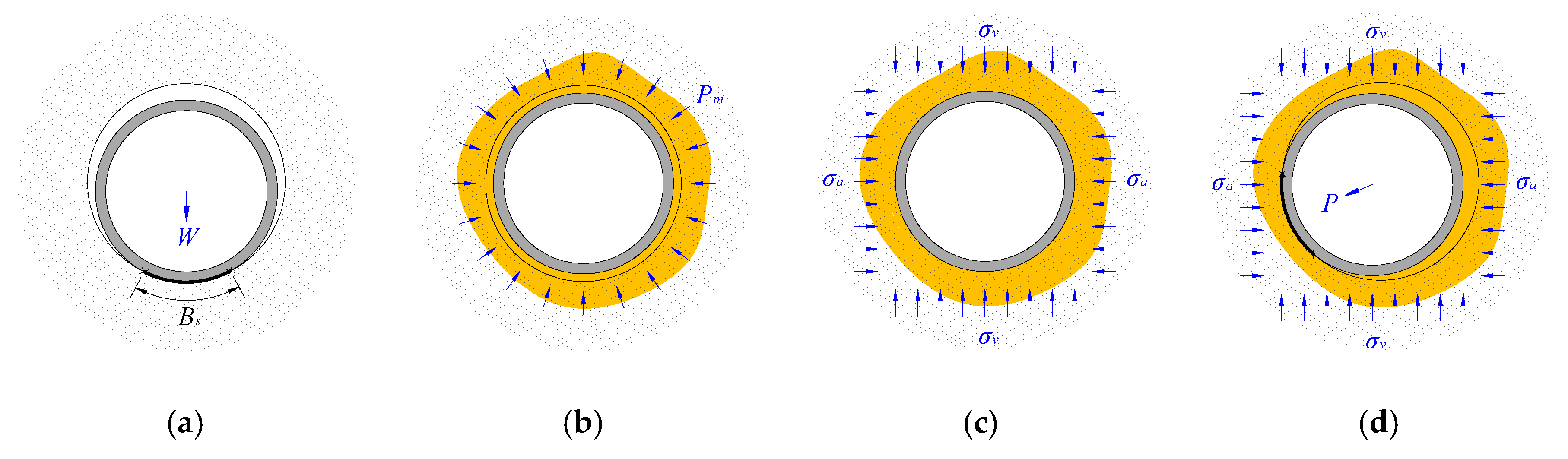
Some hypotheses have been made to establish the prediction models, by which one or some of the items listed above should be considered. Typical hypotheses are:

Hypothesis 1.

The excavated tunnel is self-stable, the pipeline simply slides along the bottom of the tunnel due to its own weight (see Figure 2a) [9,10,14].

Hypothesis 2.

The angular space due to overcut is completely filled with lubricant slurry, and the excavated tunnel is stable under the slurry pressure (see Figure 2b) [22,25].

Hypothesis 3.

The excavated tunnel is unstable, the surrounding soil collapses and is in full contact with the whole area of the jacking pipes (see Figure 2c) [5,6,9,21,26].

Hypothesis 4.

The excavated tunnel is stable under the pressure of slurry, and part of the pipe comes in contact with the surrounding soil (see in Figure 2d) [3].

According to Hypothesis 1, there are two kinds of prediction models, in which the item of f_w has to be taken into consideration. The first one assumes that the friction resistance is only due to the weight of pipe [9,21]. It is given as

$$f={\mu }_{s}W$$

(6)

$${\mu }_s=\tan (\phi /2)$$

(7)

The second one also takes the pipe-soil cohesion resistance (item of f_sc) into account [10,14,21], which is given by

$$f={\mu }_{s}W+c_s{B}_s$$

(8)

where the pipe-soil contact width B_s is calculated by Hertzian contact model, as [10,14,21]

$$B_s=1.6{(P{k}_d{C}_e)}^{1/2}$$

(9)

$$k_d=\frac{D_c{D}_p}{D_c-D_p}\begin{array}{cc},& \end{array}{C}_e=\frac{1-v_p^2}{E_p}+\frac{1-v_s^2}{E_s}$$

(10)

where D_c and D_p are the internal diameter of cavity and external diameter of pipe, respectively, m; ν_p and ν_s are the Poisson’s ratio for pipe and soil material, respectively; E_p and E_s are the elasticity modulus of the pipe and soil, respectively, kPa; and P is the effective external force acting on the center of the pipe, kN/m, usually it is considered as equal to the weight of pipe per unit length W.

According to Hypothesis 2, the friction resistance is related only to the properties of lubricant slurry, and the only model found was one that takes both the items of f_m and f_mc into account [22,25].

$$f={\mu }_{m}N+c_m{B}_m$$

(11)

$$N=\pi D_p{P}_m$$

(12)

$$B_m=\pi D_p$$

(13)

where P_m is the mud slurry pressure.

It is noted that most of the studies completed to date have focused exclusively on the prediction models established by Hypothesis 3. This may be attributed to the assumption of full contact of the pipe and soil that leads to a large prediction value of friction resistance, or in other words, Hypothesis 3 is conservative. Because of that, this kind of model is widely accepted by authorities and standards from all over the world, such as Japan Sewage Association (JSA) [22], UK Pipe Jacking Association (PJA) [27], Chinese Trenchless Technology Association (CTTA) [28], and Germany Standard (AVT A-161) [29]. This kind of model can be summarized and divided into the following four categories.

$$f={\mu }_{s}N$$

(14)

$$f={\mu }_{s}N+{\mu }_{s}W$$

(15)

$$f={\mu }_{s}N+{\mu }_{s}W+c_s{B}_s$$

(16)

$$f=\beta {\mu }_{s}N+{\mu }_{s}W+c_s{B}_s$$

(17)

The fourth kind of model (Equation (17)) introduces an empirical constant β (smaller than 1) on the basis of the third model (Equation (16)) to reflect the effect of lubrication.

For the models summarized above, the item of f_s (=μ_sN) has to be taken into consideration. Thus, the key problem for this kind of model is exactly focused on the calculation of soil pressure N. CTTA suggests N to be calculated by Rankine’s formula, which gives that [28]

$$N=2(1+K)D_p{\sigma }_v$$

(18)

$${\sigma }_v=\gamma h$$

(19)

$$K={\tan }^2(\pi /4-\varphi /2)$$

(20)

where σ_v is the vertical soil stress; K is the coefficient of soil pressure above the pipe; γ is the unit weight of soil; h is the overburden depth of the pipeline; and φ is the internal friction angle of soil.

However, JSA suggests using Terzaghi’s silo model, the expression of N is then expressed as [22]

$$N=\pi D_p{\sigma }_v$$

(21)

$${\sigma }_v=\frac{b\gamma -2c_s}{2K\tan (\delta )}\left(1-e^{-2K\tan (\delta )h/b}\right)$$

(22)

where c_s is the cohesion of soil; δ is the friction angle between the pipe and soil; b is the influencing silo width of soil above the pipe, and the other symbols have the same meanings as before.

Although a lot of prediction equations of friction resistance have been proposed and even some of them have been applied to engineering practice, it is obvious that their hypotheses are quite different, and even for the same hypothesis, models and parameters can be different too. Thus, it is bound to make the prediction friction resistances vary greatly. Furthermore, apart from Equations (11) and (17), the other models completely ignore the effect of lubrication, which is very important to slurry pipe jacking.

In the design philosophy of slurry pipe jacking, the angular space due to overcut is expected to be completely filled with lubricant slurry, to reduce the friction resistance with maximum efficiency, creating a ‘filter cake’ layer around the cavity and is then pressurized to the support pressure required for the soil (see Figure 2b) [3,10]. In this case, the friction resistance should be only related to the slurry pressure and the friction coefficient between slurry and the pipe. From this point of view, the expression Equation (11) seems a convincing explanation here.

However, the more general case is that the excavated tunnel is stable under pressure of slurry and part of the pipe inevitably comes in contact with the soil (see Figure 2d) [3]. The reasons for the occurrence of pipe-soil contact can be complex, such as insufficient design and control of grouting amount of slurry, the pipeline deviates from the intended line and level, irregular deformation of the surrounding soil, and interpenetration between the soil and slurry. Thereby, the state of contact can change from ‘pipe-slurry’ into ‘pipe-soil-slurry’ (Figure 2b,d). In such a case, a simple form of Equation (17) seems more suitable to reflect the effect of lubricant slurry. However, it is logical that the greater the contact width between the pipe and the soil, the smaller the effect of lubrication will be, and, therefore, the greater the friction resistance will be. Thus, the value of β should be highly affected by the pipe-soil contact width. For different soils, grouting amount of slurry and design parameters (such as buried depth and overcut) is bound to lead to completely different contact widths of pipe-soil. Thus, β should be in a large range, and it would be rather difficult to pick out a value to use in application.

In fact, a successful prediction model of friction resistance should not only consider the effect of lubrication but also needs to be able to reflect the effect of pipe-soil-slurry interaction. It is based on this understanding that the following model comes into being.

3. Calculation of Friction Resistance for Slurry Pipe Jacking

The general contact state of pipe-soil-slurry due to the interaction of the pipe, surrounding soil, and lubricant slurry is shown in Figure 3. In the picture, the position of pipe-soil contact is arbitrary, with a contact width of B_s and the corresponding contact angle of 2ε.

From Figure 3, it is obvious that to calculate friction resistance f, both of the items of f_s and f_m have to be taken into account, which can be expressed as

$$f=\mu N=f_s+f_m={\mu }_s{N}_s+{\mu }_m{N}_m$$

(23)

where μ is an effective friction coefficient introduced to reflect the effect of lubrication and the influence of pipe-soil contact width. It is generally accepted that μ_s = tan(φ/2) for the coefficient of kinematic friction between soil and the pipe [21,22]; μ_m for the coefficient of kinematic friction between mud slurry and the pipe can be taken as 0.01, according to the test result reported by Guo [30]. N_s and N_m are the total normal force of pipe-soil and pipe-slurry in contact, respectively.

To calculate N_s and N_m precisely, the location of pipe-soil contact and the magnitude of contact angle (or contact width) and the contact force have to be determined. For various reasons leading to the occurrence of pipe-soil contact, it seems impossible to calculate these quantities in a target section of the pipeline. However, if taking the whole pipeline into consideration, and assuming that the pipe-soil contact can occur at any position of a section of the pipeline with a same probability and the contact force is approximately equal to the soil pressure in the contact area, this problem can be greatly simplified. In this case, we have the following equations:

$$P=N_s=\frac{B_s}{C}N=\frac{\epsilon }{\pi }N$$

(24)

$$N_m=\frac{B_m}{C}N$$

(25)

where C (=πD_p) is the external circumference of pipe and ε is the semi-angle of contact (Figure 3).

By substituting Equations (24) and (25) in Equation (23), after some algebra, giving that

$$\begin{array}{l}\mu ={\mu }_s{\lambda }_s+{\mu }_m{\lambda }_m\\ {\lambda }_s=\frac{B_s}{C}=\frac{\epsilon }{\pi }\begin{array}{cc},& {\lambda }_m=\frac{B_m}{C}\end{array}\end{array}$$

(26)

$$B_m=C-\frac{B_s}{1+e}$$

(27)

where e is the void ratio of soil.

By substituting Equation (27) in Equation (26), the expression of μ can be further rewritten as

$$\mu ={\mu }_s\frac{\epsilon }{\pi }+{\mu }_m\left(1-\frac{\epsilon }{\pi (1+e)}\right)$$

(28)

According to Equation (28), the calculation of ε is essential to calculate μ. Hertzian model provides a simple way for the calculation of the width of contact (or contact angle) as we have mentioned before (see Equations (8) and (10)); however, the Hertzian contact problem is approached only when the applied force is small, or the large radial clearance is large, and the limited angle of contact is smaller than about 30° [31]. Due to the technical limitations, most of the pipe jacking projects encounter clay or sandy soils and with a small overcut, it is therefore important that the applicability of the Hertzian contact model should be extremely limited here. Actually, the Hertzian contact model is just a special case of the Persson’s contact model with a small contact width (or angle) [31]. If a large contact angle (larger than 30°) occurs, the more general contact model proposed by Persson should be taken as the first choice. The following singular integro-differential governing equation of contact angle is derived by Persson, as [31,32]

$$B=4(1-\beta )-2(1-\alpha ){\displaystyle \underset{-\xi }{\overset{+\xi }{\int }}q(t)\frac{dt}{1+t^2}}-\frac{\pi }{2}(1+\alpha )\frac{E_p\Delta R}{(1-v_p^2)P}$$

(29)

or

$$\frac{\pi (1+\alpha )E_p\Delta R}{(1-v_p^2)P}=4(1-\beta )-2(1-\alpha ){\displaystyle \underset{-\xi }{\overset{+\xi }{\int }}q(t)\frac{dt}{1+t^2}}-B$$

(30)

The involved auxiliary variables are defined as [31]

$$\begin{array}{l}\Delta R=\frac{D_c-D_p}{2}\begin{array}{cc},& \xi =\tan \left(\frac{\epsilon }{2}\right)\begin{array}{cc},& \end{array}\end{array}\\ \alpha =\frac{1-\eta }{1+\eta }\begin{array}{cc},& \beta =\frac{\lambda }{2(1+\eta )}\end{array},\\ \eta =\frac{E_p}{E_s}\frac{1-v_s^2}{1-v_p^2}\begin{array}{cc},& \lambda =\end{array}\frac{1-2v_p}{1-v_p}-\eta \frac{1-2v_s}{1-v_s}\end{array}$$

(31)

After some approximate treatments, the key terms of Equation (30) have been solved by Michele [32], as follows:

$${\displaystyle \underset{-\xi }{\overset{+\xi }{\int }}q(t)\frac{dt}{1+t^2}}=\frac{1}{2\pi }\frac{I_b}{{\xi }^2({\xi }^2+1)}+\frac{{\xi }^2}{{\xi }^2+1}$$

(32)

$$I_b=\pi \log ({\xi }^2+1)$$

(33)

$$B=\frac{2{\xi }^4+2{\xi }^2-1}{{\xi }^2({\xi }^2+1)}$$

(34)

By substituting these equations into Equation (29), Michele obtained an approximate form of general contact angle relation.

$$\frac{\pi (\alpha +1)E_p\Delta R}{(1-v_p^2)P}=\frac{(\alpha -1)[\ln ({\xi }^2+1)+2{\xi }^4]+2}{({\xi }^2+1){\xi }^2}-4\beta$$

(35)

As compared with Equation (9), Equation (35) is a far more complex nonlinear equation. It can be further simplified with respect to that the elastic modulus of soil E_s is generally much smaller than that of pipe E_p (the difference between the two can be three orders of magnitude). Thus, from Equation (30), the magnitude of auxiliary variable η should be very large, and, therefore, the following approximate relations can be obtained:

$$\begin{array}{l}\frac{\pi (\alpha +1)E_p}{(1-v_p^2)}\approx \frac{2\pi E_s}{(1-v_s^2)},\\ \alpha \approx -1,\\ \beta \approx \frac{1-2v_s}{2(1-v_s)}\end{array}$$

(36)

Using Equation (36), Equation (35) can be then simplified as

$$\frac{\pi E_s\Delta R}{(1-v_s^2)P}+\frac{1-2v_s}{1-v_s}=\frac{1-[\ln ({\xi }^2+1)+2{\xi }^4]}{({\xi }^2+1){\xi }^2}$$

(37)

From Equation (37), it is essential to calculate P, which requires one to calculate the total normal force N. It can be gained by integrating the normal stress σ_n on an element of the pipe surface and is determined on the basis of vertical and horizontal soil stresses.

$${\sigma }_n={\sigma }_v\sin \theta +{\sigma }_a\cos \theta$$

(38)

$$N=4{\displaystyle {\int }_0^{\pi /2}{\sigma }_n\frac{D_p}{2}}d\theta$$

(39)

where θ is defined as the angle between the corresponding radius line and the horizontal line at each point of the pipe (Figure 4).

By substituting Equation (38) in Equation (39), it is easy to obtain the equation of N, which has the same form as Equation (18).

To calculate Equation (18), the vertical soil stress σ_v has to be first determined. It is noted that at the present time, by far the most commonly used model for soil pressure calculation is Terzaghi’s silo model (Equation (22)) [5,6,9,19,21,26]. According to Equation (22), the calculation of the vertical soil stress requires some physical parameters that may be determined with some accuracy, such as the height of cover h, the cohesion c_s, and the unit weight of soil γ, but also some empirical parameters, such as b, δ, and K. The definition of these empirical parameters varies from one author to another. Here, typical approaches of Terzaghi, Germany Standard ATV-A 161 E-90 [29], Chinese Standard GB 50332-2002 [33], UK Standard BS EN 1594-09 [34], US Standard ASTM F 1962-11 [35], UK PJA [27], Japan JMTA [36], and Japan JSA [22] would be discussed and compared.

For the calculation of silo width b, three kinds of boundary planes of wedge failure assumed by different authors and the corresponding equations are clearly illustrated in Figure 5. The width of the boundary plane is related to the ‘vault’ effect of soil. Generally, a smaller b means a lower ‘vault’ effect of soil, leading to a larger vertical soil stress.

For the determination of δ, most of the guidelines, such as PJA, JSA, JMTA, BS EN 1594-90, and GB 50332-2002 assume shear planes as perfectly rough and take an angle of friction in the shear planes δ equal to the soil internal friction angle φ. However, ATV-A 161 E-90 and ASTM F 1962-11 make a more cautious assumption and only takes into account half the internal friction angle φ/2.

For the lateral pressure coefficient K above the tunnel, Terzaghi assumes K coefficient is equal to 1, which corresponds to the range of values encountered in clayey soils. PJA, ASTM F 1962-11, and GB 50332-2002 suggest K = K_a (calculated by Rankine’s formula of active soil pressure coefficient), while BS EN 1594 and ATV-A 161 assume K = K₀ (calculated by Rankine’s formula of soil pressure coefficient at rest). Moreover, according to ATV-A 161, this K coefficient is equal to 0.5, which corresponds to an internal soil friction angle of 30°, a typical value for sandy soils.

Parameters of b, δ, and K chosen by the different authors have been summarized in

Table 1. Definition of the empirical parameters in Terzaghi’s silo model by different authors [37].

Parameters	b	δ	K	c
Terzaghi (Japan)	Dp(1 + 2tan α)	φ	1	c
JMTA (Japan)	(Dp + 0.08)tan β	φ	1	c
JSA (Japan)	(Dp + 0.1)tan β	φ	1	c
PJA (UK)	Dptan β	φ	Ka = tan2 α	c
BS EN 1594 (UK)	Dp(1 + 2tan α)	φ	K0= 1 − sin φ	c
AVT A-161 (Germany)	1.732Dp	φ/2	K0 = 0.5	None
ASTM F 1962-11 (US)	1.5Dp	φ/2	Ka = tan2 α	None
GB 50332-2002 (China)	Dp(1 + tan α)	φ	Ka = tan2 α	None

Note: α = π/4 − φ/2; β = π/4 + α/2.

.

It is noted that none of the approaches use the same parameters. Consequently, the vertical soil stress calculated by these approaches would be quite different. Thus, it is not convincing to pick out an approach to use without checking the field data. This work will be carried out in the next section.

Thus far, all the equations needed to calculate friction resistance have been determined. If the parameters needed for the prediction equations are quantified, by using Equations (18) and (22) the total normal force N can be determined, then together with Equations (23), (24), (27), (31), and (37), the contact angle 2ε, the effective friction coefficient μ, and the friction force f now can be uniquely identified. The flow chart is shown in Figure 6.

Apparently, the effective friction coefficient here is not just related to the interfriction angle of soil φ but also the state of pipe-soil contact and the effect of lubrication.

4. The Verification of the Effectiveness of the Proposed New Approach

4.1. Comparison between the Predicted Friction Resistances and the Field Data

Before comparison analysis, the existing prediction equations were numbered from M 1 to M 13 (

Table 2. The numbering of the existing friction resistance prediction equations.

Number of Models	Equations	Approaches
M 1	Equations (6) and (7)
M 2	Equations (7)–(10)
M 3	Equations (7), (11) and (12)
M 4	Equations (7), (15), (18) and (19)	CTTA (China)
M 5	Equations (7), (16), (21) and (22)	JSA 1 (Japan)
M 6	Equations (7), (17), (21) and (22)	JSA 2 (Japan)
M 7	Equations (7), (14), (18) and (22)	JMTA (Japan)
M 8	Equations (7), (14), (18) and (22)	Terzaghi (Japan)
M 9	Equations (7), (14), (18) and (22)	PJA (UK)
M 10	Equations (7), (14), (18) and (22)	BS EN 1594-09 (UK)
M 11	Equations (7), (14), (18) and (22)	ATV A 161 E-90 (Germany)
M 12	Equations (7), (14), (18) and (22)	ASTM F 1962-11 (US)
M 13	Equations (7), (14), (18) and (22)	GB 50332-2002 (China)

). For M 7~M 13, the Equations (7), (14), (18), and (22) should be used and the parameters (b, δ, and K) of Terzaghi’s silo model (Equation (22)) in the calculation of earth pressure should be determined by their approaches that are shown in Table 1.

As has been mentioned before, the new approach of this paper introduces an effective friction coefficient μ (Equation (28)) to replace the original pipe-soil friction coefficient μ_s (Equation (7)). The calculation of μ (Equation (28)) should follow the flow chart shown in Figure 2. Equations (18) and (22) are also used to calculate the normal force N and vertical earth pressure σ_v, respectively. The new prediction equations were numbered from M 7 * to M 13 * (

Table 3. The numbering of the new friction resistance prediction equations.

Number of Models	Equations	Approaches
M 7 *	Equations (14), (18), (22) and (28)	JMTA (Japan)
M 8 *	Equations (14), (18), (22) and (28)	Terzaghi (Japan)
M 9 *	Equations (14), (18), (22) and (28)	PJA (UK)
M 10 *	Equations (14), (18), (22) and (28)	BS EN 1594-09 (UK)
M 11 *	Equations (14), (18), (22) and (28)	ATV A 161 E-90 (Germany)
M 12 *	Equations (14), (18), (22) and (28)	ASTM F 1962-11 (US)
M 13 *	Equations (14), (18), (22) and (28)	GB 50332-2002 (China)

The superscript “*” is used to distinguish from the number of models in Table 2.

).

Some parameters required by the predicted equations (such as μ_s, P_m, and W) might not be given in the literature. In principle, during the calculation, the parameters given in the field case should be used, and the missing parameters can be evaluated by the following rules:

• The pipe-soil friction coefficient μ_s is uniformly calculated by μ_s = tan (φ/2).
• The slurry pressure P_m is usually set as equal to the vertical soil stress σ_v plus 30 kPa [28], so P_m = σ_v + 30 kPa is adopted.
• The weight of pipe W is evaluated by W = γ_pS, where γ_p = 24 kN/m³ is for reinforced concrete [38], S is the area of pipe cross section.
• When the overcut ΔR (usually between 0~50 mm) is missed, ΔR = 10 mm is taken.
• The cohesion of pipe-slurry c_m is usually less than 0.1 kPa [39], c_m = 0.1 kPa is used.
• The average values of soil parameters (such as γ_s, c_s, φ, and e) can be obtained from the Geological Engineering Handbook.

Parameters in each of the four cases were finally determined, which are given in

Table 4. Parameters that are needed to calculate the prediction equations in each case.

Cases		C 1 (H City)	C 2 (Shanghai)	C 3 (F City)	C 4 (Neuilly)
Geotechnical Description		Organic Silt	Silty Clay	Fine Sand	Sand and Gravels
Parameters	h (m)	8.15	8.5	2.72	5
	Dp (m)	0.96	4.06	1.2	0.66
	ΔR (mm)	10	20	10	0
	γ (kN/m3)	18	19.5	20.5	21
	cs (kPa)	10	30	0	0
	φ (°)	10	25	30	40
	Es (MPa)	12	25	30	35
	vs	0.35	0.3	0.25	0.2
	e	2	1.5	1	0.4
	cm (kPa)	0.1	0.1	0.1	0.1
	β	0.6	0.5	0.85	0.5
	W (kN/m)	5.5	90.2	8.5	2.2
	μm	0.01	0.01	0.01	0.01
	Pm (kPa)	89.97	110.54	62.28	45.94

[2,9,22]. These cases encountered some representative soils, such as silt, clay, sand, and gravels. Furthermore, they have different overburden depths of 2.72~8.5 m, overcut of 0~20 mm, and pipe diameters of 0.66~4.06 m. All of these characteristics provide good foundations for identifying the capability of the prediction models.

In

Table 5. Comparison of friction resistances calculated by the existing models and the measured data.

Cases		C 1		C 2		C 3		C 4
			Ratio		Ratio		Ratio		Ratio
fmea.(kN/m)		1.5		36.16		3.78		9.75
fcal.(kN/m)	M 1	0.48	32%	20.00	55%	2.28	60%	0.80	8%
	M 2	2.68	179%	76.10	210%	2.28	60%	0.80	8%
	M 3	3.02	201%	15.37	43%	2.72	72%	1.16	12%
	M 4	42.47	2832%	439.47	1215%	50.09	1325%	62.22	638%
	M 5	39.72	2648%	575.39	1591%	32.65	864%	12.06	124%
	M 6	38.36	2557%	489.02	1352%	20.50	542%	6.43	66%
	M 7	11.14	743%	218.77	605%	38.35	1014%	13.96	143%
	M 8	14.28	952%	267.04	738%	41.52	1098%	15.32	157%
	M 9	9.42	628%	198.74	550%	37.56	994%	28.88	296%
	M 10	16.68	1112%	247.43	684%	40.31	1066%	26.36	270%
	M 11	30.06	2004%	392.61	1086%	45.37	1200%	37.86	388%
	M 12	30.24	2016%	370.94	1026%	41.90	1108%	42.29	434%
	M 13	24.99	1666%	332.53	920%	36.72	972%	27.63	283%

Note: f_mea. is the measured friction resistance; f_cal. is the calculated friction resistance.

, for each of the drives, measured frictional force values are presented and compared to values calculated by the approaches of the existing models. One can see that, for most cases, the prediction results of the models (M 1 and M 2) established based on Hypothesis 1 are generally too small. This is because it is correct only when the overcut is stable and the pipeline slides on its base inside the annular gap remaining open. The same problem is encountered in M3 (established based on Hypothesis 2), which is probably more due to ignoring the occurrence of pipe-soil contact decreasing the magnitude of the effective friction coefficient. Obviously, for slurry pipe jacking, the prediction friction based on these two assumptions may be insufficient and unsafe.

The calculated results of M4 are much larger than the measured data, which presumably result from ignoring the ‘vault effect’ of soil, so that the soil pressure has been overestimated. Apart from M4, the other models established based on Hypothesis 3 (M5~13) have shown some applicability in case 4, in which the overcut of C4 is equal to zero, which is exactly in line with the assumption of the full contact of pipe-soil of Hypothesis 3. Except for C4, the prediction results of other cases are much larger, and the amplitude may be up to 30 times the measured data. Therefore, for slurry pipe jacking, Hypothesis 3 is generally over-conservative. Although it can ensure the structural safety of the design, it may also cause a much higher construction cost.

From what we have analyzed above, the existing models have good prediction results only when the field case is consistent with the basic hypothesis of each model. However, it is also these hypotheses that determine their limited applicability.

Table 6. Comparison of the friction resistances calculated by the new approach and the measured data.

Cases		C 1		C 2		C 3		C 4
			Ratio		Ratio		Ratio		Ratio
fmea.(kN/m)		1.5		36.16		3.78		9.75
fcal.(kN/m)	M 7 *	2.44	163%	43.37	120%	3.55	94%	5.19	53%
	M 8 *	3.46	231%	58.53	162%	4.02	106%	5.69	58%
	M 9 *	1.93	129%	41.19	114%	3.43	91%	10.74	110%
	M 10 *	4.30	287%	56.99	158%	3.84	101%	9.80	101%
	M 11 *	2.09	140%	48.22	133%	4.62	122%	14.08	144%
	M 12 *	1.26	84%	36.51	101%	4.08	108%	15.72	161%
	M 13 *	1.89	126%	35.02	97%	3.31	88%	10.27	105%

The superscript “*” is used to distinguish from the number of models in Table 2.

presents the friction resistances calculated by the approach of this paper, by using the parameters of Terzaghi silo model chosen from different authors (Table 1). Better agreements with the field data in each of these cases were obtained, which indicate that compared with the existing prediction models, the approach of this paper that considers the effect of lubrication and interaction of pipe-soil-slurry not only has higher accuracy but is also more flexible and has wider applicability.

Moreover, the approaches of PJA (M9), ATV A 161 E-90 (M11), ASTM F 1962-11 (M12), and GB 50332-2002 (M13) provide higher prediction accuracy than the other ones (Table 6). However, it is noted that ATV A 161 E-90, ASTM F 1962-11, and GB 50332-2002 suggest the effect of soil cohesion c should be neglected (Table 1), but it is because the cohesion of soil has been considered in the calculation that the good prediction results can be obtained, as shown in Table 6. From this point of view, UK PJA (consider the cohesion of soil) provides the best choice of parameters of Terzaghi’ silo model in the calculation of earth pressure. Therefore, the UK PJA approach is supposed to be used in the next analyses.

4.2. Comparison between the Predicted Friction Resistances and the Numerical Simulation Result

Some excellent work of numerical simulation has been conducted for the estimation of the jacking force (or friction resistance) of pipe jacking. For example, Ji et al. [5,40] and Barla and Camusso [41] presented a novel discrete 2D numerical model to evaluate the normal force acting on the pipe. Then, the friction resistance is determined by multiplying the interface friction coefficient by the normal force. Three different drives in a pipe jacking projects were analyzed, where the calculated pattern of jacking force was compared with the measured data, which demonstrated the effectiveness of the proposed approach. Yen and Shou [25] used a model coupling finite element method and a displacement control method to estimate the required jacking force in pipe jacking. The displacement control option in the numerical analysis software ABAQUS (Abaqus Inc., (Palo Alto, CA, USA) 2012) was used to designate the displacement at the end cross section of the pipe in the launch shaft. Accounting for the contact property and the contact range between the pipes and the soil during the jacking process, the stresses exerted on the pipes were used to back-calculate the jacking forces [25].

The numerical simulation strategy of Yen and Shou [25] is quite consistent with the analytical approach of this paper. Therefore, the numerical simulation approach of Yen and Shou will be described in the next section and its estimated result of friction resistance will be discussed and compared with that calculated by the analytical approach of this paper.

One of the analyses focused on a case of slurry pipe jacking in the Taichung Science Park, the basic parameters of this case were summarized in

Table 7. The details of the slurry pipe jacking in Taichung Science Park.

Geology	h (m)	Dp (m)	ΔR (mm)	γ (kN/m3)	c (kPa)	φ (°)	Es (MPa)	vs	e
Gravel	13.0	2.85	10	21	15	37	33	0.20	1

. In the numerical simulation, the lateral boundaries were fixed by roller, and hinges were used to constrain the bottom boundary. The three dimensional hexahedron element (C3D8R) with eight nodes was used in the simulation. To verify the jacking force obtained from the displacement control simulation, overcut and lubrication were included in the model by setting the contact range (1/3, 1/2, and 1 pipe-soil contact) and the frictional coefficient (Figure 7a–c). The results suggested the 1/3 contact case can estimate the jacking force with a better accuracy towards the middle and the final stage of the pipe jacking process (Figure 8).

In Figure 8, the slope of the linear regression for the scattered points represents frictional resistance, and the intercept represents face resistance. For the calculated result of this paper, the measured face resistance is used, and the frictional resistance (f_cal. = 57.7 kN/m) is calculated by the new approach (Section 3) using parameters of UK PJA in Terzaghi’s silo model (Table 1). For the result of numerical simulation, the decrease of jacking force in the initial stage of drives (before 62.5 m) is explained by authors that the weight of the pipe jacking machine (the material of which is steel, featuring a larger unit weight) directly pressing on the soil, causing a larger face resistance. After the drives of 62.5 m, the influence exerted by the machine weight decreased gradually and the increase of jacking force is caused by the accumulation of friction resistance [25]. In other words, the slope of regression from drives of 62.5 to 100 m represents the friction resistance estimated by numerical simulation (f_num. = 64.4 kN/m).

It is obvious that both the predicted friction resistances of the analytical equations (f_cal. = 57.7 kN/m) and the numerical simulation (f_num. = 64.4 kN/m) are acceptable as compared to the measured data (f_mea. = 41.5 kN/m). However, better accuracy (especially towards the first 80 m of drives) is obtained by the approach of this paper.

The predicted accuracy of friction resistance by the numerical simulation approach is highly affected by the setting of pipe-soil contact angle. The pipe-soil contact angle of 71 degrees is that calculated by the analytical equations for this field case. Thus, it seems that the pipe-soil contact angle of 120 degrees (1/3 contact) in the simulation is set too large, resulting in the calculated result slightly larger than the measured data. From this point of view, the numerical simulation approach can accurately predict the friction resistance, but the contact angle of pipe-soil in the simulation needs to be set reasonably to obtain good prediction results. Conversely, in the approach of this paper, the pipe-soil contact angle is theoretically calculated with respect to soil property, overcut, pipe diameter, etc., while human factors or empirical factors can be eliminated as far as possible.

5. Influence of Design Factors on Lubrication Efficiency and Friction Resistance

For a better design of slurry pipe jacking in the future, it is meaningful to study the influence of design parameters (such as buried depth h, pipe diameter D_p, and the overcut ΔR) on lubrication efficiency and friction resistance. To achieve this objective, a set of reference parameters is used, and then, by changing a target parameter according to the design rules, the effect of that parameter on friction resistance and lubrication efficiency can be obtained. The designed cases were shown in

Table 8. The reference parameters and cases designed to study the influence of factors on friction resistance.

Reference Parameters	h = 10 m, Dp = 2 m, ΔR = 20 mm, γ = 20 kN/m3, cs = 15 kPa, φ = 25°, Es = 25 Mpa, vs = 0.25, e = 1, μm = 0.01
Designed cases	h (m)	5→8→10→15→20→25→30
	Dp (m)	1→1.5→2→2.5→3→3.5→4
	ΔR (m)	0→5→10→20→30→40→50

.

5.1. Influence of Design Factors on Friction Resistance

The influences of design factors (h, D_p, and ΔR) on the critical quantities of effective friction coefficient μ, normal force acting on the pipe N, and friction resistance f are respectively shown in Figure 9a–c, Figure 9d–f, Figure 9g–i.

It is evident that increasing buried depth and pipe diameter led to a double action for the increasing of friction resistance. Firstly, this increase then increased the possibility of contact between the pipe and soil, and, therefore, increase the effective friction coefficient μ on the interface. Secondly, the increasing of buried depth increases the vertical soil stress, while the increasing of pipe diameter increases the contact area, both effects of them increase normal force N acting on the pipes. The main difference between the two is that buried depth causes both of the effective friction coefficient and normal force to slightly increase and then gradually stabilize, while they approximately linearly increase with pipe diameter. Especially for the normal force induced by pipe diameter, which is strongly increased from 29.83 to 991.34 kN, this leads to a notable increase of friction resistance from 0.34 to 48.16 kN/m. Thus, the additional friction is strongly affected by the pipe diameter but appears not to be greatly affected by the buried depth.

Different from the buried depth and pipe diameter, the overcut with small values has no effect on the normal force (Figure 9h). However, it has a strongly negative effect on the effective friction coefficient on the interface (Figure 9g). In fact, it does determine the volume of injected lubricant slurry, which has a significant influence on the occurrence of the pipe-soil contact, and, therefore, determine the magnitude of the effective friction coefficient. Thus, it has a strongly negative effect on the friction resistance.

5.2. Influence of Design Factors on Lubrication Efficiency

Except for friction resistance, engineers are also concerned about the lubrication efficiency [9,42,43]. According to Equation (27), the magnitude of μ is between the pipe-slurry friction coefficient μ_m and the pipe-soil friction coefficient μ_s. If there is no contact between the pipe and the soil, the angular space due to overcut is completely filled with lubricant slurry, the effective friction coefficient is equal to μ_m; and if the soil is in full contact with the external surface of the pipe, the effective friction coefficient mainly depends on the pipe-soil nature and approximately equals to μ_s. Thus, the lubrication efficiency can be defined as

$$\chi =\left(1-\frac{\mu -{\mu }_m}{{\mu }_s}\right)\times 100\%$$

(40)

By substituting Equation (28) in Equation (31), and considering that μ_m is far smaller than μ_s, the χ can approximately be expressed by Equation (41).

$$\chi =\left(1-\frac{\epsilon }{\pi }\right)\times 100\%$$

(41)

If pipe-soil contact angle ε = 0, χ = 100% for maximum lubrication efficiency, and if ε = π, χ = 0% for minimum lubrication efficiency. It is noted that χ = 0% is not going to happen. According to the Passon model (Equation (37)), the result calculated by the left terms of Equation (37) should be not less than zero, while the right term of Equation (37) is a monotonically decreasing function of pipe-soil contact angle. In other words, when the right term of Equation (37) is equal to zero, the pipe-soil contact angle reaches its maximum value, which is solved by ε = ε_max = 72° = 0.4π, corresponding to the minimum lubrication efficiency of 60% (i.e., χ is theoretically between 60% and 100% on the basis of Passon contact model). Although it is not theoretically correct as compared to that counted by Pellet and Kastner as between 45% and 90% [9] and tested by Zhou as between 47.8% and 78.6% [5], it seems practical to estimate the efficiency of lubrication by the approach of this paper.

The pipe-soil contact angle and the corresponding lubrication efficiency calculated by Equation (41) has been shown in Figure 10a–c, Figure 10d–f, respectively. It is found that, as compared to the low effect of overburden depth, special attention should be paid to the effect of pipe diameter and the overcut.

Figure 10f shows that the lubrication efficiency strongly increases from 64% to 91%, while the overcut increases only from 0 to 15 mm, and after that, the effect of overcut is significantly reduced. This observation confirms the importance of overcut, which has to be sufficiently wide so that the decrease of tunnel diameter induced by the elastic ground unloading does not lead to the closure of the annular space. Moreover, Figure 10e shows that the increasing of pipe diameter from 1 to 4 m causes obvious efficiency losses of lubrication from 99% to 82%. Thus, one can conclude that the larger the pipe diameter, the lager the overcut is needed.

The buried depth h is determined by the intended line and level of the tunnel, which is often limited by geological conditions and distributions of the existing buildings and structures, while the pipe diameter D_p highly depends on the practical use or traffic requirements. It seems that there are not many options for the buried depth h and pipe diameter D_p in the design. From this point of view, both for lubrication efficiency and friction reaction, more attention should be paid to the design of overcut.

Parts of the conclusions analytically discussed above have been verified by authors from field observations [9,20], which in turn again confirm the feasibility of the approach of this paper.

6. Conclusions

Some typical prediction models of friction resistance have been presented and detailed comparisons and analyses have also been made. Then, a new approach considering both the effect of lubrication and the interaction of pipe-soil-slurry, by introducing an effective friction coefficient, has been established. Values of friction resistance calculated using them have been compared with values measured in four field cases and a numerical simulation case with various soils and design parameters. Better agreements are obtained, which indicate a more flexible and wider applicability of the approach in this paper as compared to the existing prediction models and numerical simulation approach. Explanations have also been sought for limited use of the existing models that may be attributed to their hypotheses not that suitable for slurry pipe jacking. The numerical simulation approach can accurately predict the friction resistance, but it is hard to determine the contact angle of pipe-soil reasonably with respect to various soils, overcut, and other conditions to obtain good prediction results.

Using the approach of this paper, for higher prediction accuracy, the cohesion of soil has to be taken into account in the calculation for drives in clayey soils. The Terzaghi’s silo model together with parameters determined by the approach of UK PJA is verified as the most well-considered to calculate earth pressure.

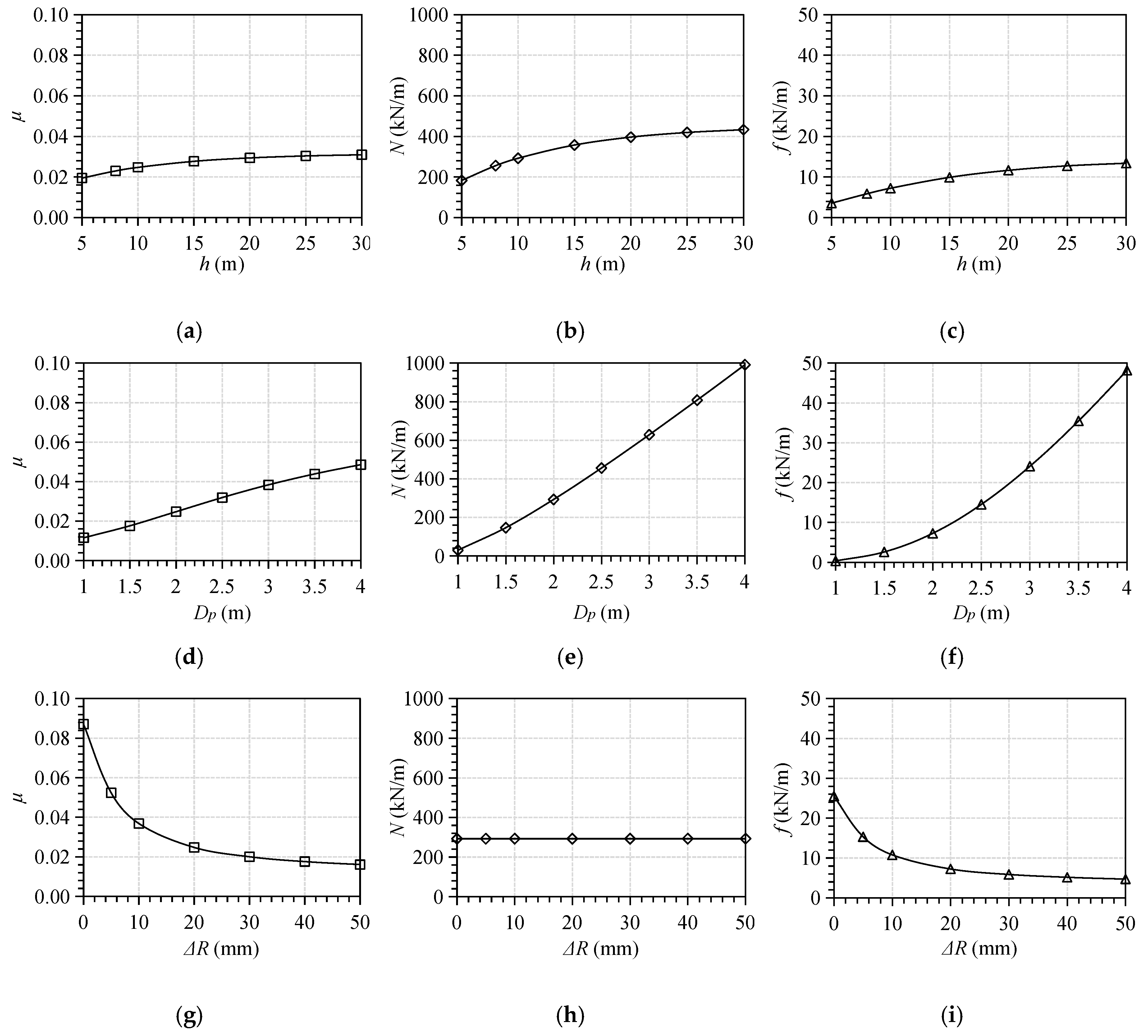
For better design in the future, the influences of design factors (buried depth, pipe diameter, and overcut) on friction resistance and lubrication efficiency have been analyzed too. The increase of pipe diameter has a strong influence on the increase of friction resistance; however, the friction amplitude appears not to be greatly affected by the buried depth. As the selection of pipe diameter and buried depth are limited by various objective conditions, special attention should be paid on the design of overcut. The overcut has to be sufficiently wide. When the overcut is small (for example smaller than 15 mm), the decrease of overcut strongly affects the decrease of lubrication efficiency, and, therefore, leads to a notable increase in friction resistance. Moreover, pipe diameter has an obvious influence on the effect of overcut on lubrication efficiency, the larger the pipe diameter the larger the overcut needed.

References

1. Ji, X.; Zhao, W.; Jia, P.; Qiao, L.; Barla, M.; Ni, P.; Wang, L. Pipe Jacking in Sandy Soil under a River in Shenyang, China. Indian Geotech. J. 2017, 47, 246–260. [Google Scholar] [CrossRef]
2. Wang, J.F.; Wang, K.; Zhang, T.; Wang, S. Key aspects of a DN4000 steel pipe jacking project in China: A case study of a water pipeline in the Shanghai Huangpu River. Tunn. Undergr. Space Technol. 2018, 72, 323–332. [Google Scholar] [CrossRef]
3. Khazaei, S.; Shimada, H.; Kawai, T.; Yotsumoto, J.; Matsui, K. Monitoring of over cutting area and lubrication distribution in a large slurry pipe jacking operation. Geotech. Geol. Eng. 2006, 24, 735–755. [Google Scholar] [CrossRef]
4. Ji, X.; Ni, P.; Barla, M.; Zhao, W.; Mei, G.X. Earth pressure on shield excavation face for pipe jacking considering arching effect. Tunn. Undergr. Space Technol. 2018, 72, 17–27. [Google Scholar] [CrossRef]
5. Ji, X.; Zhao, W.; Ni, P.; Barla, M.; Han, J.; Jia, P.; Chen, Y.; Zhang, C. A method to estimate the jacking force for pipe jacking in sandy soils. Tunn. Undergr. Space Technol. 2019, 90, 119–130. [Google Scholar] [CrossRef]
6. Ong, D.E.L.; Choo, C.S. Assessment of non-linear rock strength parameters for the estimation of pipe-jacking forces. Part 1. Direct shear testing and backanalysis. Eng. Geol. 2019, 244, 159–172. [Google Scholar] [CrossRef]
7. Ren, D.J.; Xu, Y.S.; Shen, J.S.; Zhou, A.; Arulrajah, A. Prediction of ground deformation during pipe-jacking considering multiple factors. Appl. Sci. 2018, 8, 1051. [Google Scholar] [CrossRef] [Green Version]
8. Zhang, Y.; Yan, Z.G.; Zhu, H.H. A full-scale experimental study on the performance of jacking prestressed concrete cylinder pipe with misalignment angle. In Proceedings of Geo. Shanghai 2018 International Conference: Multi-physics Processes in Soil Mechanics and Advances in Geotechnical Testing; Springer: Singapore, 2018; pp. 345–354. [Google Scholar]
9. Pellet-Beaucour, A.L.; Kastner, R. Experimental and analytical study of friction forces during microtunneling operations. Tunn. Undergr. Space Technol. 2002, 17, 83–97. [Google Scholar] [CrossRef]
10. Milligan, G.W.E.; Norris, P. Pipe-soil interaction during pipe jacking. Proc. Inst. Civ. Eng. Geotech. Eng. 1999, 137, 27–44. [Google Scholar] [CrossRef]
11. Shou, K.J.; Yen, J.; Liu, M. On the frictional property of lubricants and its impact on jacking force and soil-pipe interaction of pipe-jacking. Tunn. Undergr. Space Technol. 2010, 25, 469–477. [Google Scholar] [CrossRef]
12. Yang, X.; Liu, Y.; Yang, C. Research on the slurry for long-distance large-diameter pipe jacking in expansive soil. Adv. Civ. Eng. 2018, 2018, 9040471. [Google Scholar] [CrossRef]
13. Sterling, R.L. Developments and research directions in pipe jacking and microtunneling. Undergr. Space 2018, in press. [Google Scholar] [CrossRef]
14. Milligan, G.W.E.; Norris, P. Site-based research in pipe jacking-objectives, procedures and a case history. Tunn. Undergr. Space Technol. 1996, 11, 3–24. [Google Scholar] [CrossRef]
15. Cui, Q.L.; Xu, Y.S.; Shen, S.L.; Yin, Z.-Y.; Horpibulsuk, S. Field performance of concrete pipes during jacking in cemented sandy silt. Tunn. Undergr. Space Technol. 2015, 49, 336–344. [Google Scholar] [CrossRef]
16. Cheng, W.C.; Ni, J.C.; Arulrajah, A.; Huang, H.W. A simple approach for characterising tunnel bore conditions based upon pipe-jacking data. Tunn. Undergr. Space Technol. 2018, 71, 494–504. [Google Scholar] [CrossRef]
17. Cheng, W.C.; Ni, J.C.; Shen, S.L.; Huang, H.W. Investigation into factors affecting jacking force: A case study. Proc. Inst. Civ. Eng. Geotech. Eng. 2017, 170, 322–334. [Google Scholar] [CrossRef]
18. Zhang, P.; Behbahani, S.S.; Ma, B.; Iseley, T.; Tan, L. A jacking force study of curved steel pipe roof in Gongbei tunnel: Calculation review and monitoring data analysis. Tunn. Undergr. Space Technol. 2018, 72, 305–322. [Google Scholar] [CrossRef]
19. O’Dwyer, K.G.; McCabe, B.A.; Sheil, B.B. Interpretation of pipe-jacking and lubrication records for drives in silty soil. Undergr. Space 2019, in press. [Google Scholar]
20. Chapman, D.N.; Ichioka, Y. Prediction of jacking forces for microtunnelling operations. Trenchless Technol. Res. 1999, 14, 31–41. [Google Scholar] [CrossRef]
21. Sofianos, A.I.; Loukas, P.; Chantzakos, C. Pipe jacking a sewer under Athens. Tunn. Undergr. Space Technol. 2004, 19, 193–203. [Google Scholar] [CrossRef]
22. Shimada, H.; Khazaei, S.; Matsui, K. Small diameter tunnel excavation method using slurry pipe-jacking. Geotech. Geol. Eng. 2004, 22, 161–186. [Google Scholar] [CrossRef]
23. Barla, M.; Camusso, M.; Aiassa, S. Analysis of jacking forces during microtunnelling in limestone. Tunn. Undergr. Space Technol. 2006, 21, 668–683. [Google Scholar] [CrossRef]
24. Chapman, D.N.; Rogers, C.D.F.; Burd, H.J. Research needs for new construction using trenchless technologies. Tunn. Undergr. Space Technol. 2007, 22, 491–502. [Google Scholar] [CrossRef]
25. Yen, J.; Shou, K. Numerical simulation for the estimation the jacking force of pipe jacking. Tunn. Undergr. Space Technol. 2015, 49, 218–229. [Google Scholar] [CrossRef]
26. Zhang, H.; Zhang, P.; Zhou, W.; Dong, S.; Ma, B. A new model to predict soil pressure acting on deep burial jacked pipes. Tunn. Undergr. Space Technol. 2016, 60, 183–196. [Google Scholar] [CrossRef]
27. PJA. Guide to Best Practice for the Installation of Pipe Jacks and Microtunnels; Pipe Jacking Association: London, UK, 1995. [Google Scholar]
28. CTTA. Specifications for Construction and Acceptance of Pipe Jacking; China Trenchless Technology Association (CTTA): Wuhan, China, 2006; pp. 38–39. [Google Scholar]
29. ATV-A 161 E-90. Structural Calculation of Driven Pipes; German ATV Rules and Standards: Hennef, Germany, 1990; pp. 18–20. [Google Scholar]
30. Guo, W.; Xie, H.; Wu, R.; Zhou, B. Experimental study on bentonite lubrication during pipe jacking construction. J. Henan Sci. Technol. 2015, 555, 115–118. (In Chinese) [Google Scholar]
31. Michele, C.; Paolo, D. The state of stress induced by the plane frictionless cylindrical contact. I. The case of elastic similarity. Int. J. Solids Struct. 2001, 38, 4507–4523. [Google Scholar]
32. Michele, C.; Paolo, D. The state of stress induced by the plane frictionless cylindrical contact. II. The general case (elastic dissimilarity). Int. J. Solids Struct. 2001, 38, 4523–4533. [Google Scholar]
33. GB 50332-2002. Structural Design Code for Pipeline of Water Supply and Waste Water Engineering; The Ministry of Construction of China & General Administration of Quality Supervision, Inspection and Quarantine of the People’s Republic of China: Beijing, China, 2002; pp. 23–24. [Google Scholar]
34. BS EN:1594-09. Gas Supply System-Pipelines for Maximum Operating Pressure over 16 Bar-Functional Requirements; British Standards Institution: Brussels, UK, 2009; pp. 76–78. [Google Scholar]
35. ASTM F 1962-11. Standard Guide for Use of Maxi-Horizontal Directional Drilling for Placement of Polyethylene Pipe or Conduit under Obstacles Including River Crossings; American Society for Testing and Materials: West Conshohocken, PA, USA, 2011. [Google Scholar]
36. JMTA. Mictotunnelling Methods Serious II, Design, Construction Management and Rudiments; Japan Microtunnelling Association (JMTA): Tokyo, Japan, 2013; pp. 69–72. [Google Scholar]
37. Cheng, W.C.; Wang, L.; Xue, Z.F.; Ni, J.C.; Rahman, M.M.; Arulraja, A. Lubrication performance of pipejacking in soft alluvial deposits. Tunn. Undergr. Space Technol. 2019, 91, 102991. [Google Scholar] [CrossRef]
38. ASCE/CI 27-17. Standard Practice for Direct Design of Precast Concrete Pipe for Jacking in Trenchless Construction; American Society of Civil Engineering: Reston, VA, USA, 2001; p. 22. [Google Scholar]
39. GB-50268-2008. Code for Construction and Acceptance of Water and Sewerage Pipeline Words; The Ministry of Construction of China & General Administration of Quality Supervision, Inspection and Quarantine of the People’s Republic of China: Beijing, China, 2008. [Google Scholar]
40. Ji, X. Estimation of Jacking Force during Jacking Pipes in Shenyang Sandy Stratum. Ph.D. Thesis, Northeastern University, Shenyang, China, 2017. [Google Scholar]
41. Barla, M.; Camusso, M. A method to design microtunnelling installations in randomly cemented Torino alluvial soil. Tunn. Undergr. Space Technol. 2013, 33, 73–81. [Google Scholar] [CrossRef]
42. Khazaei, S.; Wu, W.; Shimada, H.; Matsui, K. Effect of lubrication strength on efficiency of slurry pipe jacking. In Underground Construction and Ground Movement, Proceedings of the Geo. Shanghai International Conference 2006, Shanghai, China, 6–8 June 2006; American Society of Civil Engineers: Reston, VA, USA, 2006. [Google Scholar]
43. Zhou, S.; Wang, Y.; Huang, X. Experimental study on the effect of injecting slurry inside a jacking pipe tunnel in silt stratum. Tunn. Undergr. Space Technol. 2009, 24, 466–471. [Google Scholar] [CrossRef]
Figure 1. Schematic of slurry pipe jacking.
Applsci 10 00207 g001
Figure 2. The models to calculate friction resistance according to different hypotheses: (a) Hypothesis 1; (b) Hypothesis 2; (c) Hypothesis 3; (d) Hypothesis 4.
Applsci 10 00207 g002
Figure 3. The general contact state of pipe-soil-slurry.
Applsci 10 00207 g003
Figure 4. The earth pressure and the normal stress acting on the pipe.
Applsci 10 00207 g004
Figure 5. Boundary planes of wedge failure assumed by different authors. JSA: Japan Sewage Association; PJA: UK Pipe Jacking Association.
Applsci 10 00207 g005
Figure 6. Flow chart of friction resistance prediction.
Applsci 10 00207 g006
Figure 7. The setting of pipe-soil contact range and frictional coefficient in the numerical simulation. (a) 1/3 of the pipe-soil contact; (b) 1/2 of the pipe-soil contact; (c) 1 of the pipe-soil contact.
Applsci 10 00207 g007
Figure 8. The comparison of jacking forces from monitoring, the numerical simulation, and the predicted equations of this paper.
Applsci 10 00207 g008
Figure 9. The influence of factors of h, Dp, and ΔR on the quantities of μ (ac), N (df), and f (gi).
Applsci 10 00207 g009
Figure 10. The influences of factors of h, Dp, and ΔR on the pipe-soil contact angle 2ε (ac) and lubrication efficiency χ (df).
Applsci 10 00207 g010