Control and Backbone Identification for the Resilient Recovery of a Supply Network Utilizing Outer Synchronization

Abstract
:1. Introduction
- (1)
- What is the most efficient method of resilient recovery of the SN?
- (2)
- How should the resilient recovery of the SN be measured?
- (3)
- How should the backbone of the network for resilient recovery be identified?
- (4)
- How should the resilient recovery of the SN be controlled?
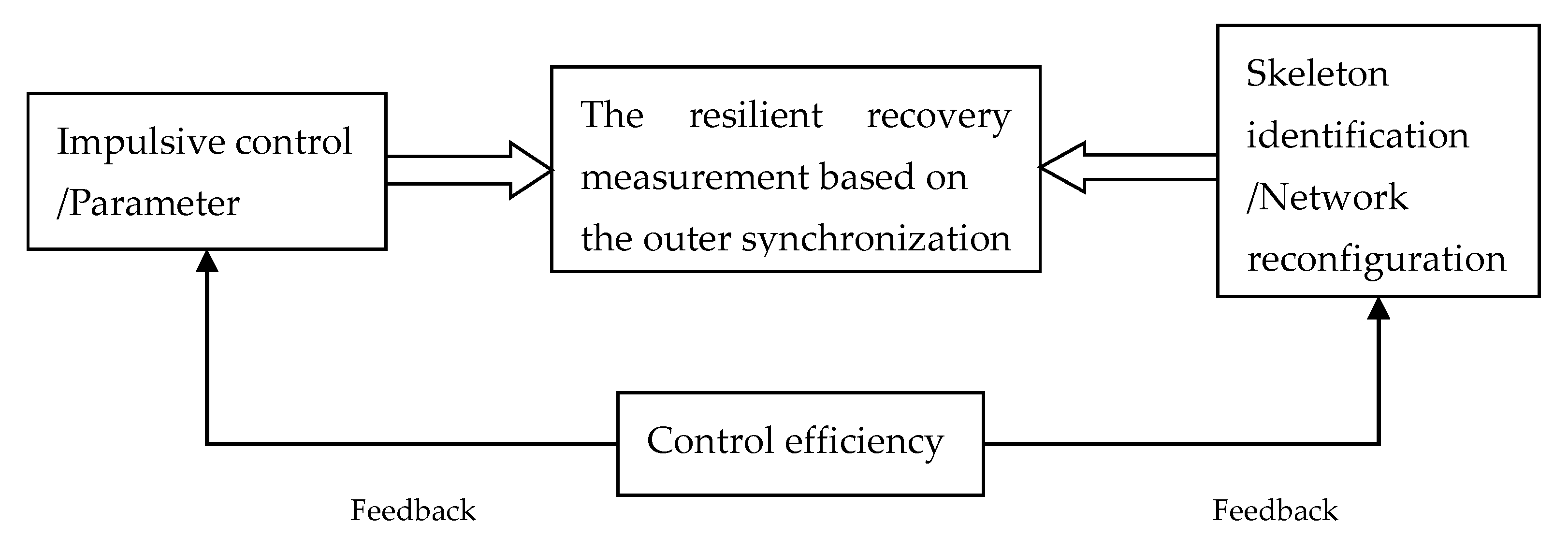
2. The Resilient Recovery of the SN Based on Outer Synchronization
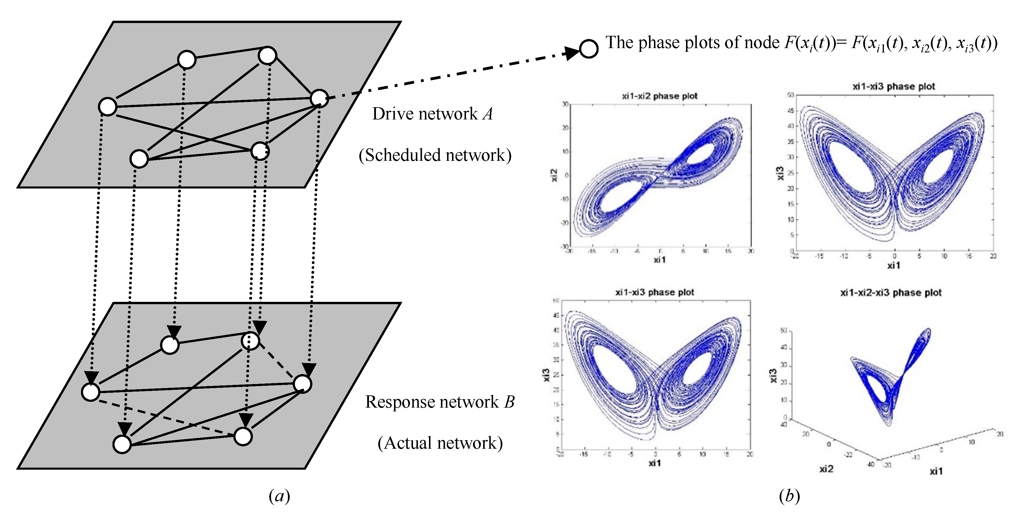
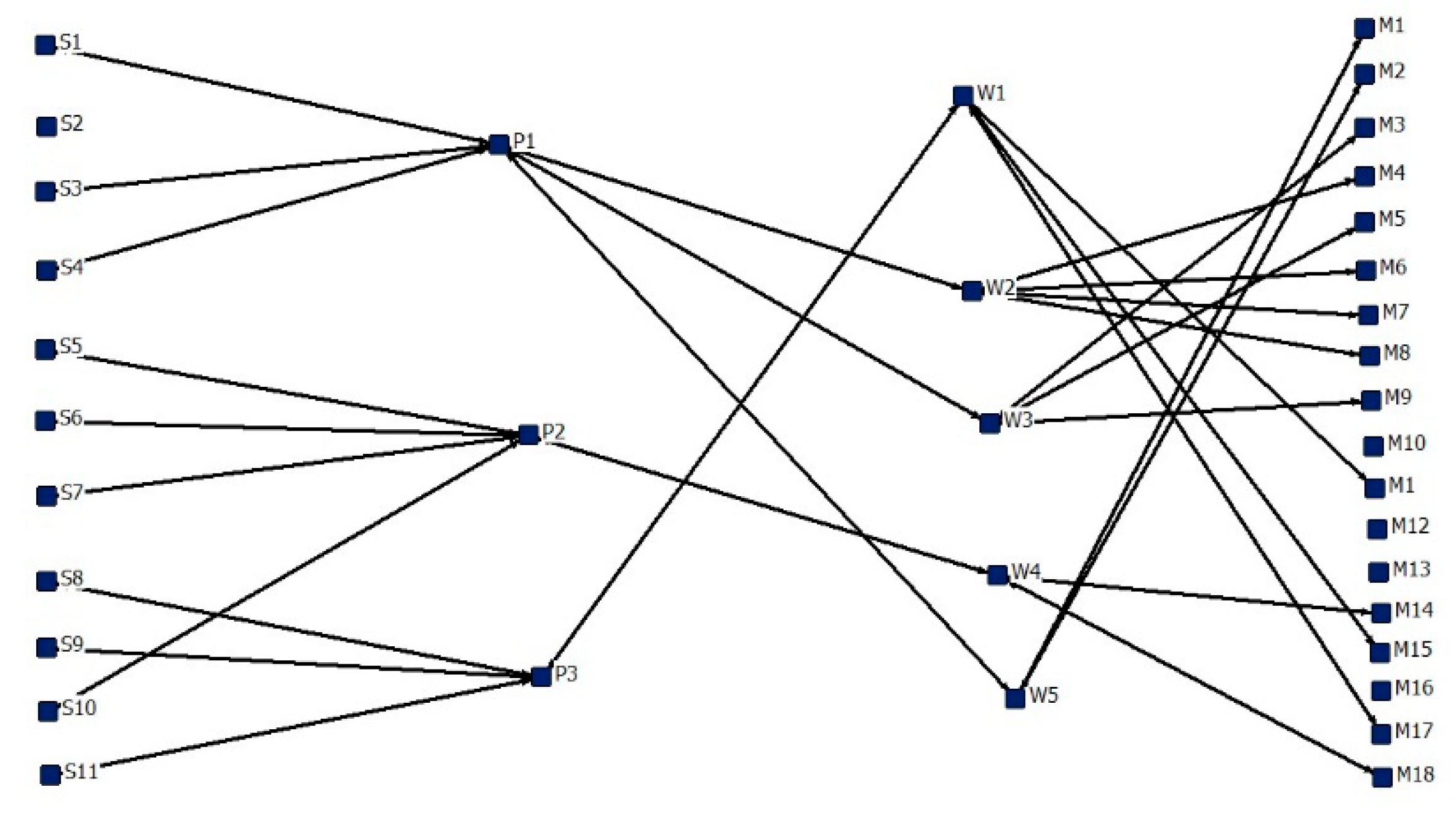
2.1. Supply Network Model
2.2. Resilient Recovery Based on Outer Synchronization
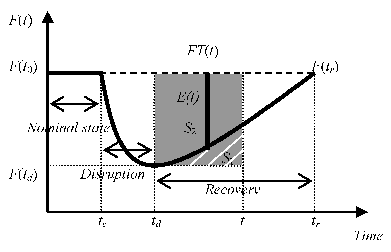
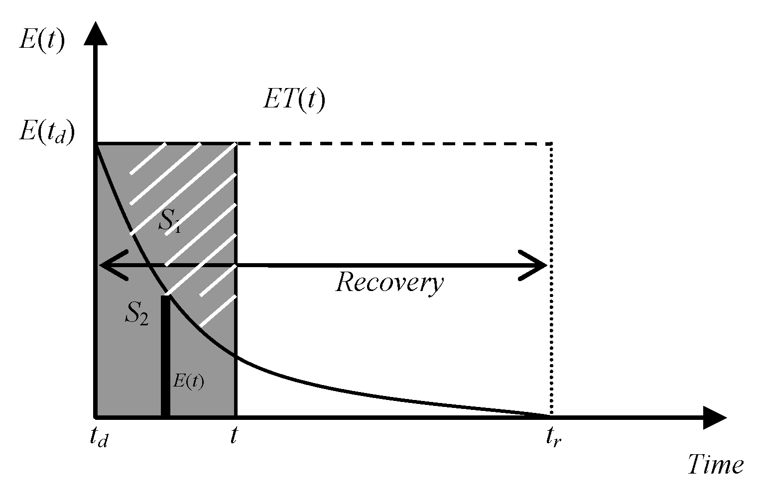
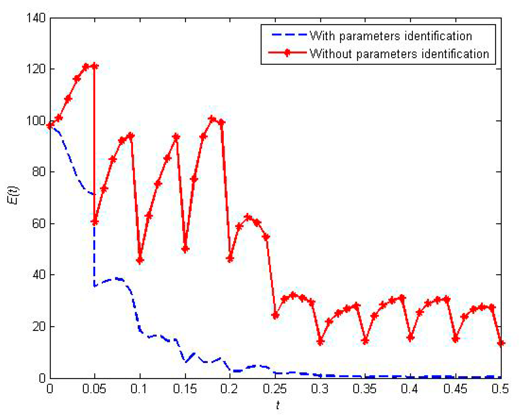
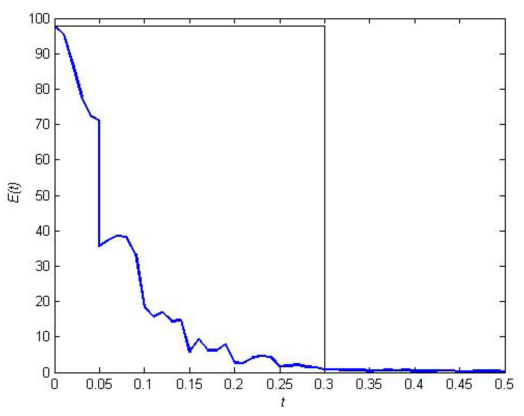
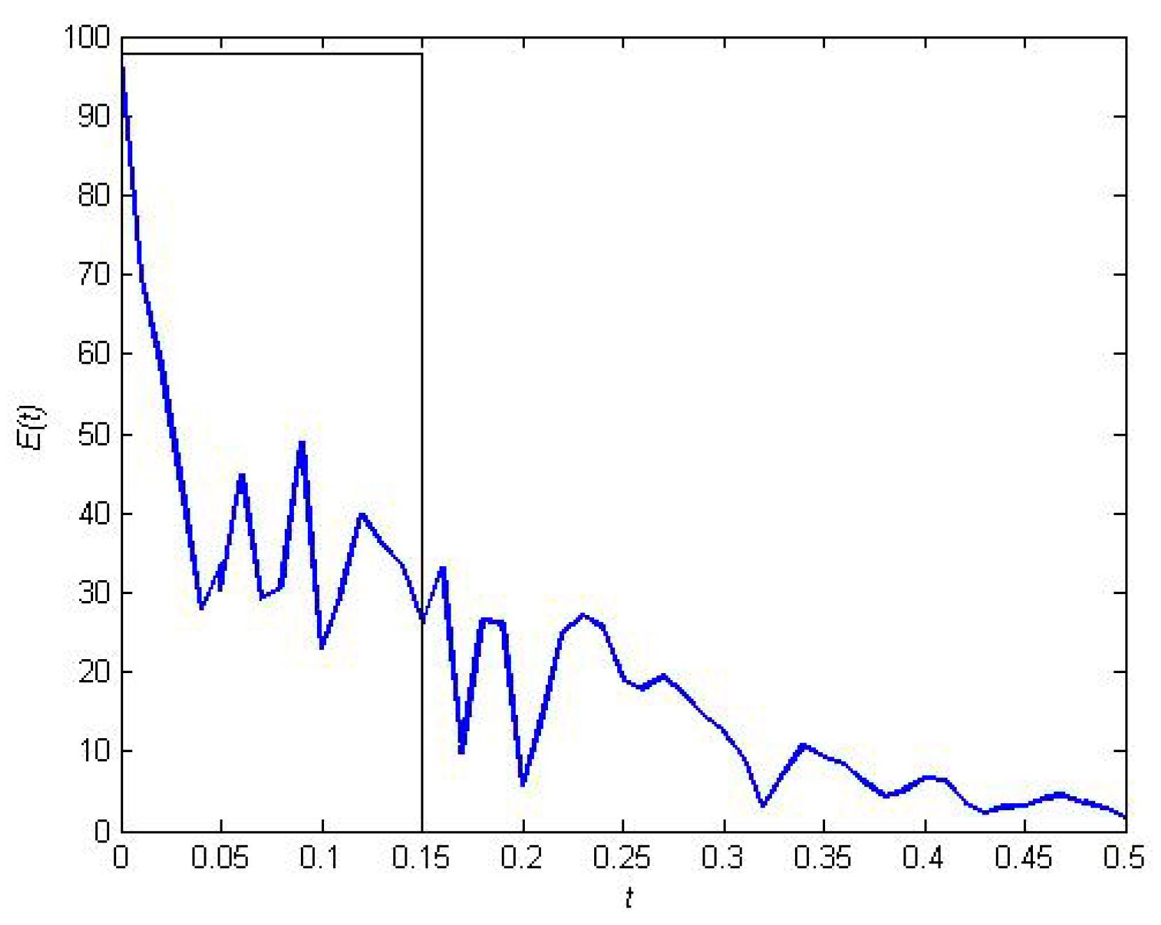
2.3. The Resilient Recovery Measurement Based on the Outer Synchronization Error
3. Design of Adaptive-Impulsive Controller
4. Application of the Method
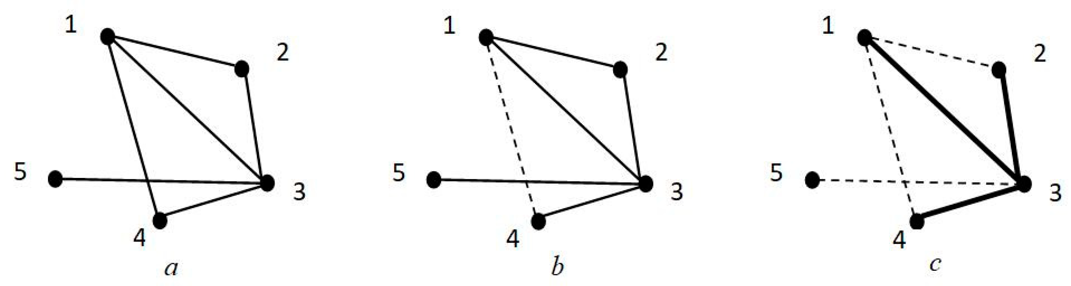
4.1. Network Skeleton Identification Forresilient Recovery
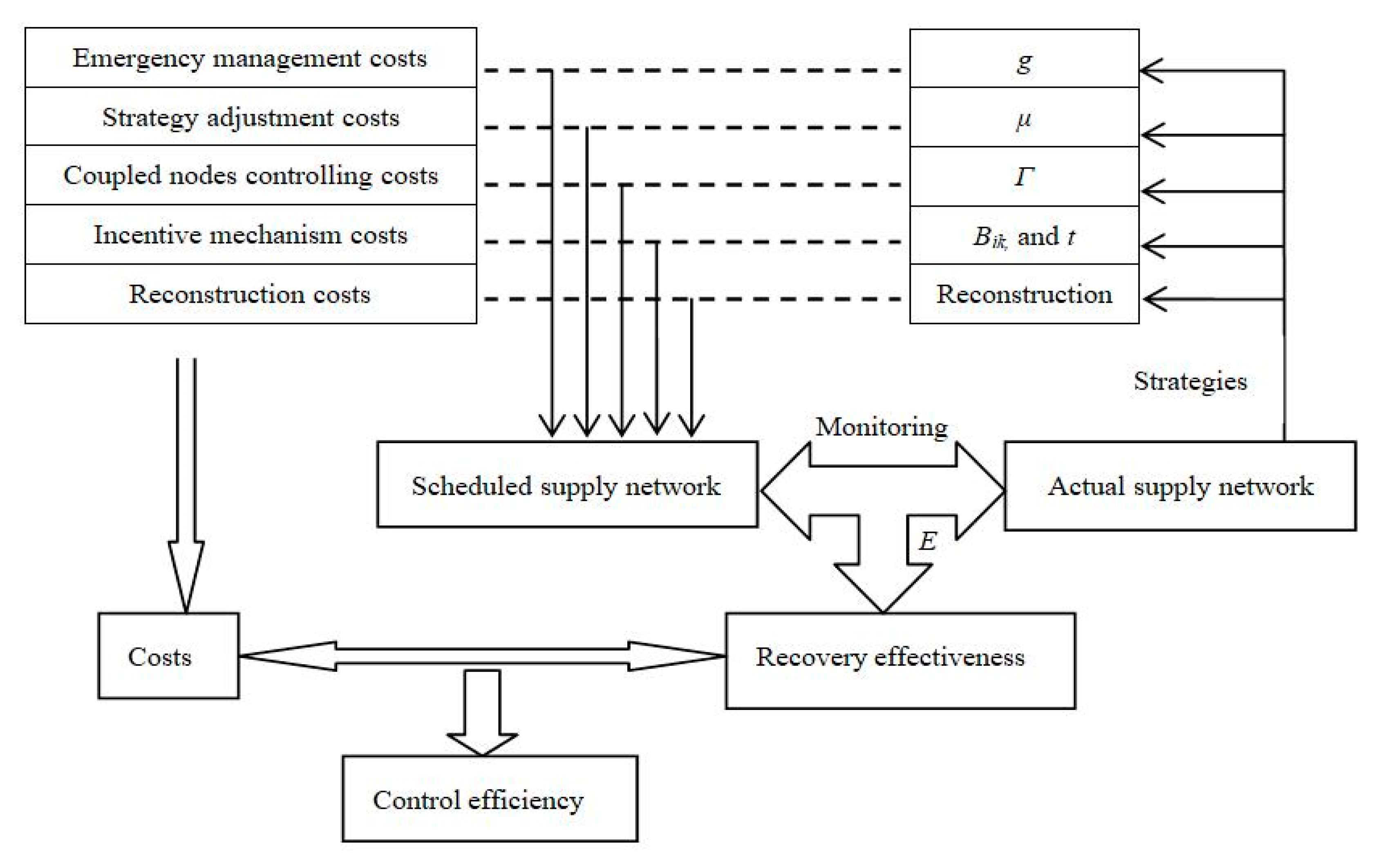
4.2. Control Efficiency Analysis
- (1)
- Emergency management costs. The parameter g shows the capability of emergency management.
- (2)
- Strategy adjustment costs. The parameter μ used to identify indicates the capability for strategy adjustment.
- (3)
- Coupled node controlling costs. The coupling relationship will be changed by the structural changes. The parameter Γ is used to control the heterogeneous coupled nodes.
- (4)
- Incentive mechanism costs. The feedback matrix Bik and pulse period t are concerned with the intensity and frequency of the incentive mechanism, respectively.
- (5)
- Reconstruction costs.
5. A Case Study in Engineering Application
5.1. The Experimental Background
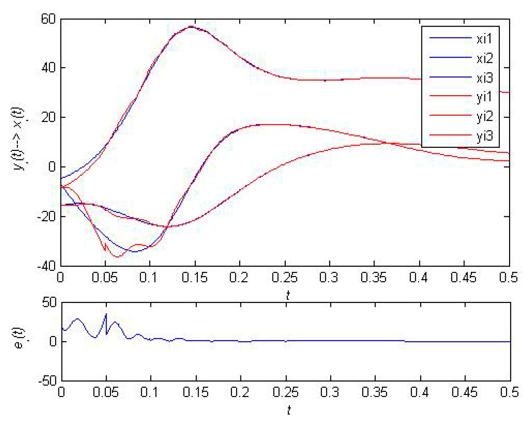
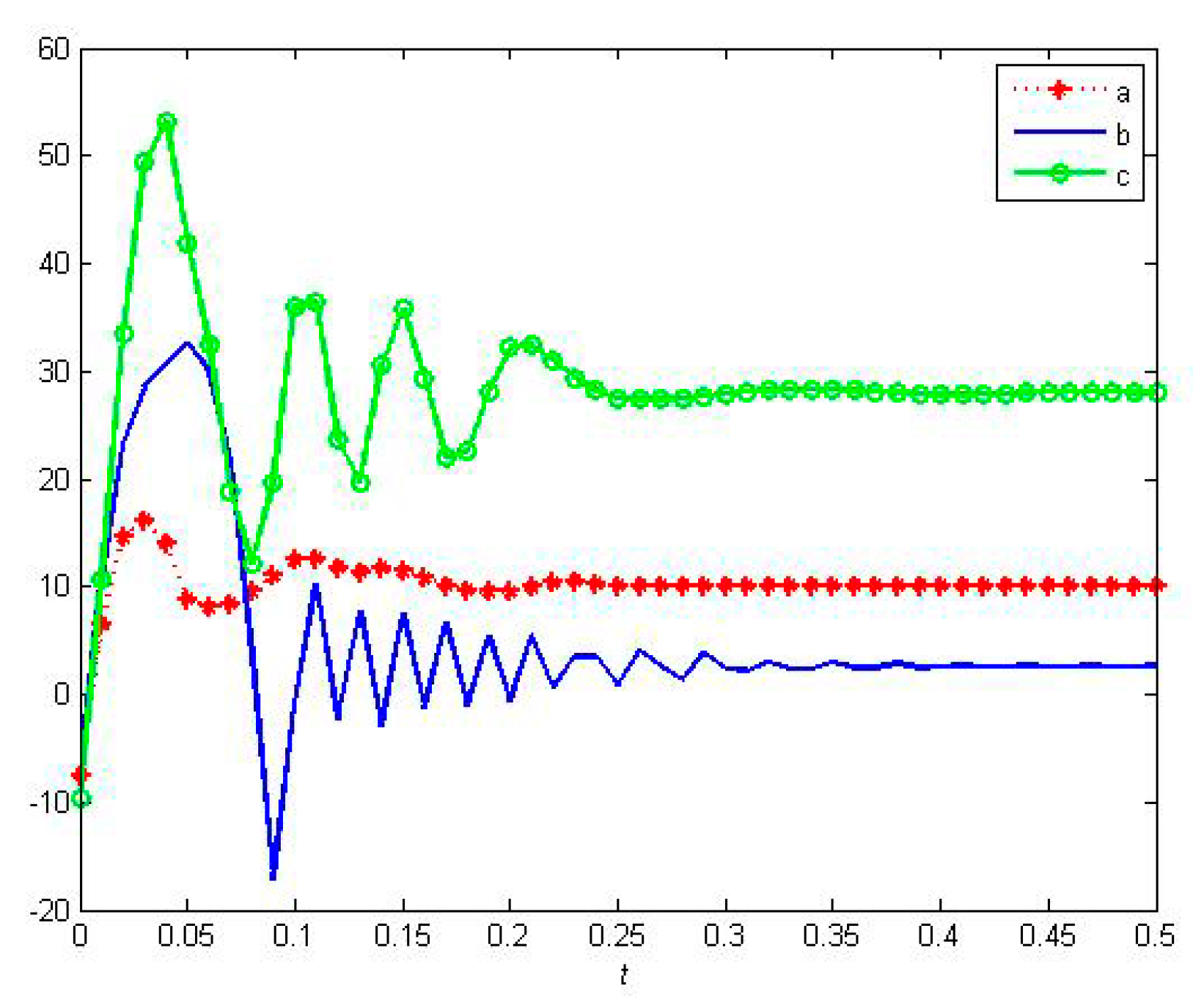
5.2. The Effectiveness of the Resilient Recovery Method based on Outer Synchronization
5.3. Backbone Identification for the Resilient Recovery of the Supply Network
5.4. Control Effect Analysis for Resilient Recovery
6. Conclusions
- (1)
- A dynamic SN model is established. The effective range of the resilient recovery method is given in Theorem 1.
- (2)
- The measurement with memory for resilient recovery is proposed by the synchronization error. This method takes into account both time and speed.
- (3)
- A greedy algorithm is designed to identify the backbone of the SN for the resilient recovery accordingly. It is very important to control the network backbone for resilient recovery.
- (4)
- Certain common control strategies correspond to the parameters in our model, such as the incentive mechanism corresponding to the intensity of impulsive control, and the strategy adjustment corresponding to the capability of parameter identification.
Author Contributions
Funding
Conflicts of Interest
References
- Subulan, K.; Baykasoğlu, A.; Özsoydan, F.B.; Taşan, A.S.; Selim, H. A case-oriented approach to a lead/acid battery closed-loop supply chain network design under risk and uncertainty. J. Manuf. Syst. 2015, 37, 340–361. [Google Scholar] [CrossRef]
- Genc, E.; Duffie, N.; Reinhart, G. Event-based supply chain early warning system for an adaptive production control. Procedia CIRP 2014, 19, 39–44. [Google Scholar] [CrossRef] [Green Version]
- Jüttner, U.; Peck, H.; Christopher, M. Supply chain risk management: Outlining an agenda for future research. Int. J. Logist. 2003, 6, 197–210. [Google Scholar] [CrossRef] [Green Version]
- Hosseini, S.; Al Khaled, A.; Sarder, M.D. A general framework for assessing system resilience using Bayesian networks: A case study of sulfuric acid manufacturer. J. Manuf. Syst. 2016, 41, 211–227. [Google Scholar] [CrossRef]
- Fiksel, J.; Polyviou, M.; Croxton, K.L.; Pettit, T.J. From risk to resilience: Learning to deal with disruption. MIT Sloan Manag. Rev. 2015, 56, 79–86. [Google Scholar]
- Fang, Y.P.; Pedroni, N.; Zio, E. Resilience-based component importance measures for critical infrastructure network systems. IEEE Trans. Rel. 2016, 65, 502–512. [Google Scholar] [CrossRef]
- Rice, J.B.; Caniato, F. Building a secure and resilient supply network. Supply Chain Manag. Rev. 2003, 7, 22–30. [Google Scholar]
- Hosseini, S.; Barker, K.; Ramirez-Marquez, J.E. A Review of Definitions and Measures of System Resilience. Reliab. Eng. Syst. Saf. 2015, 145, 47–61. [Google Scholar] [CrossRef]
- Vugrin, E.D.; Camphouse, R.C. Infrastructure resilience assessment through control design. Int. J. Crit. Infrastruct. 2011, 7, 243–260. [Google Scholar] [CrossRef]
- Liu, Y.; Slotine, J.; Barabási, A. Controllability of complex networks. Nature 2011, 473, 167–173. [Google Scholar] [CrossRef]
- Zhou, L.; Wang, C.; He, H.; Lin, Y. Time-controllable combinatorial inner synchronization and outer synchronization of anti-star networks and its application in secure communication. Commun. Nonlinear Sci. 2015, 22, 623–640. [Google Scholar] [CrossRef]
- Hohenstein, N.O.; Feisel, E.; Hartmann, E.; Giunipero, L. Research on the phenomenon of supply chain resilience: A systematic review and paths for further investigation. Int. J. Phys. Distrib. Logist. Manag. 2015, 45, 90–117. [Google Scholar] [CrossRef]
- Barker, K.; Ramirez-Marquez, J.E.; Rocco, C.M. Resilience-based network component importance measures. Reliab. Eng. Syst. Saf. 2013, 117, 89–97. [Google Scholar] [CrossRef]
- Fawcett, S.E.; Waller, M.A. Making sense out of chaos: Why theory is relevant to supply chain research. J. Bus. Logist. 2011, 32, 1–5. [Google Scholar] [CrossRef]
- Fallah, H.; Eskandari, H.; Pishvaee, M.S. Competitive closed-loop supply chain network design under uncertainty. J. Manuf. Syst. 2015, 37, 649–661. [Google Scholar] [CrossRef]
- Diabat, A.; Dehghani, E.; Jabbarzadeh, A. Incorporating location and inventory decisions into a supply chain design problem with uncertain demands and lead times. J. Manuf. Syst. 2017, 43, 139–149. [Google Scholar] [CrossRef]
- Ponta, L.; Silvano, C. Traders’ networks of interactions and structural properties of financial markets: An agent-based approach. Complexity 2018, 2018, 1–9. [Google Scholar] [CrossRef] [Green Version]
- Hearnshaw, E.J.S.; Mark, M.J.W. A complex network approach to supply chain network theory. Int. J. Oper. Prod. Manag. 2013, 33, 442–469. [Google Scholar] [CrossRef]
- Tang, H.; Chen, L.; Lu, J.A.; Chi, K.T. Adaptive synchronization between two complex networks with nonidentical topological structures. Phys. A 2008, 387, 5623–5630. [Google Scholar] [CrossRef]
- Wu, X.; Zheng, W.X.; Zhou, J. Generalized outer synchronization between complex dynamical networks. Chaos 2009, 19, 013109. [Google Scholar] [CrossRef] [Green Version]
- Lü, L.; Liu, S.; Li, G.; Zhao, G.; Gu, J.; Tian, J.; Wang, Z. Determination of configuration matrix element and outer synchronization among networks with different topologies. Phys. A 2016, 461, 833–839. [Google Scholar] [CrossRef]
- Zhang, Q.; Luo, J.; Wan, L. Parameter identification and synchronization of uncertain general complex networks via adaptive-impulsive control. Nonlinear Dyn. 2014, 71, 353–359. [Google Scholar] [CrossRef]
- Li, C.; Lü, L.; Sun, Y.; Wang, Y.; Wang, W.; Sun, A. Parameter identification and synchronization for uncertain network group with different structures. Phys. A 2016, 457, 624–631. [Google Scholar] [CrossRef]
- Li, H.L.; Jiang, Y.L.; Wang, Z.; Zhang, L.; Teng, Z. Parameter identification and adaptive–impulsive synchronization of uncertain complex networks with nonidentical topological structures. Optik 2015, 126, 5771–5776. [Google Scholar] [CrossRef]
- Wu, Z.; Fu, X. Outer synchronization between drive-response networks with nonidentical nodes and unknown parameters. Nonlinear Dyn. 2012, 69, 685–692. [Google Scholar] [CrossRef]
- Ma, X.H.; Wang, J.A. Pinning outer synchronization between two delayed complex networks with nonlinear coupling via adaptive periodically intermittent control. Neurocomputing 2016, 199, 197–203. [Google Scholar] [CrossRef]
- Liang, S.; Wu, R.; Chen, L. Adaptive pinning synchronization in fractional-order uncertain complex dynamical networks with delay. Phys. A 2015, 444, 49–62. [Google Scholar] [CrossRef]
- Sun, W.; Chen, Z.; Lü, J.; Chen, S. Outer synchronization of complex networks with delay via impulse. Nonlinear Dyn. 2012, 69, 1751–1764. [Google Scholar] [CrossRef]
- Lü, L.; Li, C.; Chen, L.; Zhao, G. New technology of synchronization for the uncertain dynamical network with the switching topology. Nonlinear Dyn. 2016, 86, 655–666. [Google Scholar] [CrossRef]
- Geng, L.; Xiao, R. Outer synchronization and parameter identification approach to the resilient recovery of supply network with uncertainty. Phys. A 2017, 482, 407–421. [Google Scholar] [CrossRef]
- Anne, K.R.; Chedjou, J.C.; Kyamakya, K. Bifurcation analysis and synchronisation issues in a three-echelon supply chain. Int. J. Logist. 2009, 12, 347–362. [Google Scholar] [CrossRef]
- Göksu, A.; Kocamaz, U.E.; Uyaroğlu, Y. Synchronization and control of chaos in supply chain management. Comput. Ind. Eng. 2015, 86, 107–115. [Google Scholar] [CrossRef]
- Kocamaz, U.E.; Taşkın, H.; Uyaroğlu, Y.; Göksu, A. Control and synchronization of chaotic supply chains using intelligent approaches. Comput. Ind. Eng. 2016, 102, 476–487. [Google Scholar] [CrossRef]
- Lei, Z.; Li, Y.; Xu, Y. Chaos synchronization of bullwhip effect in a supply chain. In Proceedings of the 13th International Conference on Management Science and Engineering, Lille, France, 5–7 October 2006; pp. 557–560. [Google Scholar]
- Ivanov, D.; Sokolov, B. Control and system-theoretic identification of the supply chain dynamics domain for planning, analysis, and adaptation of performance under uncertainty. Eur. J. Oper. Res. 2013, 224, 313–323. [Google Scholar] [CrossRef]
- Zhang, J.; Wu, Z.; Hong, L.; Xu, X. Connectivity recovery of multi-agent systems based on connecting neighbor set. Phys. A 2011, 390, 4596–4601. [Google Scholar] [CrossRef]
- Zhang, J.; Xu, X.; Hong, L.; Yan, Y. Consensus recovery of multi-agent systems subjected to failures. Int. J. Control 2012, 85, 280–286. [Google Scholar] [CrossRef]
- Wang, G.; Cao, J.; Lu, J. Outer synchronization between two nonidentical networks with circumstance noise. Phys. A 2010, 389, 1480–1488. [Google Scholar] [CrossRef]
- Tukamuhabwa, B.R.; Stevenson, M.; Busby, J.; Zorzini, M. Supply chain resilience: Definition, review and theoretical foundations for further study. Int. J. Prod. Res. 2015, 53, 5592–5623. [Google Scholar] [CrossRef]
- Cimellaro, G.P.; Reinhorn, A.M.; Bruneau, M. Framework for analytical quantification of disaster resilience. Eng. Struct. 2010, 32, 3639–3649. [Google Scholar] [CrossRef]
- Baroud, H.; Barker, K.; Ramirez-Marquez, J.E. Importance measures for inland waterway network resilience. Transport. Res. E Logist. 2014, 62, 55–67. [Google Scholar] [CrossRef]
- Wei, X.; Chen, S.; Lu, J.A.; Ning, D. Reconstruction of complex networks with delays and noise perturbation based on generalized outer synchronization. Phys. A 2016, 49, 225101. [Google Scholar] [CrossRef]
- Zhang, C.J.; Zeng, A. Network skeleton for synchronization: Identifying redundant connections. Phys. A 2014, 402, 180–185. [Google Scholar] [CrossRef] [Green Version]
- Spiegler, V.L.M.; Naim, M.M.; Wikner, J. A control engineering approach to the assessment of supply chain resilience. Int. J. Prod. Res. 2012, 50, 6162–6187. [Google Scholar] [CrossRef] [Green Version]
- Cardoso, S.R.; Barbosa-Póvoa, A.P.; Relvas, S.; Novais, A.Q. Resilience metrics in the assessment of complex supply-chains performance operating under demand uncertainty. Omega Int. J. Manag. 2015, 56, 53–73. [Google Scholar] [CrossRef]


| Denotation | Definition |
|---|---|
| xi | The status of node i |
| xi1 | Demand quantities for ordering |
| xi2 | Supply quantities for distribution |
| xi3 | Inventory for production |
| m | The dissatisfaction of ordering |
| r | Information distortion |
| b | The coefficients of safety stock |
| Type | S | P | W | M | m | r | b | Γ |
|---|---|---|---|---|---|---|---|---|
| values | 11 | 3 | 5 | 18 | 10 | 28 | 2.6 | diag(5, 5, 5) |
| 1 | 2 | 3 | 4 | 5 | 6 | 7 | 8 | 9 |
| M8-W3 | W1-P2 | W3-P2 | M3-W5 | W2-P2 | W3-P3 | M16-W1 | M9-W2 | W2-P3 |
| 0.5583 | 0.5585 | 0.5582 | 0.5582 | 0.5579 | 0.5581 | 0.5585 | 0.5582 | 0.5579 |
| 10 | 11 | 12 | 13 | 14 | 15 | 16 | 17 | 18 |
| P1-S2 | M16-W3 | M15-W3 | M12-W3 | P3-S10 | M10-W1 | M13-W4 | W4-P3 | W5-P3 |
| 0.5577 | 0.5573 | 0.5559 | 0.5564 | 0.5552 | 0.5524 | 0.5499 | 0.5482 | 0.5456 |
| Network Structure | Remove Links | R(0.3) | |
|---|---|---|---|
| Backbone | 18 links, as in Table 2 | 0.7127 | |
| Case 1 | Network 1 | W3-M3, W3-M5, W3-P1, W1-M11, W1-M17, W1-P3 | 0.7132 |
| Network 2 | W3-M8, W3-M12, W3-P2, W1-M10, W1-M16, W1-P2 | 0.7250 | |
| Case 2 | Network 3 | P2-S5, P2-S6, P2-W4, W2-P1, W2-P6, W2-M8 | 0.7205 |
| Network 4 | P3-S10, P3-W2, P3-W3, W2-P2, W2-M9, W3-M12 | 0.7236 | |
| Case 3 | Network 5 | W5-M1, W5-M2, W5-P1, W1-M11, W1-M15, W1-P3 | 0.7073 |
| Network 6 | W5-M3, W5-P3, P3-W4, P3-W3, P3-W2, P2-W1 | 0.7253 |
| Scenario 1 | Strategy | Strategy Parameter | Cost Parameter | Cost | R(0.3) | RC(0.3) |
|---|---|---|---|---|---|---|
| Strategy 1 | Emergency management | Δg = 1 | Kg = 0.15 | C = C0 + Kg*Δg = 6.10 | 0.7509 | 0.1231 |
| Strategy 2 | Strategy adjustment | Δμ = 1 | Kμ = 0.1 | C = C0 + Kμ*Δμ = 6.05 | 0.7091 | 0.1172 |
| Strategy 3 | Coupled node control | ΔΓ = 1 | KΓ = 0.1 | C = C0 = +KΓ*ΔΓ = 6.05 | 0.7075 | 0.1169 |
| Strategy 4 | Incentive mechanism | ΔBik, = 0.1 | KBik, = 1 | C = C0 = +KBik, *ΔBik, *T/t = 6.95 | 0.7264 | 0.1045 |
| Strategy 5 | Reconstruction | ΔRC = W1-P3 | KRC = 1 | C = C0 + KRC *ΔRC = 6.95 | 0.7086 | 0.1018 |
| ΔRC = W1-P2 | KRC = 1 | C = C0 + KRC *ΔRC = 6.95 | 0.7080 | 0.1017 |
| Strategy | Strategy Parameter | Cost Parameter | Cost | R(0.3) | RC(0.3) | |
|---|---|---|---|---|---|---|
| Strategy 4 | Incentive mechanism | ΔBik, = 0.1 | KBik, = 0.5 | C = C0= +KBik, *ΔBik, *T/t = 3.95 | 0.7264 | 0.1839 |
© 2019 by the authors. Licensee MDPI, Basel, Switzerland. This article is an open access article distributed under the terms and conditions of the Creative Commons Attribution (CC BY) license (http://creativecommons.org/licenses/by/4.0/).
Share and Cite
Geng, L.; Xiao, R. Control and Backbone Identification for the Resilient Recovery of a Supply Network Utilizing Outer Synchronization. Appl. Sci. 2020, 10, 313. https://doi.org/10.3390/app10010313
Geng L, Xiao R. Control and Backbone Identification for the Resilient Recovery of a Supply Network Utilizing Outer Synchronization. Applied Sciences. 2020; 10(1):313. https://doi.org/10.3390/app10010313
Chicago/Turabian StyleGeng, Liang, and Renbin Xiao. 2020. "Control and Backbone Identification for the Resilient Recovery of a Supply Network Utilizing Outer Synchronization" Applied Sciences 10, no. 1: 313. https://doi.org/10.3390/app10010313
APA StyleGeng, L., & Xiao, R. (2020). Control and Backbone Identification for the Resilient Recovery of a Supply Network Utilizing Outer Synchronization. Applied Sciences, 10(1), 313. https://doi.org/10.3390/app10010313