Concentration Quantification of Oil Samples by Three-Dimensional Concentration-Emission Matrix (CEM) Spectroscopy

Abstract

Developing fast and accurate fluorescence detection technology of oil spill is significant for quantitative analysis in unexpected oil spill events. As the oil sample concentration increases, the fluorescence spectrum produces red-shift behavior, which seriously affects the quantitative detection of concentration. In this work, a three-dimensional concentration-emission matrix (CEM) was constructed by using a series of emission spectra with different levels of concentration at the excitation wavelength of 266 nm. The database is the interpolated CEM of six samples using bicubic interpolation in the concentration dimension. With matrix similarity matching, the database was used to achieve quantification of the concentration of oil samples. The recovery rates of prediction for test samples and weathering samples of six oil samples were between 86.8% and 116.11%, with relative errors of predictions ranging from 2.09% to 15.2%. The results show that this method can provide accurate quantitative determination of the concentration of different oil samples.

1. Introduction

In recent years, oil spills have occurred frequently, causing enormous damage to the marine environment and the socio-economy. Therefore, it is of considerable significance for emergency treatment of oil spill accidents to quickly determine the source and total amount of oil spills by using accurate qualitative and quantitative analysis. However, the oil components and their changes are complicated. The ability to promptly discriminate oil species and determine the oil concentrations in seawater accordingly is a critical issue for current research.

At present, conventional methods to achieve this include gas chromatography-mass spectroscopy (GC-MS), gas chromatography-flame ionization detection (GC-FID), and so on [1,2,3,4,5,6]. With the advantages of high sensitivity, good selectivity, and high analytical efficiency, these methods have been considered as the most reliable methods for oil spill analysis. However, these instruments are expensive, and the pre-treatment of samples is complicated. Therefore, the above techniques are challenging to use to meet online monitoring requirements.

Due to the presence of polycyclic aromatic compounds in petroleum, most petroleum can emit fluorescence. Fluorescence detection technologies can be applied to oil monitoring. The main fluorescence methods include Synchronization Fluorescence Spectrum (SFS) [7,8,9], Excitation Emission Matrix (EEM) [10], and Time-Resolved Fluorescence (TRF) [11,12]. Some researchers studied the rapid measurement of oil concentration in water by using three-dimensional fluorescence spectroscopy and PARAFAC algorithm with the interference of a variation of dissolved organic matter [13]. The fluorescence and light scattering combined with artificial neural networks were used to quickly determine the total oil concentration in water [14]. Fluorescence spectroscopy does not destroy the sample structure and does not require pretreatment of the sample. The measurement process is convenient and has high sensitivity and accuracy.

Fluorescence intensity is liner with oil concentration in water only when the sample concentration is low. Therefore, conventional fluorescence technology can be used to dilute the sample to a linear concentration range for measurement. However, oils contain a variety of Polycyclic Aromatic Hydrocarbons (PAHs) components. When the oil concentration is high, the lower ring PAHs will produce fluorescence quenching, resulting in the remaining fluorescent information only representing the higher ring PAHs. Some researchers have found a phenomenon where the spectra are reliant on the concentration of multi-PAHs, which was called “red-shift behavior” [15,16]. Thus, fluorescence spectra of one certain concentration level are difficult to use to fully represent the fluorescence characteristics of oil samples. It is hard to judge whether the oil concentration or the oil species causes a change in spectral shape.

To address this problem, a three-dimension concentration-emission matrix (CEM) spectrum was constructed by obtaining the fluorescence emission spectra at 10 series of concentrations. The CEM has been interpolated in the concentration interval and the spectral matrix of the test samples or weathering samples are compared to the database of interpolated CEM generated above. The maximum similarity coefficient (more than 0.9) means the closest matching species and the corresponding concentrations are the concentration of the sample. The quantitative results were evaluated based on recovery rate and relative error of prediction.

2. Experimental Procedure

2.1. Samples and Reagents

Six different types of oils: 0^#diesel, crude oil, heavy oil, 92^#gasoline, shell helix 10w-40, and motor oil 20w-40 were selected to analyze the quantification accuracy of concentration. The isopropanol was chosen as the extracting agent due to its low fluorescence efficiency. The oil sample was weighted by electronic balance and dissolved in isopropanol, which was placed in an ultrasonic oscillator to be fully dissolved. After waiting for 30 min, the supernatant was taken as the stock solution with a concentration of 5000 ppm of the oil sample. The concentrations of working solutions with a serial of concentrations (1.2 ppm, 2.4 ppm, 4.9 ppm, 9.8 ppm, 19.5 ppm, 39 ppm, 78 ppm, 156 ppm, 312 ppm, 625 ppm, respectively) was prepared by diluting the stock solutions. A series of test samples (5 ppm, 100 ppm, 200 ppm, 400 ppm, 600 ppm) was prepared by diluting the stock solutions.

2.2. Apparatus

Fluorescence measurement was carried out with a Hitachi F-7000 spectrofluorometer. The excitation-emission matrices for three-dimension fluorescence spectra of each sample were recorded with the excitation wavelengths EX in range of 250–450 nm at a 2 nm interval, and emission wavelength EM 260–550 nm were recorded at a 2 nm interval. EEMSCAT [17] was used to remove Raman scattering and Raleigh scattering in the MATLAB environment.

2.3. Weathering Experiments

In order to verify the quantitative accuracy of the method under different conditions, the weathering influence was taken into consideration in the experiments. A seven days weathering experiment was designed. The oil samples were subjected to weathering by placing 2 cm thick oil film in a beaker, placed in outdoor conditions for seven days to receive natural solar radiation. The oil samples (0#diesel, crude oil, heavy oil, shell helix 10w-40, and motor oil 20w-40) weathered for one day, two days, five days and seven days were prepared as weathering stock solutions 5000 ppm-1d, 5000 ppm-2d, 5000 ppm-5d, and 5000 ppm-7d, respectively. Due to the volatility of 92#gasoline, the sample weathered for two days was prepared into 5000ppm-1d and 5000ppm-2d stock solutions.

3. Results and Discussion

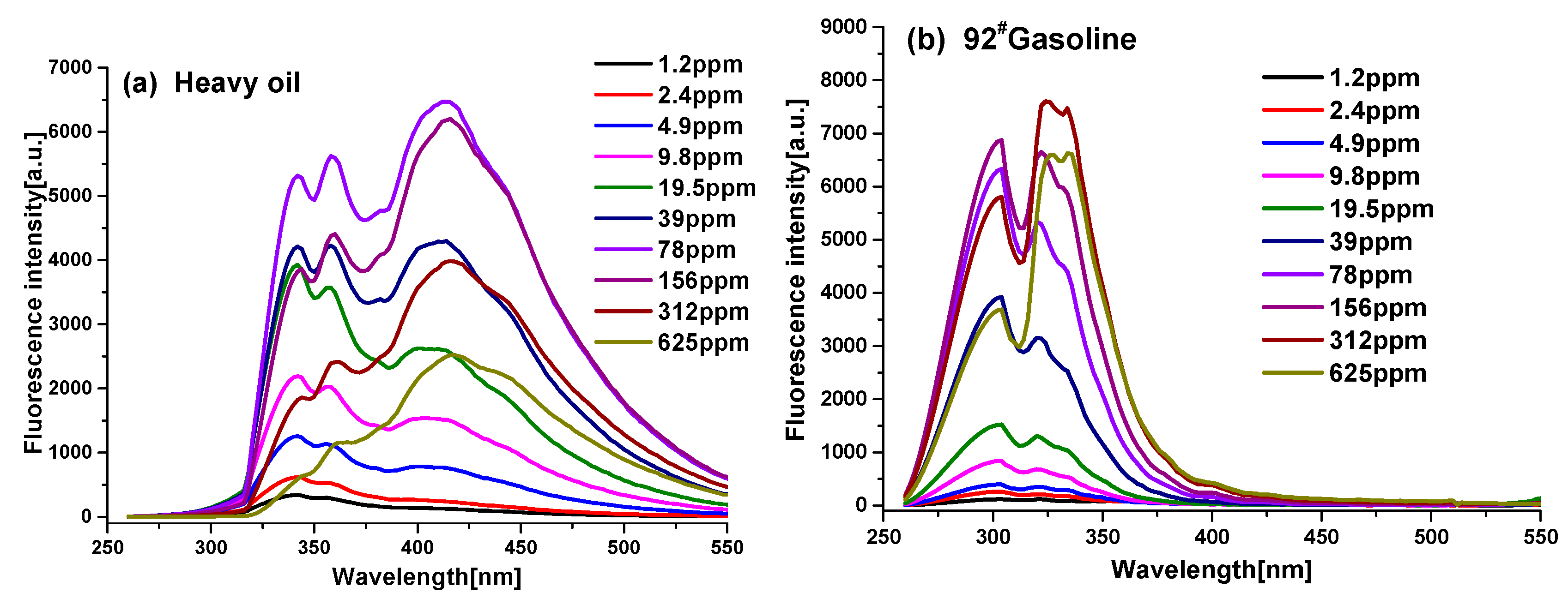
3.1. Fluorescence Spectral Properties of Oils at Different Concentrations

The Excitation-Emission-Matrix (EEM) fluorescence spectrum can be generated by collecting several emission spectra at series excitation wavelengths and combining them. It can clearly show the variation of fluorescence characteristics with the concentration, such as the number of peaks, peak location, peak intensities, and peak shapes. Take crude oil as an example. The EEM fluorescence spectra obtained at the concentrations of 1.2 ppm, 19.5 ppm, 78 ppm, 156 ppm, 312 ppm, 625 ppm are shown in Figure 1.

It was clear that the main fluorescence center was at the ${\mathsf{\lambda }}_{ex}/{\mathsf{\lambda }}_{em}$ of 295 nm/342 nm in the low concentration of 1.2 ppm and the fluorescence characteristics of low-ring PAHs were exhibited. As the oil concentration increased, the fluorescence peak gradually moved toward the long wavelength and the fluorescence maxima located at ${\mathsf{\lambda }}_{ex}/{\mathsf{\lambda }}_{em}$ of 275 nm/420 nm. When the concentration increased to 625 ppm, a new fluorescent peak appeared at the ${\mathsf{\lambda }}_{ex}/{\mathsf{\lambda }}_{em}$ of 312 nm/420 nm and the other fluorescence peak was still located at the ${\mathsf{\lambda }}_{ex}/{\mathsf{\lambda }}_{em}$ of 275 nm/420 nm, which represents the fluorescence characteristics of high-ring PAHs. The reason why the spectrum changes with concentration was that the oil sample contained a variety of aromatic compounds, which cause self-absorption, light attenuation, collision quenching, and molecular aggregation with increased concentration. The results demonstrate that the fluorescence spectrum of the oil has a “red-shift” behavior as the oil concentration increases, which needs to be considered in quantitative measurement.

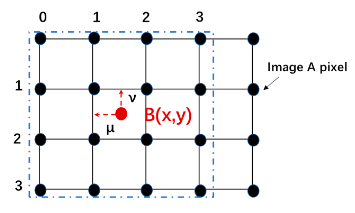
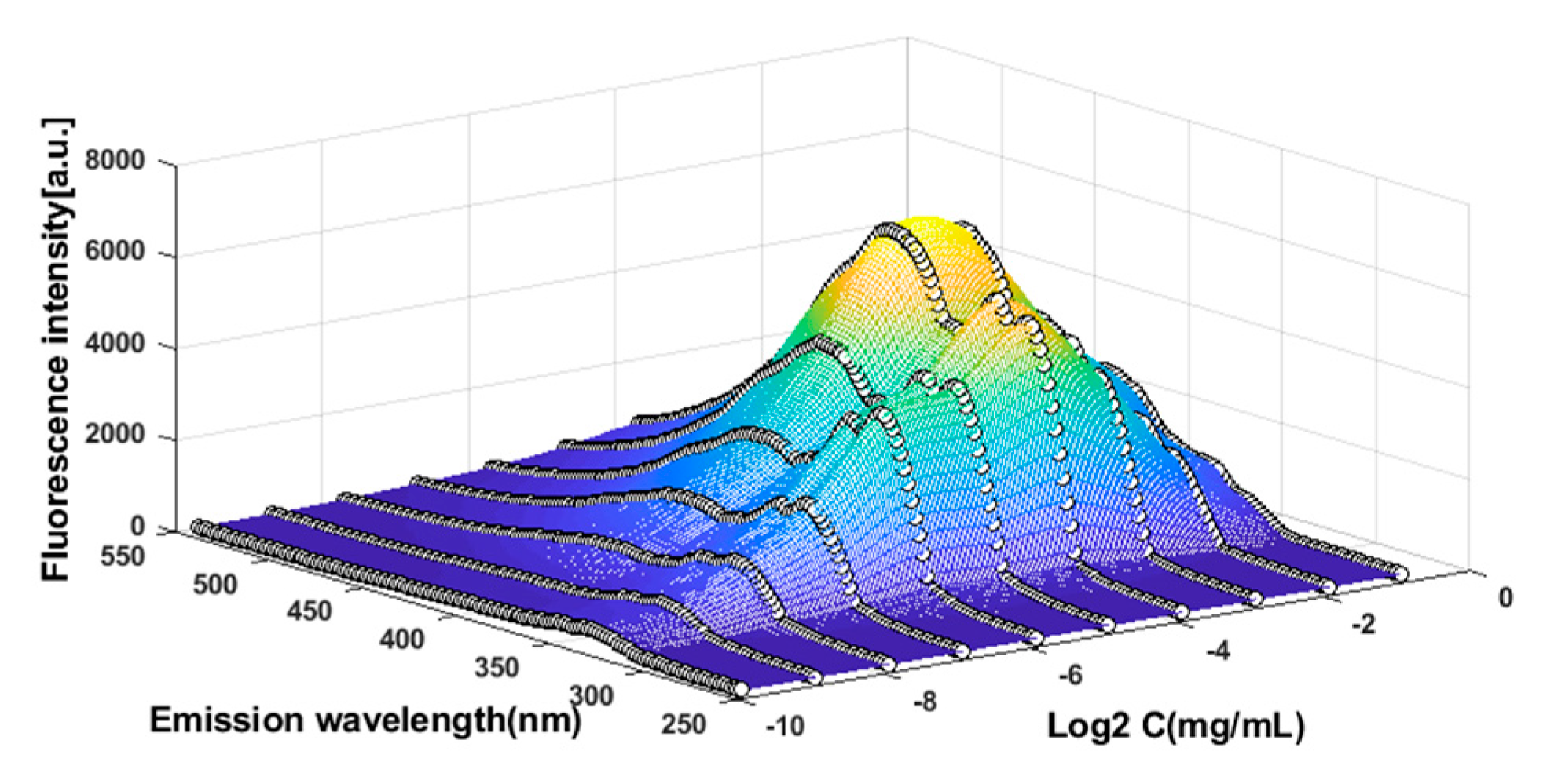
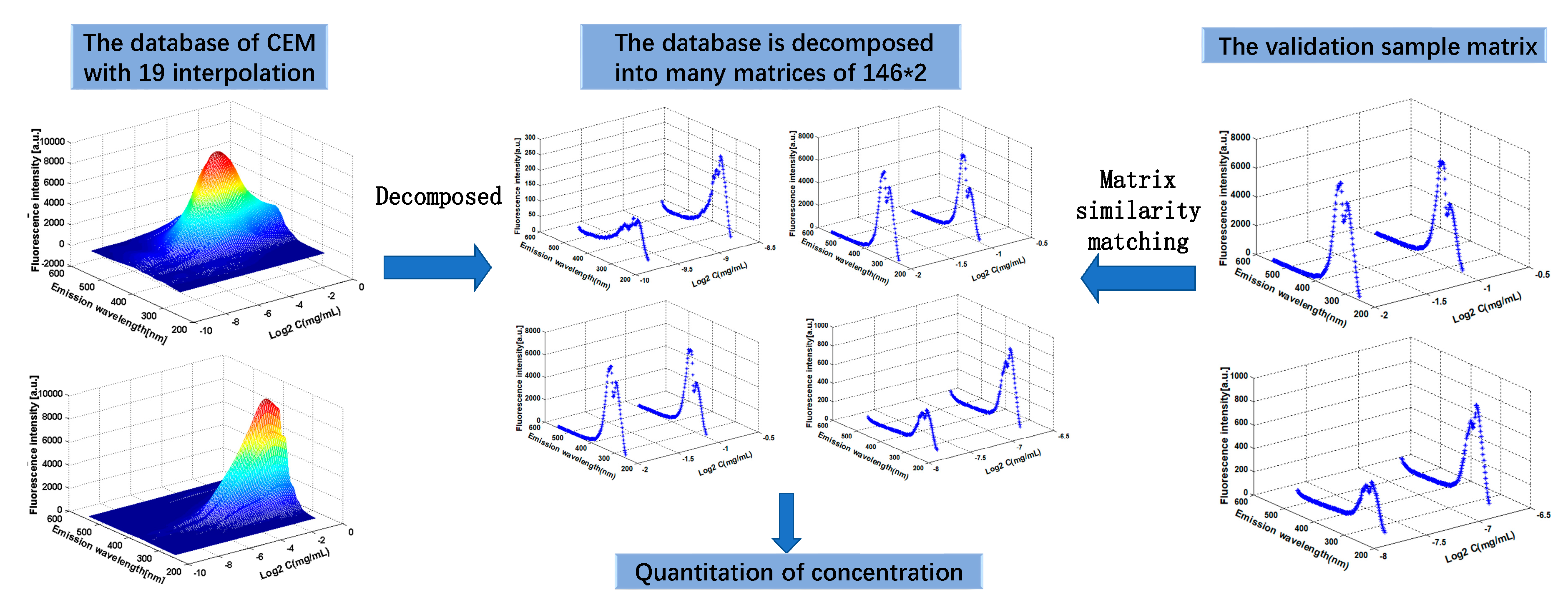
3.2. The Construction of CEM Spectra

The emission spectrum at the optimum excitation wavelength was selected to represent the spectral characteristics of the sample, which was used as the simplified data of the EEM spectrum. The emission spectra at different concentrations were obtained to form the Three-dimensional concentration-emission matrix (CEM).

The effective excitation wavelengths of oils ranged from 200 nm to 400 nm. For the determination of oils in water, the far ultraviolet (less than 290 nm) was the most widely used wavelength. In this work, the emission spectrum at the excitation wavelength of 266 nm was selected as the characteristic spectrum of the oil. It can be seen that the fluorescence intensities of two oils increased first and then decreased with an increasing concentration. Moreover, the spectra of different oils showed different characteristics as the concentration increased. Figure 2 shows the emission spectra of heavy oil and 92^#gasoline measured over a broad concentration range (1.2 ppm–625 ppm).

These spectra were measured in a wide range of concentrations, leaving considerably long intervals, which causes the CEM to have discrete spectra in the concentration dimension. In order to predict the concentration of oil, a good solution was to use the bicubic interpolation to smooth the CEM spectrum.

Bicubic interpolation is a new technique for resampling discrete data that can achieve the effect of magnifying images and obtaining high-resolution images [18]. The principle of bicubic interpolation is shown in Figure 3. The bicubic interpolation not only considers the influence of four directly adjacent points but calculates the influence factors of 16 points around the sampling point for interpolation. The basic function W(x) of Bicubic was:

$$\mathrm{W}\left(\mathrm{x}\right)=\{\begin{array}{ll}(a+2){\left|x\right|}^3-(a+3){\left|x\right|}^2+1& \mathrm{for} \left|x\right| \le 1\\ a{\left|x\right|}^3-5a{\left|x\right|}^2+8a\left|x\right|-4a& \mathrm{for} 1<\left|x\right|<2\\ 0& \mathrm{otherwise}\end{array}.$$

(1)

The horizontal and vertical distances from the interpolation B(x, y) to 16 pixels are $K_{im}$ and $K_{jn}$:

$$\begin{gathered} K_{i0}=1+\mu ;K_{i1}=\mu ;K_{i2}=1-\mu ;K_{i3}=2-\mu ; \\ {K}_{j0}=1+\nu ; K_{j1}=\nu ;K_{j2}=1-\nu ;K_{j3}=2-\nu . \end{gathered}$$

(2)

The weight coefficient is:

$$a_{mn}=W\left(K_{im}\right)W\left(K_{jn}\right)$$

Finally, the interpolated image is:

$$\mathrm{B}\left(\mathrm{x},\mathrm{y}\right)={\displaystyle \sum }_{i = 0}^3{\displaystyle \sum }_{j = 0}^3{a}_{ij}A\left(x_i, y_j\right)$$

(3)

where A is the original image point, B is the interpolated image point, $a_{ij}$ represents the weight parameter, and i, j represent the horizontal and vertical coordinates, respectively.

To improve the quantitative accuracy of concentration, 19 computing spectra were interpolated in each concentration interval. The spectrum obtained by bicubic interpolation of heavy oil is shown in Figure 4. The X-axis is the logarithmic form of concentration (mg/mL), Y-axis is the emission wavelength (nm), Z-axis is the fluorescence intensity.

The database of interpolation CEM was constructed by measuring the fluorescence spectra of oil samples at different concentrations. Figure 5 shows the interpolation CEM of six kinds of oils using bicubic interpolation.

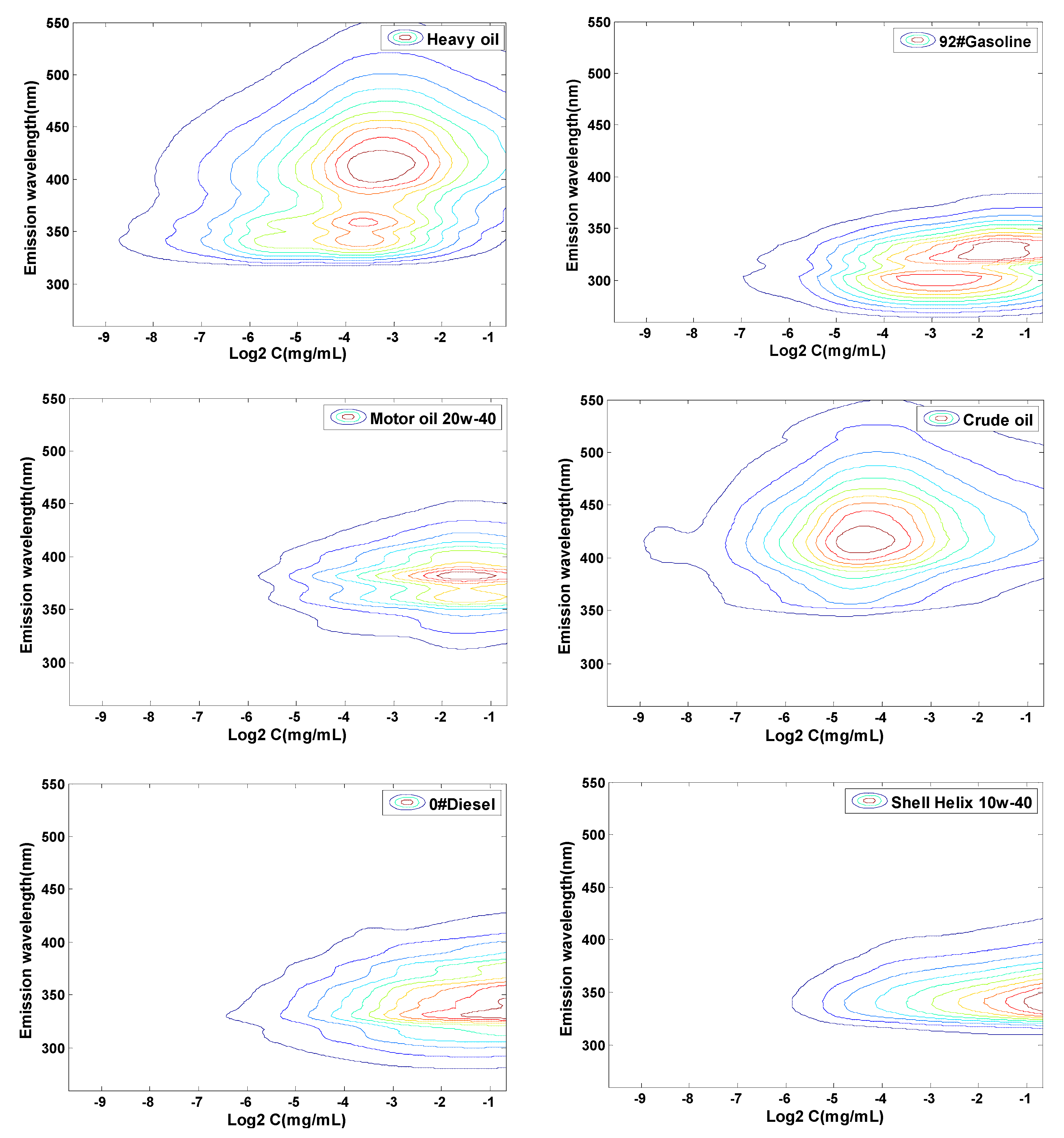
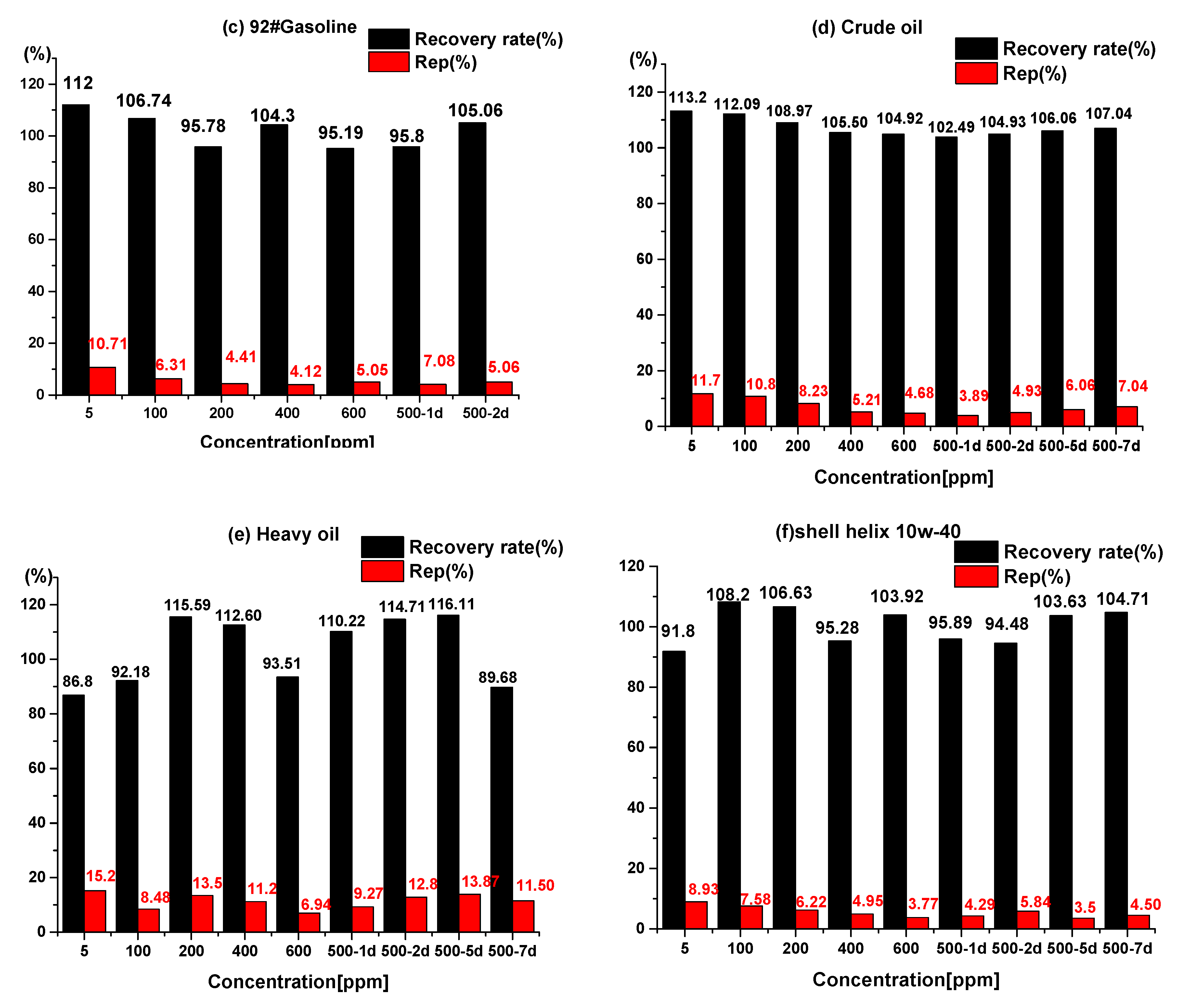
3.3. Quantitative Analysis of Concentration Based on CEM

The test samples with a series of concentration and the weathering samples in seven days were used to analyze the quantitative accuracy of the method. In order to calculate the concentrations of the test samples and weathering samples, the processing occurred as follows:

Firstly, the emission spectrum matrix of the initial concentration of test samples was 146 × 1, and the emission spectrum of concentration diluted by half was 146 × 1. The spectra of the two concentrations were combined to form test sample spectral matrix of 146 × 2. The spectral processing of weathering samples was similar to the above method.

Secondly, the database of interpolated CEM generated above was decomposed into a series of matrices (146 × 2), with one column representing the spectrum of the n-th column and the other column representing the spectrum of the (n + 21) column in the concentration direction.

Finally, the similarity between the decomposed matrices and the test matrices was used to calculate the concentration of test samples and weathering samples. The maximum similarity coefficient (r) means that the concentration was the predicted concentration of the test sample or weathering sample. The quantitative principle is shown in Figure 6.

The similarity coefficient (r) of the matrix [19] is:

$$\mathrm{r} =\frac{{{\displaystyle \sum }}_m^{}{{\displaystyle \sum }}_n^{}\left(A_{mn} - \overline{A}\right)\left(\left(B_{mn} - \overline{B}\right)\right)}{\sqrt{({{\displaystyle \sum }}_m^{}{{\displaystyle \sum }}_n^{}{\left(A_{mn} -\overline{ A}\right)}^2)({{\displaystyle \sum }}_m^{}{{\displaystyle \sum }}_n^{}{\left(B_{mn} -\overline{ B}\right)}^2)}}$$

(4)

where $\overline{A}$ is the mean (mean (A)), and $\overline{B}$ is the mean (mean (B)).

The accuracy of the quantitation of the six oils was evaluated based on two indexes: recovery rate (R) [20] and relative error of prediction (Rep) [21]. The formula is as follows:

$${\mathrm{R}}_i = \frac{\widehat{C_i}}{C_i} * 100\%$$

(5)

$$\mathrm{REP}=\frac{\left|\widehat{C_i} - C_i\right|}{C_i} * 100\%$$

(6)

where $\widehat{C_i}$ and $C_i$ are the predicted concentration and the actual concentration in the i-th unknown sample.

Based on the interpolated CEM of six oil samples, the concentrations of test samples and weathering samples could be predicted. Figure 7 shows the predicted results of test samples with a series of concentration and weathering samples.

It can be seen that the recovery rates of predictions for test samples and weathering samples of six oils were between 86.8% to 116.11%, and the relative errors of predictions ranged from 2.09% to 15.2%. The results demonstrate that accurate quantification of the concentration of oils can be effectively realized based on CEM spectra and similarity analysis.

4. Conclusions

In this work, the feasibility of quantifying the concentrations of oil samples based on three-dimensional concentration-emission matrix (CEM) spectra, which were constructed by the emission spectra of 10 concentrations and were supplemented by the spectral change information between adjacent concentrations, was studied. The results show that the predicted recovery rates for test samples of six oil samples are between 86.8% and 115.59%, and the relative errors are in the range of 2.09–15.2%. The predicted recovery rates for weathering samples are in the range of 89.68–116.11%, and the relative errors range from 2.47% to 13.87%. The CEM spectra, interpolated in concentration dimension via a bicubic interpolation and combined with matrix similarity matching, can predict the concentration of test samples and weathering samples with good quantitative accuracy.

References

1. Liu, Y.; He, J.; Song, C. Oil Fingerprinting by Three-Dimensional (3D) Fluorescence Spectroscopy and Gas Chromatography–Mass Spectrometry (GC–MS). Environ. Forensics 2009, 10, 324–330. [Google Scholar] [CrossRef]
2. Taki, M.; Asahara, T.; Mandai, Y.; Uno, T.; Nagai, M. Discriminatory Analysis of Crude Oils Using Biomarkers. Energy Fuels 2009, 23, 5003–5011. [Google Scholar] [CrossRef]
3. Matysik, S.; Schmitz, G. Application of gas chromatography–triple quadrupole mass spectrometry to the determination of sterol components in biological samples in consideration of the ionization mode. Biochimie 2013, 95, 489–495. [Google Scholar] [CrossRef] [PubMed]
4. Shun, P.; Zhou, Q.; Guang, M.; Wang, X.; Zhao, Y.; Cao, L. Fingerprint analysis of polycyclic aromatic hydrocarbons in crude oil by internal standard method. J. Anal. Test. 2008, 27, 344–348. [Google Scholar]
5. Snape, I.; Harvey, P.M.; Ferguson, S.H.; Rayner, J.L.; Revill, A.T. Investigation of evaporation and biodegradation of fuel spills in Antarctica I. A chemical approach using GC-FID. Chemosphere 2005, 61, 1485–1494. [Google Scholar] [CrossRef] [PubMed]
6. Wang, S.; Guo, G.; Yan, Z.; Lu, G.; Wang, Q.; Li, F. The development of a method for the qualitative and quantitative determination of petroleum hydrocarbon components using thin-layer chromatography with flame ionization detection. J. Chromatogr. A 2010, 1217, 368–374. [Google Scholar] [CrossRef]
7. Wang, C.; Li, W.; Luan, X.; Zhang, D.; Zhang, J.; Zheng, R. Identification of similar oil source oil spills based on concentration parameter synchronous fluorescence spectra. Spectrosc. Spectr. Anal. 2010, 30, 2700–2705. [Google Scholar]
8. Zhu, L.; Zhang, Q.; An, W. Identification of oil spill by high concentration synchronous fluorescence method. Spectrosc. Spectr. Anal. 2011, 31, 737–741. [Google Scholar]
9. Abbas, O.; Rébufa, C.; Dupuy, N.; Permanyer, A.; Kister, J.; Azevedo, D.A. Application of chemometric methods to synchronous UV fluorescence spectra of petroleum oils. Fuel 2006, 85, 2653–2661. [Google Scholar] [CrossRef]
10. Zhou, Z.; Guo, L.; Shiller, A.M.; Lohrenz, S.E.; Asper, V.L.; Osburn, C.L. Characterization of oil components from the Deepwater Horizon oil spill in the Gulf of Mexico using fluorescence EEM and PARAFAC techniques. Mar. Chem. 2013, 148, 10–21. [Google Scholar] [CrossRef]
11. Palombi, L.; Alderighi, D.; Cecchi, G.; Raimondi, V.; Toci, G.; Lognoli, D. A Fluorescence LIDAR Sensor for Hyperspectral Time-resolved remote sensing and mapping. Opt. Express 2013, 21, 14736. [Google Scholar] [CrossRef] [PubMed]
12. Ryder, A.G. Quantitative Analysis of Crude Oils by Fluorescence Lifetime and Steady State Measurements Using 380-nm Excitation. Appl. Spectrosc. 2002, 56, 107–116. [Google Scholar] [CrossRef]
13. Cui, Z.C.; Liu, W.Q.; Zhao, N.J.; Xiao, X.; Wang, Z.G.; Zhang, Y.J.; Sima, W.C.; Liu, J.G.; Wei, Q.N. Study on the Method for Rapid Determination of Oil Concentration in Water. Spectrosc. Spectr. Anal. 2008, 28, 1332–1335. [Google Scholar]
14. He, L.M.; Kear-Padilla, L.L. Rapid in situ determination of total oil concentration in water using ultraviolet fluorescence and light scattering coupled with artificial neural networks. Anal. Chim. Acta 2003, 478, 245–258. [Google Scholar] [CrossRef]
15. Zhou, Z.; Liu, Z.; Guo, L. Chemical evolution of Macondo crude oil during laboratory degradation as characterized by fluorescence EEMs and hydrocarbon composition. Mar. Pollut. Bull. 2013, 66, 164–175. [Google Scholar] [CrossRef] [PubMed]
16. Patra, D. Distinguishing motor oils at higher concentration range by evaluating total fluorescence quantum yield as a novel sensing tool. Sens. Actuators B Chem. 2008, 129, 632–638. [Google Scholar] [CrossRef]
17. Bahram, M.; Bro, R.; Stedmon, C.; Afkhami, A. Handling of Rayleigh and Raman scatter for PARAFAC modeling of fluorescence data using interpolation. J. Chem. 2006, 20, 99–105. [Google Scholar] [CrossRef]
18. Keys, R.G. Cubic convolution interpolation for digital image processing. IEEE Trans. Acoust. Speech. Signal Process. 1981, 37, 1153–1160. [Google Scholar] [CrossRef] [Green Version]
19. Zhai, H.L.; Li, B.Q.; Tian, Y.L.; Li, P.Z.; Zhang, X.Y. An application of wavelet moments to the similarity analysis of three-dimensional fingerprint spectra obtained by high-performance liquid chromatography coupled with diode array detector. Food Chem. 2014, 145, 625–631. [Google Scholar] [CrossRef]
20. Escandar, G.M.; Bystol, A.J.; Campiglia, A.D. Spectrofluorimetric method for the determination of piroxicam and pyridoxine. Anal. Chim. Acta 2002, 466, 275–283. [Google Scholar] [CrossRef]
21. Alarcón, F.; Báez, M.E.; Bravo, M.; Richter, P.; Escandar, G.M.; Olivieri, A.C.; Fuentes, E. Feasibility of the determination of polycyclic aromatic hydrocarbons in edible oils via unfolded partial least-squares/residual bilinearization and parallel factor analysis of fluorescence excitation emission matrices. Talanta 2013, 103, 361–370. [Google Scholar] [CrossRef] [PubMed]
Figure 1. The Excitation Emission Matrix (EEM) spectra obtained from crude oil at concentrations of 1.2 ppm, 19.5 ppm, 78 ppm, 156 ppm, 312 ppm, and 625 ppm.
Applsci 10 00315 g001
Figure 2. The emission spectra obtained from two kinds of oils in the concentrations range 1.2 ppm to 625 ppm in the excitation wavelength at 266 nm. (a) heavy oil; (b) 92#gasoline.
Applsci 10 00315 g002
Figure 3. Principle of bicubic interpolation.
Applsci 10 00315 g003
Figure 4. The CEM spectrum of heavy oil with 19 interpolations in the concentrations range of 1.2 ppm to 625 ppm.
Applsci 10 00315 g004
Figure 5. The interpolation CEM spectra of 6 kinds of oil samples.
Applsci 10 00315 g005
Figure 6. Schematic diagram of the concentration quantification.
Applsci 10 00315 g006
Figure 7. The predicted results of test samples and weathering samples based on the CEM database.
Applsci 10 00315 g007aApplsci 10 00315 g007b