Introduction of a New Index of Field Operations Efficiency

Abstract

The evaluation and prediction of the agricultural machinery field efficiency is essential for agricultural operations management. Field efficiency is affected by unpredictable (e.g., machine breakdowns) and stochastic (e.g., yield) factors, and thus, it is generally provided by average norms. However, the average values and ranges of the field efficiency are of limited value when a decision has to be made on the selection of the appropriate machinery system for a specific operational set up. To this end, in this paper, a new index for field operability, the field traversing efficiency (FTE), a distance-based measure, is introduced and a dedicated tool for estimation of this measure is presented. In order to show the degree of the dependence of the FTE index on the operational features, a number of 864 scenarios derived from the consideration of six sample field shapes, three conventional fieldwork patterns, four driving directions, and twelve combinations of machine unit kinematics and implement width were evaluated by the developed tool. The test results showed that variation of FTE was up to 23% in the tested scenarios when using different operational setups.

1. Introduction

An operational system in agricultural field operation consists of tangible entities (i.e., a field), implementing entities (i.e., machines), and operating features (i.e., driving direction, fieldwork pattern, etc.). Field efficiency is a time-based measure for the productivity of an operational system, and it is defined as the ratio between the effective time and the total time (effective time plus non-productive time) used to execute an operation [1]. Field efficiency is directly connected with the economic performance of the operating system [2,3,4,5,6,7].

The non-productive time elements include: turning times; in-field preparations, maintenance, adjustments, breakdowns and repairs; in-field transport time; in-field loading/unloading time; and idle time of primary unit (i.e., a harvester) waiting for a service unit (transporting trailer). A large number of these factors, such as in-field preparations, adjustments, breakdowns etc. are factors that are not predictable and highly depended on the operator’s abilities and experience, current field conditions, and on factors that are highly stochastic (e.g., breakdowns). This is the reason that the field efficiency is generally provided by average norms. Typical average values for field efficiency of agricultural operations ranged between 50–90% [1]. These norms are of limited value when a decision have to be made on the selection of the appropriate machinery system for a specific operational set up (i.e., fieldwork pattern, driving direction, operating width, machine maneuverability, and field shape), especially in the case of precision agriculture practices that requires specific and specialized operational configurations [8,9,10]. A number of studies have been dedicated to develop field indices for estimating operational efficiency [7,11,12,13]. However, due to the variation of shape and size of fields, there are no general shape indices for estimating field efficiency of any types of fields so far. To this end, a measure of the field efficiency tailored to the specific operational system is needed.

The driving distance during a field operation is a function of the above-mentioned operational specifications, i.e., field shape (tangible feature); operating width and agricultural vehicle maneuverability (implementing features) [14]; and field-work pattern and driving direction (operating features), meaning that if these specifications are quantified then the driving distance can be estimated. Furthermore, the driving distance is composed of the productive driving distance and the non-productive driving distance (i.e., headland turning distance, field entering/exiting travelled distance).

In this paper we propose a new more objective and measurable index for the field efficiency based on the travelled distance of an agricultural machinery during a field operation, the field traversing efficiency (FTE), as a function of well-quantified operational specifications. For the purposes of calculating the FTE, a dedicated tool that generates a continuous field area coverage path was also developed to estimate the total travelled distance and the various distance elements (e.g., turnings) this path consists of, and also to categorize the path’s various segments to productive and non-productive ones. The tool comprises three modules, the field representation module and the connectors’ generator module, and the continuous path generator module. In the first module, all fixed distance elements (field-work tracks, headland passes) are identified by taking into account the field shape, the operating width, and the driving direction, while in the second module, all inter-connections between the fixed elements are generated by taking into account the machine maneuverability. In the third module a continuous path is generated based on an undirected graph converted from the field geometrical representation.

2. Materials and Methods

2.1. Overview

An arable farming operation typically consists of productive parts (active execution of the main task, e.g., spraying) and non-productive parts (e.g., turnings). In terms of the area to be covered, two parts of the area can be distinguished, the headland area and field body area, where each one of these two areas is covered by a number of paths called either headland passes or field-work tracks, respectively. Additionally, the area covered by the implement traversing a field-work track is denoted a “row”.

In order to cover the entire field area, a continuous path that starts at the field gate, traverses headland passes and field-work tracks (the order of these two depends on the operation), and terminates at the field gate again, has to be generated. The method presented here, implements three steps in order to generate such a continuous path, namely:

(1)

Generation of the fixed entities. This step includes the generation of the headland passes, and the field-work tracks (presented in Section “Fixed Entities”).

(2)

Generation of connectors. Four types of connectors that connects the fixed entities are generated (presented in Section “Generation of Connectors”).

(3)

Generation of a continuous path for field coverage. Formulation of the field coverage problem as the problem of traversing an undirected weighted graph (presented in Section “Continuous Path Generation”).

The input parameters of the planning method include:

• The coordinates of the edges of the polygon representing the field boundary (B);
• The machine’s effective operating width (w);
• The driving angle (θ), which defines the direction of tracks (in relation to the Universal Transverse Mercator (UTM)-Easting axis);
• The number of headland passes (h).
• The minimum turning radius of the vehicle (r).
• The coordinates of the location of the field gate where vehicles can enter and exit the field (E).
• The fieldwork pattern (F), which determines the traversing order of the track sequence.

A graphical description of the structure of the tool is presented in Figure 1.

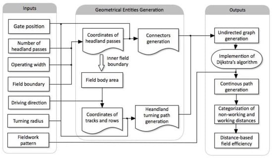
Figure 1. The graphical description of the developed tool.

The presented methodology, in its current form, considers the following assumptions-limitations:

(a)

Path generation for fields with obstacles is not considered.

(b)

The methodology can only be applied to non-capacitated field operations such as tillage, plough, and so on.

2.2. Generation of Continuous Path

2.2.1. Fixed Entities

Headland passes, field-work tracks, and rows, are referred to as fixed entities (Figure 2). These fixed entities are explained as follows:

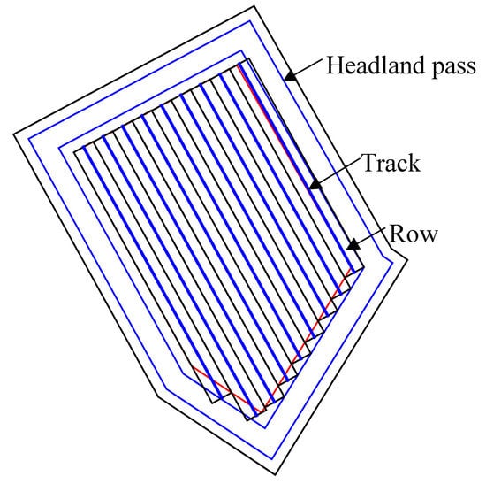
Figure 2. Illustrative example of fixed entities.

(a)

Headland pass (H): A headland pass is a concentric path covering the headland area at the same width as the operating width $\mathrm{w}$, of the implement which is made up of a set of sequentially clockwise ordered points. An inner boundary between the headland area and the work area is created at a distance half of the operating width w/2 from the last headland passes, the area enclosed by the inner boundary is denoted the field body area.

(b)

Row (R): The field body area is covered by parallel rows that transect the area. The width of each row equals the operating width w of the machine.

(c)

Field-work track (T): A track is represented by two ending points is the central line of a row and is used as the guidance line for the machine to cover each row.

2.2.2. Generation of Connectors

Connectors (as shown in Figure 3) are curved paths that inter-connect the gate points, the tracks, and the headland passes. The connectors are generated both in clockwise and anti-clockwise directions. The different types of connectors are explained as follows:

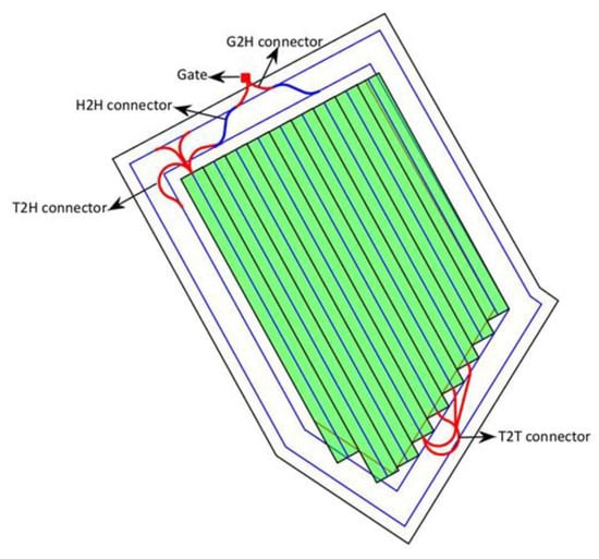
Figure 3. An illustrative example of four types of connectors.

• Gate-to-headland connector (G2H): A connection path between the field gate and the first headland pass. The G2H connectors provide the path for the agricultural vehicles to enter and exit the field area.
• Headland-to-headland connector (H2H): A connection path between two adjacent headland passes. These connectors are used for agricultural vehicles to move between headland passes.
• Track-to-headland connector (T2H): A connection path between a track end and a headland pass for agricultural vehicles to drive from a track to a headland pass or vice versa.
• Track-to-track connector (T2T): A connection path between a track end and another track end.

In the followings section, the procedure of generation of the aforementioned four types of connectors by using the Dubins curves path method [15] is described. A Dubins curve path is the shortest path between an initial point $(x_i,y_i$) with an initial heading $o_i$ and a goal point $(x_g,y_g$), with goal heading ${\mathsf{o}}_{\mathrm{g}}$ under the constraints of the bounded curvature not exceeding 1/r.

As the first step of generation of a G2H connector, the first headland pass is divided into segments by inserting points (red points in Figure 4a) between existing vertices based on a specified length ($l$), so that no segments are longer than this given threshold value. Additionally, a circle $C$ centred at gate E with radius t (t is set to $2*\mathrm{d}$, where d is the perpendicular distance of gate to the first headland pass) (Figure 4b) is created and only those headland pass points (black points in Figure 4c) within C are considered as an ending point of the G2H connector. Then, the shortest connection path (black curved path in Figure 4c) among all connection paths is generated (by implementing the Dubins method) between the gate, and the set of selected points within the circle C is selected as the G2H connector.

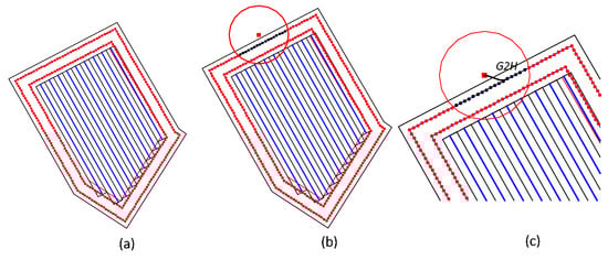
Figure 4. Illustration of procedures of generating gate to headland connector: (a) densify headland pass based on given length ($\mathrm{l}$); (b) generate a circle centered at gate $\mathrm{E}$ with radius $\mathrm{t}$; (c) generated $\mathrm{G}2\mathrm{H}$ connector.

To generate H2H and T2H connectors, the same procedure for generation of a connector G2H is implemented. The circle C is centred at the ending point of a G2H connector, and at the end of a track, for generation of a H2H and a T2H connector, respectively. Figure 5a,b illustrates the generated H2H and T2H connectors, respectively.

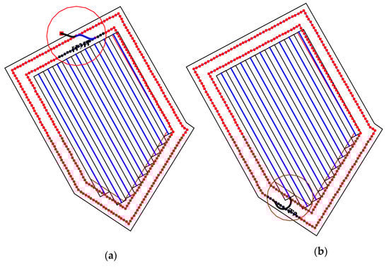
Figure 5. (a) The H2H connector (blue path), (b) the T2H connector (black path).

Regarding the generation of T2T connectors, only the connectors that are not crossing the field body area are generated. Figure 6 illustrates all the possible T2T connectors (red paths) from a track end to all other tracks’ ends inside the headland area.

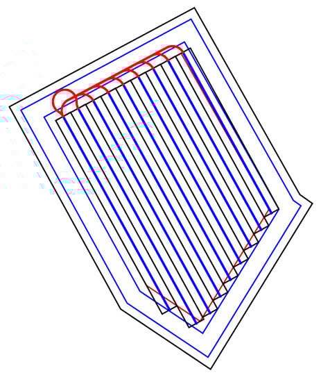
Figure 6. An illustrative example of track-to-track connectors (red curved paths) from one track end to all other tracks’ end.

2.2.3. Continuous Path Generation

With the above-mentioned fixed entities and connectors, a complete path can be generated to cover the entire field according to a specified fieldwork pattern (Figure 7a). Then, the problem of generation a path for field coverage is equivalent to the problem of traversing the undirected, weighted graph (Figure 7b) $\mathrm{G}=\left(\mathrm{V},\mathrm{E}\right)$, where $\mathrm{V}=\left\{{\mathrm{v}}_0,{\mathrm{v}}_1,\dots ,{\mathrm{v}}_{\mathrm{n},}\right\},\mathrm{n}\in \mathrm{Z}$, is the set of vertices consisting of all ending points of fixed entities and the connectors, with ${\mathrm{v}}_0$ representing the gate, and $\mathrm{E}=\left\{\mathrm{e}=\{{\mathrm{v}}_{\mathrm{i}},{\mathrm{v}}_{\mathrm{j}}\right\},\dots \},{\mathrm{v}}_{\mathrm{i}},{\mathrm{v}}_{\mathrm{j}}\in \mathrm{V}$, is the set of topological edges representing the fixed entities and connectors. Each edge $\mathrm{e}=\{{\mathrm{v}}_{\mathrm{i}},{\mathrm{v}}_{\mathrm{j}}\},\mathrm{i}\ne \mathrm{j}$ is characterized by its type $\mathrm{g}\in \left\{\mathrm{G}2\mathrm{H},\mathrm{H}2\mathrm{H},\mathrm{T}2\mathrm{H},\mathrm{T}2\mathrm{H},\mathrm{H},\mathrm{T}\right\}$, and its length that equals to the actual length of the corresponding edge of the fixed entities or connectors. In the undirected graph, all edges can be traversed from both directions in the form of sequence $\left[\mathrm{s},\mathrm{t}\right]$ when $\mathrm{m}=1$ or $\left[\mathrm{t},\mathrm{s}\right]$ when $\mathrm{m}=-1$.

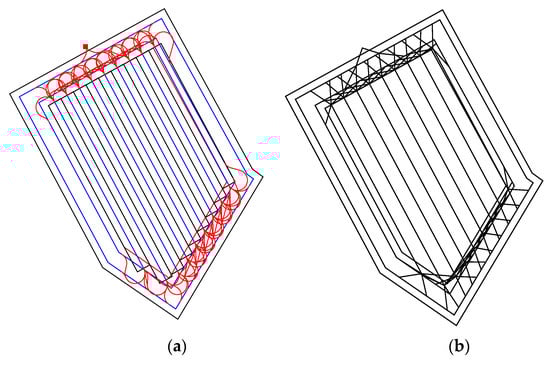
Figure 7. The fixed entities and all connectors (a), and their conversion to an undirected graph (b).

The entire continuous path for field coverage consists of four sub-paths, which are: the sub-path that connects the field gate with the outer headland pass, the headland passes traversing path (P_H) that connects all headland passes ${\mathrm{H}}_{\mathrm{i}=\left\{1,\dots ,\mathrm{h}\right\}}$ as one path that starts from the gate, the fieldwork tracks traversing path (P_T) that connects the ordered tracks and the field exiting path (P_B) for vehicle exiting field from the last track in $\mathsf{\rho }$ when the operation is done.

In order to generate these sub-paths, four methods are defined:

• $\mathrm{adj}\left({\mathrm{v}}_{\mathrm{i}},\mathrm{m}\right):$ is a function for headland traversing path ${\mathrm{P}}_{\mathrm{H}}$ generation, which finds all adjacent vertices {$\mathrm{v}$} of ${\mathrm{v}}_{\mathrm{i}}$ that directly link with ${\mathrm{v}}_{\mathrm{i}}$ in the graph based on the given direction $\mathrm{m}$.
• $\mathrm{seq}\left({\mathrm{v}}_{\mathrm{i}},{\mathrm{v}}_{\mathrm{j}}\right):$ finds the shortest path with a sequence of vertices from a source vertex ${\mathrm{v}}_{\mathrm{i}}$ to a target vertex ${\mathrm{v}}_{\mathrm{j}}$ on the graph (by implementing the Dijkstra’s algorithm [16].
• $\mathrm{get}\left(\mathrm{e},\mathrm{m}\right):$ returns the two vertex ids which correspond to edge $\mathrm{e}$ in sequence $\left[\mathrm{s},\mathrm{t}\right]$ when $\mathrm{m}=1$ or in sequence $\left[\mathrm{t},\mathrm{s}\right]$ when $\mathrm{m}=-1$.
• $\mathrm{find}\left({\mathrm{v}}_{\mathrm{i}},{\mathrm{v}}_{\mathrm{j}}\right):$ returns the edge $\mathrm{e}$ that links ${\mathrm{v}}_{\mathrm{i}}\mathrm{to},{\mathrm{v}}_{\mathrm{j}}$.
• $\mathsf{\Theta }\left(\mathrm{p}\right):$ returns the last vertex of path $\mathrm{p}$.

The procedures of generation are summarized in Algorithm 1, where the assumed headland traversing direction is clockwise $(m=1$).

Algorithm 1. Pseudo codes for continuous path generation.
Initialization:
Path$p$is initialized as set$p$=$\left\{v_0\right\}$that starts at gate.
${\mathit{P}}_{\mathit{H}}$path generation:
	Get all edges with type$H$,$se{t}_H =\left\{e_i\right\} where e_i·type ==H;$
	While$se{t}_H\ne \varnothing$
		Apply$adj\left(\Theta \left(p\right),1\right)\to \left\{v\right\}$ to get all adjacent vertices of the last vertex of path $p$;
		$If \forall x\in \left\{v\right\},e= find\left(\Theta \left(p\right),x\right) such that e\in se{t}_H and e·type ==H$;
		Then add e to path$p = p{\cup }^{\text{}}e$; and remove$e$from$se{t}_H: se{t}_H=se{t}_H\setminus e$;
		Else if$e·type ==H2H$,then add headland connector e to path$p = p{\cup }^{\text{}}e$.
	End
${\mathit{P}}_{\mathit{T}}$path generation:
	$p_{temp}= get\left(e_1,d_{e_1}\right)$;
	$p=p{\cup }^{\text{}}seq\left(\Theta \left(p\right),\Theta \left(p_{temp}\right)\right)$# Find the path from last vertex of$p$to starting vertex of track edge$e_1$;
	For$i= 1:(n-1$) do:
	$p=p{\cup }^{\text{}}get(e_i,d_{e_i})$; # Add vertices of track edge$e_i$to path$p$
	$p=p{\cup }^{\text{}}seq\left(\Theta \left(p\right),e_{i+1}\right)$; # Add path that is from end vertex of$e_i$to start vertex of$e_{i+1}$to path$p$
	$p=p{\cup }^{\text{}}get(e_i,d_{e_{i+1}})$; # Add vertices of track edge$e_{i+1}$to path$p$
	End
$P_B$path generation:
	$p=p{\cup }^{\text{}}seq\left(\mathsf{\Theta }\left(p\right),v_0\right)$; # Exiting field from last vertex of path$p$

2.2.4. Distance-Based Field Efficiency

In order to quantify the performance of a machinery system (tractor-implement or self-propelled machine), the distanced-based field efficiency is defined, as a function of the field shape, the machinery features, the operating width, and the fieldwork pattern, $\mathrm{FTE}:\to \mathrm{FTE}\left(\mathrm{B},\mathrm{w},\mathrm{u},\mathrm{h},\mathrm{r},\mathrm{E},\mathrm{F}\right)$, and is expressed as:

$$\mathrm{FTE}=\frac{{\sum }_{\mathrm{i}=1}^{\mathrm{h}}\mathrm{d}\left({\mathrm{H}}_{\mathrm{i}}\right)++{\sum }_{\mathrm{i}=1}^{\mathrm{n}}\mathrm{d}\left({\mathrm{T}}_{\mathrm{i}}\right)}{\mathrm{d}\left(\mathrm{p}\right)}$$

(1)

where $\sum _{\mathrm{i}=1}^{\mathrm{h}}\mathrm{d}\left({\mathrm{H}}_{\mathrm{i}}\right)$, $\sum _{\mathrm{i}=1}^{\mathrm{n}}\mathrm{d}\left({\mathrm{T}}_{\mathrm{i}}\right)$ is the total effective length of headland passes and tracks, respectively, while $\mathrm{d}\left(\mathrm{p}\right)$ is the total length of the continues path.

2.3. Sample Fields Scenarios

In order to show the degree of the dependence of the field efficiency on the operational features, a number of scenarios have been defined. Specifically, a number of 864 scenarios were generated derived from the consideration of six field shapes, three conventional fieldwork patterns, four driving directions, and twelve combinations of turning radius and implement width. The specific selected values of input parameters were:

(a)

Field : Six different template fields (Figure 8) with the same field area (10 ha) were selected as test fields. These artificial field shapes have been used in a number of studies of agricultural machinery management [17,18,19,20].

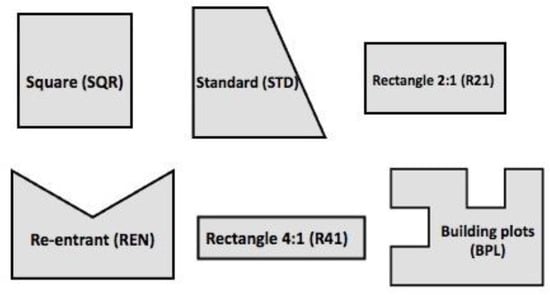Figure 8. The six template fields that were selected as test fields.

(b)

Machinery system: Three different types of machinery with different implements were considered in terms of sizes and maneuverability (minimum turning radius). Specifically, a large sized machine with a minimum turning radius of 6 m, a medium sized machine with a minimum turning radius of 4.5 m, and a small sized unit with minimum turning radius of 3 m, were selected. The selected implements’ width ranged from 3 m to 12 m. The specific test setups of machinery and implements (Table 1) have been selected as typical configurations implemented in field operation management assessments [17,18].

Table 1. Tested setups of machinery and implements.

$\mathbf{Minimum}\mathbf{Turning}\mathbf{Radius} \mathit{r}\left(\mathbf{m}\right)$		$\mathbf{Operating}\mathbf{Width}\mathit{w}\left(\mathbf{m}\right)$
Large size machine	6	4.5	7.5	9	10.5	12
Medium size machine	4.5	4.5	6	7.5	9	-
Small size machine	3	3	4.5	6	-	-

(c)

Fieldwork pattern: Three different common used fieldwork patterns (Figure 9a, AB; Figure 9b, SF; and Figure 9c, BL) were selected for the assessment. Each fieldwork pattern is represented mathematically with the traversal function, which produces the traversal sequence of the field tracks. The specific traversal functions of these three patterns are provided in Bochtis et al. (2013) [17]. The fieldwork pattern defines the traversal sequence of field-work tracks, thereby determining the total non-working turning distance in the headland area, and subsequently determining how efficient the machinery performs, in terms of distance covered [21].

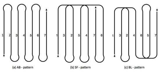Figure 9. Three conventional fieldwork patterns, (a) AB—pattern, (b) SF—pattern and (c) BL—pattern used in the tests.

(d)

Driving direction: The driving direction is an important factor in determining the number of tracks and their length, and subsequently affecting the field efficiency. Four driving directions ($\mathsf{\theta }$ = $0°$, $30°$, $60°$, and $90°$) were selected.

3. Results

3.1. Effect of Field Shape on FTE

Figure 10 provides the average, minimum, and maximum FTE values for all tested scenarios in each template field shape (Figure 8). The specific scenarios for which the FTE receives the minimum and maximum values in each individual field template, are given in Table 2. Significant variations in the average value of FTE were found between these six fields. As expected, odd shapes, such as REN, BPL are characterized by lower average values of FTE when compared to more regular shapes, i.e., SQR, STD, R21 and R41. The same findings are derived by other studies [7,22]. The FTE also varied significantly in the same field shape when using different setups of test parameters. The discrepancy between the minimum and maximum FTE in the same field shape is between 15% (in the case of SQR field) and 23%. (in the case of the BPL field).

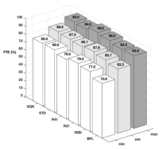
Figure 10. The minimum (min), average (ave), and maximum (max) field traversing efficiency (FTE) for each template field.

Table 2. The scenarios for min, max computed FTE in each test field.

Field Shape	Scenario Returning Minimum FTE				Scenario Returning Maximum FTE
	Pattern	Width (m)	Radius (m)	Direction (Degrees)	Pattern	Width (m)	Radius (m)	Direction (Degrees)
SQR	SF	12	6	30	BL	4.5	3	0
STD	SF	12	6	30	BL	3	3	0
R41	AB	4.5	6	30	AB	6	3	90
R21	SF	12	6	30	AB	4.5	3	90
REN	SF	12	6	30	BL	3	3	0
BPL	SF	9	6	60	AB	6	3	0

3.2. Effect of Fieldwork Pattern on FTE

It can be seen from Figure 11 that the AB and BL patterns are superior to the SF one, when comparing the resulting average FTE for each one of the individual sample fields. Therefore, selection of a suitable fieldwork pattern for a particular field can improve the machinery performance substantially. For instance, in the BPL field, the average FTE for the SF pattern is 7.6% higher than its counterpart for the AB pattern. This fact has been already shown in a number of studies.

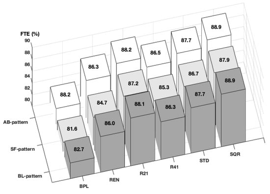
Figure 11. Average FTE for the three selected fieldwork patterns (AB, SF, and BL) in all template field shapes.

3.3. Effect of Driving Direction on FTE

As it is shown in Figure 12 the driving direction of 90° yielded the higher average FTE than the other tested directions. Even in the same type of field, the FTE also varied substantially when using different directions. For instance, the discrepancy of the average FTE is up to about 10% when comparing the applied driving direction $0°$ and $90°$ in R41 field. More tracks require more turns to cover the same field area, and subsequently resulting in lower field efficiency. Taking R41 as an example, the driving direction $0°$ produces 158 more tracks than using driving direction 90° when the operating width is 3 m.

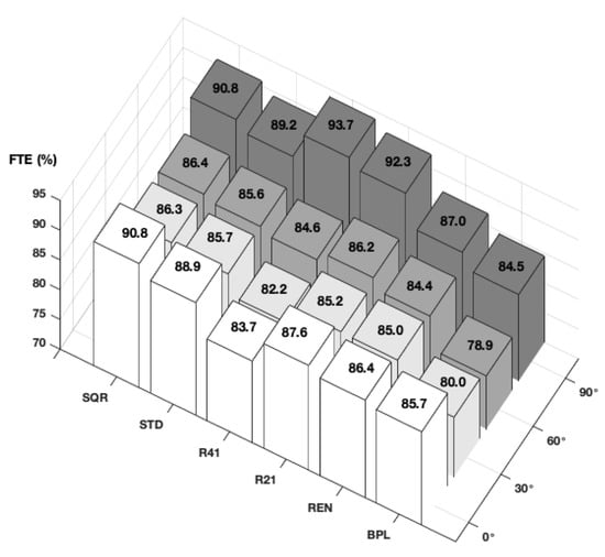
Figure 12. Average FTE for all template field shapes in each driving direction.

4. Discussion and Conclusions

In this paper, a new index for the efficiency of field operations was presented. This new index, FTE, provides an objective measure for the operational productivity since it is a function of well-defined and measurable features, including the field area and shape (field features), the machines’ operating width and turning radius (machinery features), the driving direction and the field-work pattern (operating features).

A number of scenarios, in terms of the above-mentioned features interaction, have been generated in order to demonstrate the sensitivity of the FTE to that features. The values of the FTE ranged between 70% and 98% for all tested scenarios. It is worth noting that the selection of the machinery features to be tested, provides a representative range in terms of operating width of the implements (4.5 m to 12 m) and the tractors’ size (minimum turning radius between 3 m and 6 m), and field-work patterns selected regard the most common patterns in agricultural field area coverage. An average value of the FTE has been also calculated based on the mix of all (realistic) combinations between the machinery and operating features for a specific field. To this end, this average can provide an index for a specific field that represents its operability as a function solely of its shape and total area. However, generating a field operability index is an issue of further research, since a more comprehensive and well-defined group of alternatives have to be generated to provide this average value. These alternatives include, as an example, the exhaustive enumeration of all feasible driving directions (and not just the use of the indicative directions of $0°$, $30°$, $60°$, and $90°$ in the case of artificial fields and the two perpendicular directions, namely the parallel and the vertical to the longest field edge, in the case of real fields.

The total longest productive travel length depends on the operating width (shorter operating width results to higher productive travelled distance) and for the same operating width depends on the area overlaps which are a function (given a fixed operating width) of the travelling direction. For the cases presented in Table 2, it is clear that for the cases of SQR, STD, R21, REN, and BPL the maximum FTE corresponds to longest travelled productive distances, while in the case of R41 the diversion between the min and max FTE values is attributed to the driving direction.

The method can be easily implemented in real fields. As an example, Figure 13 shows the generated continuous paths with corresponding FTE for two fields implementing three different field-work patterns.

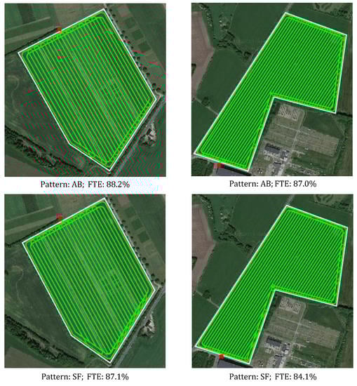
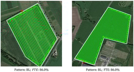
Figure 13. Demonstration of the effect of the field-work pattern on FTE. Other parameters are the same for all cases (operating width: 9 m; turning radius: 6 m; number of headlands: 2).

The approach can also be implemented also as decision support system for the field operational planning since the process of selecting the optimal combination of features such as operating width, driving direction, and field-work pattern it is not a trivial one. As for example, Figure 14 depicts a field implementation showing the variability of FTE in different operational setups for this field. It can be seen that by comparing the FTE between the configurations in Figure 14a,b, the one with the narrower operating width (b) results to a higher FTE compared with the larger width (a) due to the selection of the SF pattern in the former case. Analogously, by comparing the FTE configurations between Figure 14c,d, the shorter operating width results to a higher FTE due to the selection of another field-work pattern. Zhou et al., (2015) was shown that the improvement in the field efficiency can be up to 7% by adopting an appropriate fieldwork pattern [23].

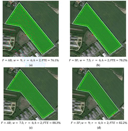
Figure 14. Demonstration of generated continuous paths with FTE on two selected fields (F: pattern; w: width; r: radius; h: headlands).

This first approach on FTE definition and estimation process presents a number of limitations. Specifically, these limitations include the path generation in fields with obstacles, in fields with un-even terrain, and in capacitated operations. Although there are existing methods for the generation of such paths (e.g., field with obstacles: [24,25], three-dimensional path planning: [26,27], capacitated operations [28,29]), there are optimization processes involved meaning that the generated paths can be also near-optimal solutions and thus biasing the objectiveness of the estimation of the field efficiency. In other words, the value of the estimated FTE will depend on the methodology followed. The inclusion of methods that generates these paths in the FTE estimation process and the necessary introduction of optimality conditions is an issue of further research.

References

- Hunt, D. Farm Power and Machinery Management; IOWA University Press: Iowa City, IA, USA, 2001; Volume I, pp. 77–93. [Google Scholar]
- Bochtis, D.D.; Sørensen, C.G.; Busato, P.; Hameed, I.A.; Rodias, E.; Green, O.; Papadakis, G. Tramline establishment in controlled traffic farming based on operational machinery cost. Biosyst. Eng. 2010, 107, 221–231. [Google Scholar] [CrossRef]
- Lampridi, M.G.; Kateris, D.; Vasileiadis, G.; Marinoudi, V.; Pearson, S.; Sørensen, C.G.; Balafoutis, A.; Bochtis, D. A Case-Based Economic Assessment of Robotics Employment in Precision Arable Farming. Agronomy 2019, 9, 175. [Google Scholar] [CrossRef]
- Busato, P.; Berruto, R.; Saunders, C. Logistics and efficiency of grain harvest and transport systems in a south australian context. In American Society of Agricultural and Biological Engineers Annual International Meeting 2008, ASABE 2008; American Society of Agricultural and Biological Engineers: St. Joseph, MI, USA, 2008; Volume 9, pp. 5336–5347. [Google Scholar]
- Li, Y.L.; Yi, S.P. Improving the efficiency of spatially selective operations for agricultural robotics in cropping field. Span. J. Agric. Res. 2013, 11, 56–63. [Google Scholar] [CrossRef]
- Grisso, R.D.; Kocher, M.F.; Adamchuk, V.I.; Jasa, P.J.; Schroeder, M.A. Field efficiency determination using traffic pattern indices. Appl. Eng. Agric. 2004, 20, 563–572. [Google Scholar] [CrossRef]
- Oksanen, T. Shape-describing indices for agricultural field plots and their relationship to operational efficiency. Comput. Electron. Agric. 2013, 98, 252–259. [Google Scholar] [CrossRef]
- Vizzari, M.; Santaga, F.; Benincasa, P. Sentinel 2-Based Nitrogen VRT Fertilization in Wheat: Comparison between Traditional and Simple Precision Practices. Agronomy 2019, 9, 278. [Google Scholar] [CrossRef]
- Scudiero, E.; Teatini, P.; Manoli, G.; Braga, F.; Skaggs, T.; Morari, F. Workflow to Establish Time-Specific Zones in Precision Agriculture by Spatiotemporal Integration of Plant and Soil Sensing Data. Agronomy 2018, 8, 253. [Google Scholar] [CrossRef]
- Bochtis, D.D.; Sørensen, C.G.; Jørgensen, R.N.; Green, O. Modelling of material handling operations using controlled traffic. Biosyst. Eng. 2009, 103, 397–408. [Google Scholar] [CrossRef][Green Version]
- Skou-Nielsen, N.; Villa-Henriksen, A.; Green, O.; Edwards, G.T.C. Creating a statistically representative set of Danish agricultural field shapes to robustly test route planning algorithms. Adv. Anim. Biosci. 2017, 8, 615–619. [Google Scholar] [CrossRef]
- Zandonadi, R.S.; Luck, J.D.; Stombaugh, T.S.; Shearer, S.A. Evaluating field shape descriptors for estimating off-target application area in agricultural fields. Comput. Electron. Agric. 2013, 96, 217–226. [Google Scholar] [CrossRef]
- Larson, J.A.; Velandia, M.M.; Buschermohle, M.J.; Westlund, S.M. Effect of field geometry on profitability of automatic section control for chemical application equipment. Precis. Agric. 2016, 17, 18–35. [Google Scholar] [CrossRef]
- Martelloni, L.; Fontanelli, M.; Pieri, S.; Frasconi, C.; Caturegli, L.; Gaetani, M.; Grossi, N.; Magni, S.; Pirchio, M.; Raffaelli, M.; et al. Assessment of the Cutting Performance of a Robot Mower Using Custom Built Software. Agronomy 2019, 9, 230. [Google Scholar] [CrossRef]
- Dubins, L.E. On Curves of Minimal Length with a Constraint on Average Curvature, and with Prescribed Initial and Terminal Positions and Tangents. Am. J. Math. 1957, 79, 497–516. [Google Scholar] [CrossRef]
- Chen, J. Dijkstra’s shortest path algorithm. J. Formaliz. Math. 2003, 15, 237–247. [Google Scholar]
- Bochtis, D.D.; Sørensen, C.G.; Busato, P.; Berruto, R. Benefits from optimal route planning based on B-patterns. Biosyst. Eng. 2013, 115, 389–395. [Google Scholar] [CrossRef]
- Rodias, E.; Berruto, R.; Busato, P.; Bochtis, D.; Sørensen, C.; Zhou, K. Energy Savings from Optimised In-Field Route Planning for Agricultural Machinery. Sustainability 2017, 9, 1956. [Google Scholar] [CrossRef]
- Gunnarsson, C.; Vågström, L.; Hansson, P.A. Logistics for forage harvest to biogas production-Timeliness, capacities and costs in a Swedish case study. Biomass Bioenergy 2008, 32, 1263–1273. [Google Scholar] [CrossRef]
- Witney, B. Choosing & Using Farm Machines; Longman Higher Education: Essex, UK, 1988. [Google Scholar]
- Bochtis, D.; Griepentrog, H.W.; Vougioukas, S.; Busato, P.; Berruto, R.; Zhou, K. Route planning for orchard operations. Comput. Electron. Agric. 2015, 113, 51–60. [Google Scholar] [CrossRef]
- Zhou, K.; Leck Jensen, A.; Bochtis, D.D.; Sørensen, C.G. Simulation model for the sequential in-field machinery operations in a potato production system. Comput. Electron. Agric. 2015, 116, 173–186. [Google Scholar] [CrossRef]
- Zhou, K.; Jensen, A.L.; Bochtis, D.D.; Sørensen, C.G. Quantifying the benefits of alternative fieldwork patterns in a potato cultivation system. Comput. Electron. Agric. 2015, 119, 228–240. [Google Scholar] [CrossRef]
- Zhou, K.; Leck Jensen, A.; Sørensen, C.G.; Busato, P.; Bothtis, D.D. Agricultural operations planning in fields with multiple obstacle areas. Comput. Electron. Agric. 2014, 109, 12–22. [Google Scholar] [CrossRef]
- Boryga, M.; Graboś, A.; Kołodziej, P.; Gołacki, K.; Stropek, Z. Trajectory Planning with Obstacles on the Example of Tomato Harvest. Agric. Agric. Sci. Procedia 2015, 7, 27–34. [Google Scholar] [CrossRef]
- Hameed, I.A.; Bochtis, D.D.; Sørensen, C.G.; Jensen, A.L.; Larsen, R. Optimized driving direction based on a three-dimensional field representation. Comput. Electron. Agric. 2013, 91, 145–153. [Google Scholar] [CrossRef]
- Hameed, I.A.; la Cour-Harbo, A.; Osen, O.L. Side-to-side 3D coverage path planning approach for agricultural robots to minimize skip/overlap areas between swaths. Robot. Auton. Syst. 2016, 76, 36–45. [Google Scholar] [CrossRef]
- Hameed, I.A.; Bochtis, D.D.; Sørensen, C.G.; Vougioukas, S. An object-oriented model for simulating agricultural in-field machinery activities. Comput. Electron. Agric. 2012, 81, 24–32. [Google Scholar] [CrossRef]
- Jensen, M.F.; Bochtis, D.; Sørensen, C.G. Coverage planning for capacitated field operations, part II: Optimisation. Biosyst. Eng. 2015, 139, 149–164. [Google Scholar] [CrossRef]
© 2020 by the authors. Licensee MDPI, Basel, Switzerland. This article is an open access article distributed under the terms and conditions of the Creative Commons Attribution (CC BY) license (http://creativecommons.org/licenses/by/4.0/).