3.1. Simulated Model
For the actual blade vibration measurement, even if the blade dynamic behavior is fully understood, it is still difficult to eliminate uncertainties in the measurement data [
33,
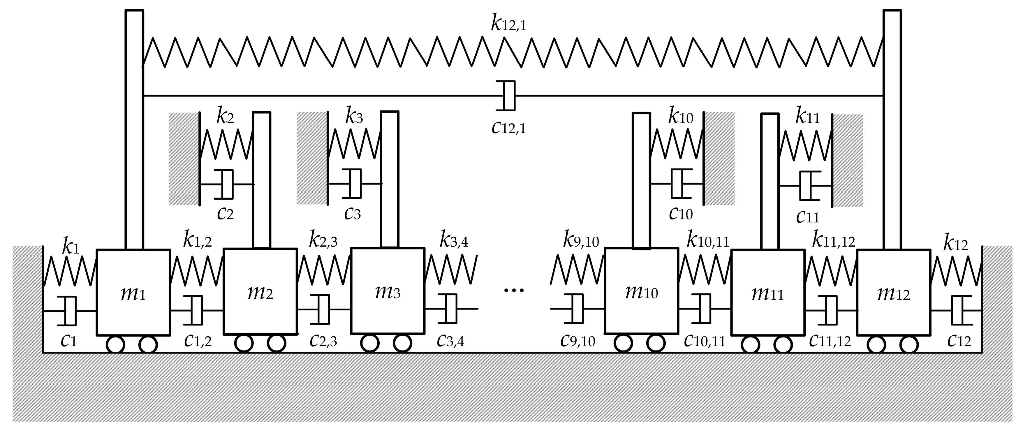
34], such as speed fluctuations, system random errors, etc. These uncertainties will affect the evaluation accuracy, therefore, it is better to use simulated data without measurement uncertainties to evaluate the accuracy of the reconstruction methods. A 12-blade assembly simulator was used to evaluate the ICFF performance. The schematic of the simulated model was shown in
Figure 3. A mass-spring-damper system represents each blade, which is coupled to its two neighbors through two further spring–damper assemblies. A mathematical model was employed to simulate the forced vibration of the rotating bladed assembly. This mathematical model ignored the effects of the centrifugal force and temperature on the blade stiffness.
The mathematical model of the bladed assembly is given by:
where
M,
C,
K, and
F(
t) represent the mass matrix, damping matrix, stiffness matrix, and excitation force vector, respectively. Let
W(
i,
j) (1 ≤
i ≤ 12 and 1 ≤
j ≤ 12) represents the element at the
ith row and
jth column of the matrix
W, and above matrixes can be expressed as:
In Equation (14), use 1 for subscripts greater than 12 and 12 for subscripts less than 1. The excitation force
fi (t) on blade
i is given by:
where
Fi is the amplitude of the excitation force, and
N represents the count of the blade.
N was set to 12 in this paper.
The quality of probe distribution is represented by the probe spacing on the resonance (PSR). The PSR is the ratio of the difference between the times of arrival of a blade at the first and last probe to the period of the blade response at resonance [
35], i.e.,:
where
ωn represents the natural angular frequency.
Further details on the mathematics of the simulator are given by the literature [
36]. According to the literature [
37,
38], the mistuning coefficient Δ
fi and the coupling coefficient
hi are defined to characterize the degree of blade mistuning and the coupling between blades. The concrete expressions of these two parameters are:
where the subscripts
i and
j represent the blade number, and
k represents the blade nominal stiffness. Let the nominal mass
m, stiffness
k, and damping
c be 1 kg, 8.1 × 10
5 N/m, and 9 N∙s/m, respectively. Then, the nominal natural frequency of the blade is 900 rad/s according to Equation (18):
Let the distribution of the mistuning coefficients Δ
fi of the 12-blade assembly simulator conform to a Gaussian distribution with a mean of 0 and a standard deviation of 0.04. The distribution of Δ
fi is shown in
Table 1. Assume that the blade actual mass
mi (
i = 1, 2, 3… 12) is equal to nominal mass
m. The actual natural frequency of the blade was calculated according to Equations (17)–(18) and
Table 1, which is shown in
Figure 4.
3.2. Simulated Test
The object of the simulated test was to assess analysis techniques for determining the EO and amplitude. Several exhaustive tests were performed using BTT data obtained from the simulator to evaluate the accuracy of the reconstruction method and their sensitivity to various test parameters. These parameters were:
- (1)
Probe spacing on the resonance (PSR);
- (2)
The number of revolution (n);
- (3)
Engine order (EO);
- (4)
Inter-blade coupling of the mistuned blade (ICoMB);
- (5)
The number of probes (g);
- (6)
Noise-to-signal ratio (NSR).
The NSR is defined as the ratio of the r.m.s. value of the noise to the value of the ‘clean’ amplitude of the blade. The NSR was set to 100 points averagely distributed in the range from 0.01 to 0.3. For the same NSR, a white noise generator was used to create 100 distinct noise sequences with which to corrupt the data obtained from the simulator. Each test was repeated using all the white noise sequences for each method on each NSR value. When there is noise in the data, the reconstruction method will contain two types of error [
39]:
- (1)
Bias is where the estimates are incorrect. It is caused by a summated squared noise term in the BTB matrix that does not tend to zero but increases with increasing noise levels. This is an effect of the ICFF model that is used.
- (2)
Scatter, where there is a range of estimates spread about the mean value, is caused by random variations in the data.
The mean and variance of the recovered EO and amplitude were computed, from which 95 percent confidence intervals were obtained. The best method will exhibit the lowest bias and, preferably, lowest scatter. Six test cases were designed to analyze and compare the performance of the TCFF and ICFF under different test conditions. These are shown in
Table 2. Test 1 was specifically chosen to be a very difficult case to analyze. Hence, the other tests were used to investigate whether specific changes in the parameters improve or degrade the performance of the method.
The PSR is a key factor that affects the performance of all BTT algorithms. It is also commonly used to determine the quality of probe distribution for blade synchronous vibration measurement. Currently, there are corresponding methods for optimizing the probe installation layout [
40]. Combined with the FEM, the optimization of probe layout can be achieved in actual engineering measurement. Therefore, we set the PSR to a high value (98%) in Test 1. In engineering applications, the probe is inevitably affected by the temperature, airflow, etc., and in severe cases, the measurement data will not be available. In this case, where a limited number of probes were used to measure blade vibration, the failed probe could not participate in the blade vibration analysis, which destroyed the optimization of the probe layout and resulted in a decrease of the PSR. For this reason, the PSR was set to a low value (55 percent) in Test 2.
For TCFF, the blade vibration parameters can be calculated based on the single-revolution data obtained by multiple probes (usually four). However, it is impractical that the single-revolution data are used to identify the blade vibration parameters in engineering applications, considering the effects of system measurement errors. Just as the AR method does [
39], it is reasonable to select multi-revolution data, including the blade synchronous resonance region, to determine the true vibration parameters based on the average of the calculation results. For any curve fitting algorithm, such as the single-parameter method, the amount of selected data should include the complete blade resonance response region as much as possible, although there are no specific rules on how many data points should be selected. In the simulated tests, 30 (Test 1) and 50 (Test 3) data points were selected for identifying the vibration parameters to demonstrate the effects of the data amounts on the quality of the identification of each method.
BTT technology is sensitive to a mode with a large amplitude at the blade tip, such as the first-order bending mode. In actual rotating machinery operation, due to mechanical structure or airflow disturbance, the same vibration mode of the blade may be excited at different resonance rotating speeds corresponding to different EO. For BTT algorithms, analysis of the blade vibration at different resonance rotating speeds is essentially a process of reconstructing signals with different degrees of under-sampling. The EO (Test 1: EO = 10; Test 4: EO = 13) was used to analyze and compare the sensitivity of TCFF and ICFF to different degrees of under-sampling, and the EO was also an important parameter for the blade vibration analysis.
Based on the CFF theory, at least three probes are needed to monitor blade synchronous vibration. The least-square method is used to calculate the blade synchronous vibration parameters if more than three probes are used. The TCFF usually uses four probes to increase robustness. However, Tao OuYang used seven probes in the experimental verification of TCFF [
31]. So far, there is no optimal choice for the number of probes. Test 5 was designed to verify the performance of TCFF and ICFF on the different number of probes.
Mistuning is a universal feature of the objective existence of the blades, and if inter-blade coupling of the mistuned blade exists, it will affect the performance of the BTT algorithms that only analyze single-frequency signals, such as the single-parameter method, the two-parameter plot method, CFF, and TCFF. The same applies to the ICFF method proposed in this paper. Therefore, Test 6 was specially designed to analyze and compare the sensitivity of TCFF and ICFF to ICoMB.
The noise in the measurement data is difficult to eliminate. The “clean” simulated data was polluted by noise in all simulated tests to make the data closer to the real measurements. The anti-noise performance of each method was verified by using simulated data of different pollution degrees that were represented by the NSR value.
The monitor positions of the probes in Test 1, Test 3, and Test 6 were 0°, 13.1°, 25.3°, and 35.3°. The monitor positions of the probes in Test 4 were 0°, 11.3°, 13.3°, and 25.3°. In Test 2, the monitor positions of the probes were 0°, 6.3°, 10.1°, and 19.8°. In Test 5, the monitor positions of the probes were 0°, 6.3°, 13.1°, 19.1°, 25.3°, 30.2°, and 35.3°. The PSR in
Table 2 was calculated according to Equation (16). If the option of the ICoMB is “NO”, it means that the coupling coefficient is set to zero; if it is “Yes”, it means the coupling coefficient is set to nonzero. In this paper, the coupling coefficient
hi (
i = 1, 2, 3…, 12) was set to 0.1 for the option “Yes”. It is must be stressed that the blade vibration does not influence the adjacent blades when the coupling coefficient is set to zero, even under the condition that the blade is mistuned. For this, it is still a single-frequency vibration for the single blade. However, the synchronous resonance of the single blade will be a superposition of multiple-frequency vibration under the condition that the coupling coefficient is set to nonzero, and it is difficult to distinguish. The coupled vibration of the mistuned blade is a serious challenge for TCFF, since it assumes the blade response is of single-frequency vibration. According to the results shown in
Figure 4, the natural frequency of blade 7 is close to that of the adjacent blades. To evaluate the performance of ICFF under the condition of blade mistuning and inter-blade coupling, the simulated data of blade 7 were selected in the simulated tests. The rotating speed was set to accelerate uniformly from 300 to 2400 rpm, which included the resonance rotating speed for all simulated tests. Take the resonance rotating speed as the reference and select half
n points before and after the reference point to compose the number of revolutions
n. The results of each simulated test were analyzed as follows.
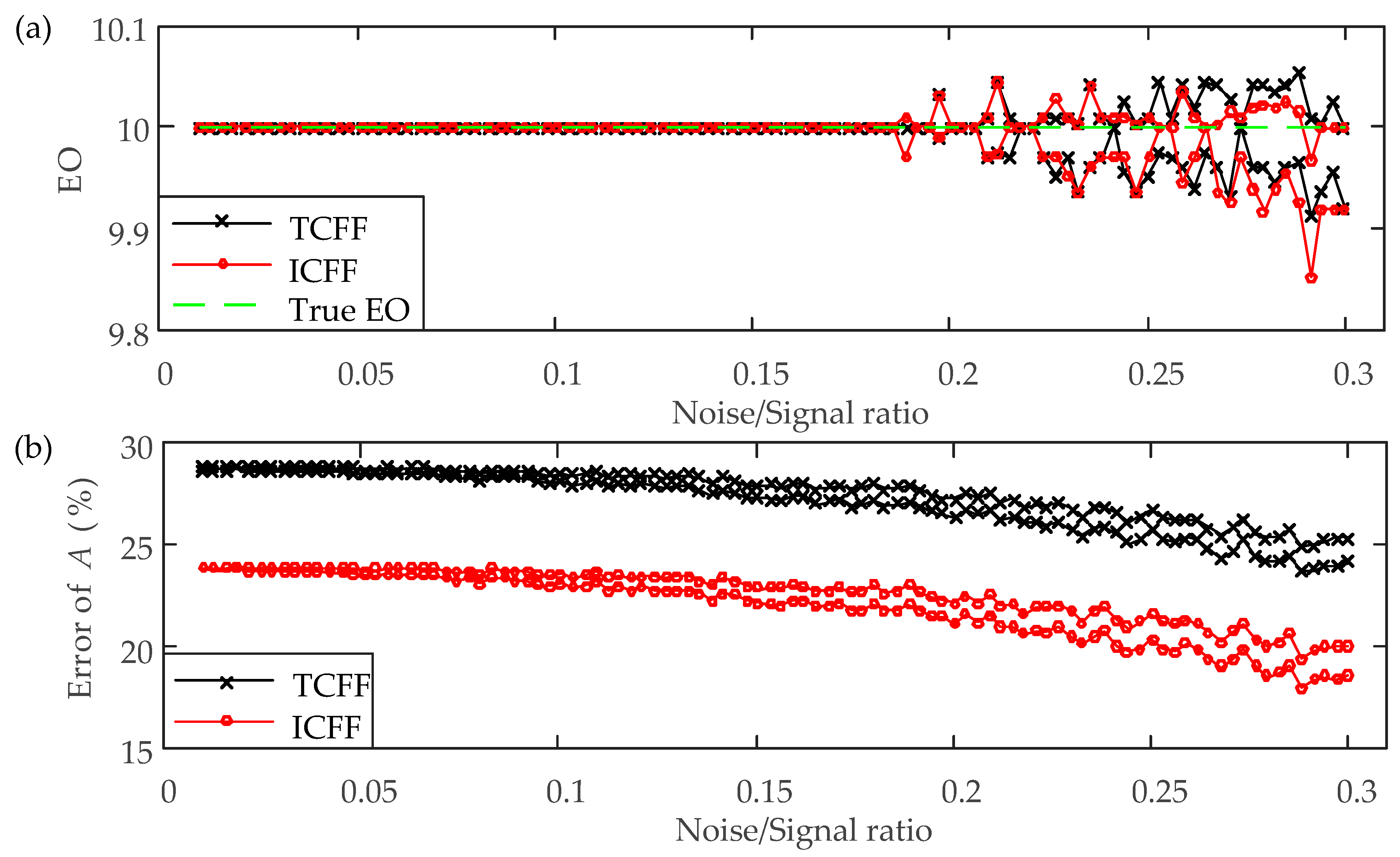
• Test 1:
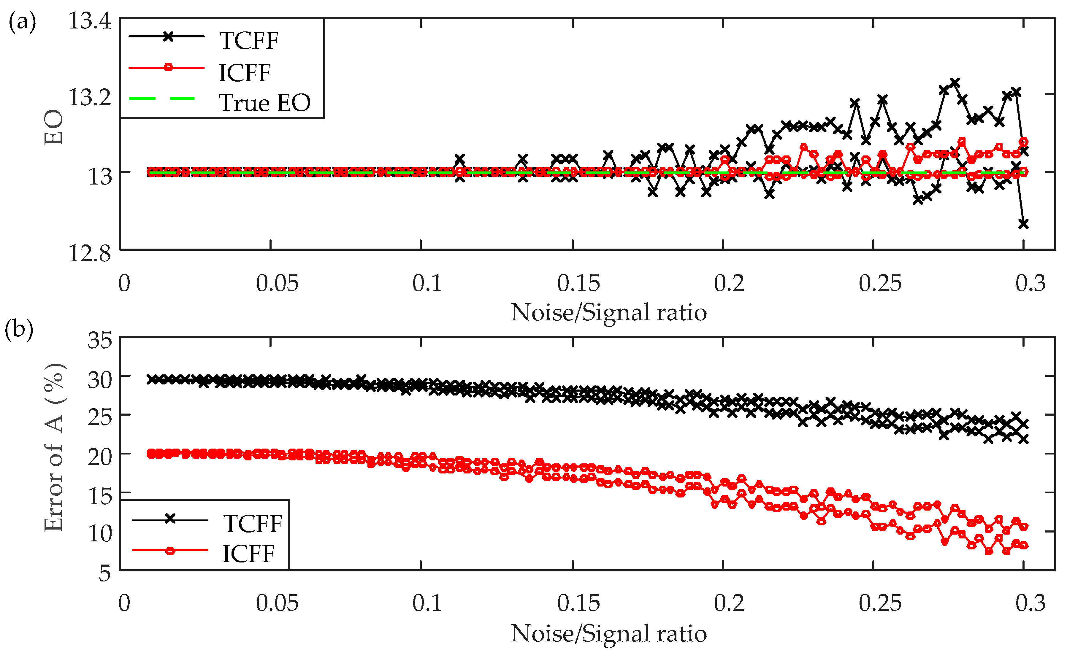
As expected, Test 1 was a very difficult case. As shown in
Figure 5a, the EO identification started to produce biased results at about NSR 0.16 for both methods. For tests with correct EO identification, the 95% confidence intervals of the relative error of the amplitude identification were calculated, which was shown in
Figure 5b. The intervals increased with the increase of the NSR for both methods. However, the relative error of amplitude identification of ICFF was lower than that of TCFF.
• Test 2:
Reducing the PSR value to 55 percent produced the most dramatic degrade in the quality of the identification. The correct EO identification did not occur for ICFF before NSR 0.15, and the deviation of EO identification was very large for both methods compared with Test 1. In order to compare the two methods synchronously,
Figure 6a only showed that the results of the EO identification in the NSR range of 0.15 and 0.30. The relative error of amplitude identification was calculated after NSR 0.15. The scatter of the relative error was higher than that of Test 1. As already discussed by other literature [
35,
36,
39], curve fits of lower PSR data are generally not conducive to parameter identification.
• Test 3:
Increasing the number of revolutions over which data were used for the identification process can improve the results. The results of EO identification started to be biased when the NSR increase to about 0.18 for both methods, which was shown in
Figure 7a. The NSR corresponding to unbiased identification was higher 0.03 than Test 1. However, relative error for amplitude identification increased with increasing the number of data, which was caused by a summated squared noise term in the
BTB matrix. This is an effect of the method model that is used. Although the relative error was increased for both methods, the ICFF error increased less than the TCFF.
• Test 4:
The results of Test 4 were shown in
Figure 8. Increasing the EO of the tip timing data had no visible effect on the accuracy of the EO identification for ICFF. However, the relative error of amplitude identification was higher than that of Test 1. For the same natural frequency, the larger EO, the higher degree of under-sampling. That means the number of samples was less for a period of vibration of the blade. The amplitude that recovered was more sensitive to the number of samples than the EO identification. Although the relative error was increased for both methods, the quality of ICFF was still higher than TCFF.
• Test 5:
Increasing the number of probes made the scatter of EO identification get larger for ICFF, which was shown in
Figure 9a. Meanwhile, the relative error of amplitude identification was increased for both methods, which was shown in
Figure 9b. The summated squared noise term in the
BTB matrix would increase with the number of probes. Then the squared noise term was transferred to amplitude identification.
Figure 9b still showed the relative error of ICFF was smaller than TCFF.
• Test 6:
The existence of the ICoMB did not have an effect on the EO identification for both methods, which was shown in
Figure 10a. BTT data that consists of two modes corresponding to different EO generally had negative effects on the quality of identification, especially for the reconstruction method that processes the single-frequency signals. However, it did not belong to the range considered in this paper. It needs some future work for processing the multi-frequency signals based on ICFF. The ICoMB made the quality of amplitude identification degrade, which was shown in
Figure 10b. However, the relative error of ICFF was still lower than that of TCFF.


