Article

Nonlinear Vibration Mitigation of a Beam Excited by Moving Load with Time-Delayed Velocity and Acceleration Feedback

1
School of Civil Engineering, Hunan University of Science and Technology, Xiangtan 411201, Hunan, China
2
Hunan Provincial Key Laboratory of Structures for Wind Resistance and Vibration Control, Hunan University of Science and Technology, Xiangtan 411201, Hunan, China
3
Department of Engineering Mechanics, State Key Laboratory of Structural Analysis for Industrial Equipment, Dalian University of Technology, Dalian 116023, China
*
Authors to whom correspondence should be addressed.
Appl. Sci. 2020, 10(11), 3685; https://doi.org/10.3390/app10113685
Submission received: 24 March 2020 / Revised: 29 April 2020 / Accepted: 21 May 2020 / Published: 26 May 2020
(This article belongs to the Section Acoustics and Vibrations)

Abstract

:
The time-delayed velocity and acceleration feedback control are provided to mitigate the resonances response of a nonlinear dynamic beam. By use of the method of multiple scales, the primary resonance and the 1/3 subharmonic resonance response of the controlled beam are analyzed. The excitation amplitude response peak and critical expression are obtained, and numerical simulations are also given. The effect of the feedback gains and time delayed on the steady-state response of the two types of resonances are investigated. The result show that time-delayed acceleration feedback control can effectively mitigate amplitude, and the main resonance response is affected periodically. Selecting reasonable control gain and time delay quantity can avoid the main resonance region and unstable multi-solutions, and can improve the efficiency of the vibration control.

1. Introduction

Beams are important structural components used in many practical engineering structures, such as gantry crane, etc. Under the dynamic loads of vehicles, wind, and earthquakes, the dynamic behaviors become more complicated [1,2,3]. As a very important topic in structural dynamics, the moving load problem of the beam is of practical importance in engineering. Kumar et al. [4] proposed a simple and compact formula to determine the free vibration responses of a uniform beam, which was applied to both lightly and heavily damped beams. Fiorillo and Ghosn [5] described a procedure to estimate the nonlinear ultimate load-carrying capacity of continuous beams by use of a combination of linear elastic influence lines for segments of the beam in appropriately selected damaged configurations.
Up to now, many studies have reported investigating vibration control of structures [6]. Lin et al. [7] studied the PTMD control on a benchmark tv tower under earthquake and wind load excitations. Sun et al. [8] investigated the exact H2 optimal solutions to inerter-based isolation systems for building structures. Besides, as a kind of active control, the time-delay feedback control technology has attracted wide attention because of its easy adjustment, wide application range, and high control efficiency. The robust control and the time delay control that could achieve good control performance of a dynamic beam structure system were presented [9,10]. Ji and Leung [11] studied the primary, superharmonic, and subharmonic resonances of a harmonically excited non-linear s.d.o.f. system with two distinct time-delays in the linear state feedback. Sadek et al. [12] studied feedback control with time-delay, which was employed to minimize the maximum deflection of a beam subjected to impulsive and/or short-time loads. Taffo and Siewe [13] investigated the dynamics of a parametrically excited quarter-car model with time delayed feedback position and linear velocity terms. Li et al. [14] studied the dynamics of a system of two Van der Pol oscillators with delayed position and velocity coupling by the method of averaging together with truncation of Taylor expansions. Hu et al. [15] presented analytical and numerical studies of the primary resonance and the 1/3 subharmonic resonance of a harmonically forced Duffing oscillator under state feedback control with a time delay. Wang and Hu [16] studied the stabilization of vibration systems via delayed state difference feedback. Maccari [17] investigated the primary resonance of a cantilever beam under state feedback control with a time delay. Zhao and Xu [18] applied the delayed feedback control to suppress the vibration of vertical displacement in a two-degree-of-freedom nonlinear system with external excitation. Alhazza et al. [19] investigated the non-linear vibrations of parametrically excited cantilever beams subjected to non-linear delayed-feedback control. More specifically, three non-linear cubic delayed-feedback control methodologies: position, velocity, and acceleration delayed feedback were examined. Peng et al. [20,21,22] studied the time delayed feedback control for beam structures. Lü et al. [23] investigated the local dynamics of an axially moving string under aerodynamic forces with a time-delayed velocity feedback controller.
In all the studies cited above, the linear and nonlinear dynamics were investigated. The primary resonance, super/subharmonic resonance and multi-frequency excitation resonance responses are all involved. These resonance forms are particularly important in flexible structures [24,25]. So the primary and 1/3 subharmonic resonance responses of a dynamics beam with moving load and time-delayed feedback is investigated in this study. Moreover, the vibration control equations we derived belong to duffing equations [26], which are delay differential equations with cubic nonlinearity.Despite the present work being focused on the dynamical response of a structural element, the amplitude equations describing its dynamics are also common to a wide variety of phenomena. They naturally appear in systems involving oscillations, ranging from population [27] and climate [28] cycles in the natural environment, the oscillatory nature of waves in fluids [29], or various applications in microelectromechanical systems (MEMS) [30,31], among others.
We organize the rest of this paper as follows. In Section 2, we introduce a nonlinear mathematical model of a dynamic beam subjected to moving load and time-delayed feedback. In Section 3 and Section 4, the resonance response of time-delayed velocity and acceleration feedback control are discussed by using the method of multiple scales, respectively. A discussion on comparing and a summary of results are presented in Section 5 and Section 6.

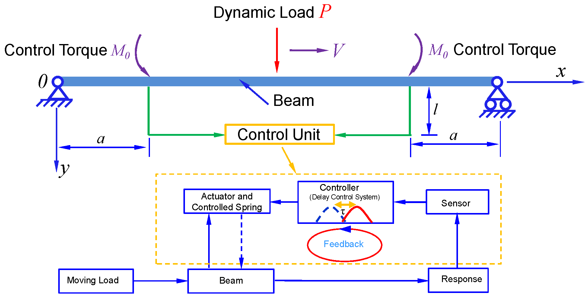
2. Controlled Beam Model and Equations of Motion

In this study, we consider a dynamic beam structure subjected to the dynamic load P, which moves along the longitudinal direction of the beam with a velocity V and under active control by a servomechanism, as shown in Figure 1. The motion equation of the beam is shown as follows [9]:
E I v + m v ¨ + c v ˙ = P δ ( x V t ) + M 0 δ ( x a ) M 0 δ ( x L + a ) ,
where the prime indicates the derivative with respecting to x and the dot indicates the derivative with respect to t; E is the Young’s modulus of the beam; I is the moment of inertia of the cross-section; v ( x , t ) is the transverse displacement of the beam; m is the mass per unit length of the beam; c is the damping coefficient; δ is the Dirac delta function and δ is the derivative; L is the span length of the beam; a is the distance between the servohinge and the end of the beam; In order to balance the bending deformation of the beam under moving load, a servomechanism is installed below the middle of the beam span to generate a control torque M 0 . The working principle is to adjust the control spring to achieve the control effect. The control torque is designated as:
M 0 = l K Δ = K l u ( t ) + l v ( a , t ) l v ( L a , t ) ,
where K is the stiffness of the spring; l is the arm length of servomechanism; u ( t ) is the spring displacement caused by servomechanism, and Δ is the displacement of the spring. When u ( t ) = 0 , it is a passive control system.
Using the Galerkin method, the equation of motion of the first mode can be written as (the details of the derivations are given in the Appendix A):
q ¨ ( t ) + ω 0 2 q ( t ) + μ q ˙ ( t ) = f sin ω t + α q 3 ( t ) + u ( t ) ,
where q ( t ) = ( 2 / L ) 0 L v ( x , t ) ϕ 1 ( x ) d x , ω 0 2 = ω 1 2 2 π K l cos π a L , μ = 2 ζ ω 1 , f = 2 P / ( m L ) , α = π 4 E 2 / ( L 4 A 2 ) , A is the cross-section area of the beam. u ( t ) is the active control force. In this paper, the time-delay speed feedback and time-delay acceleration feedback control strategies are adopted. Next, in Section 3 and Section 4, the primary resonance response and 1/3 subharmonic resonance response of the beam with the two different feedback controls are studied respectively.

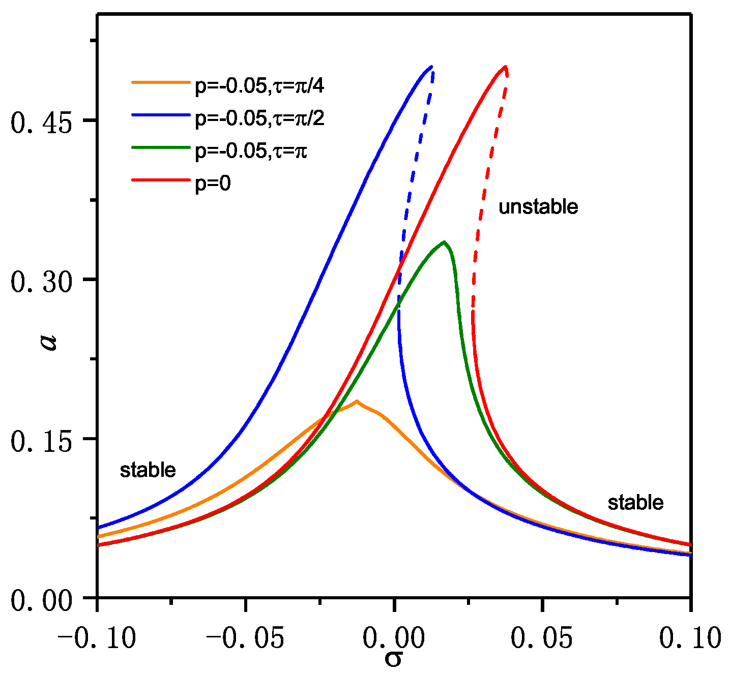
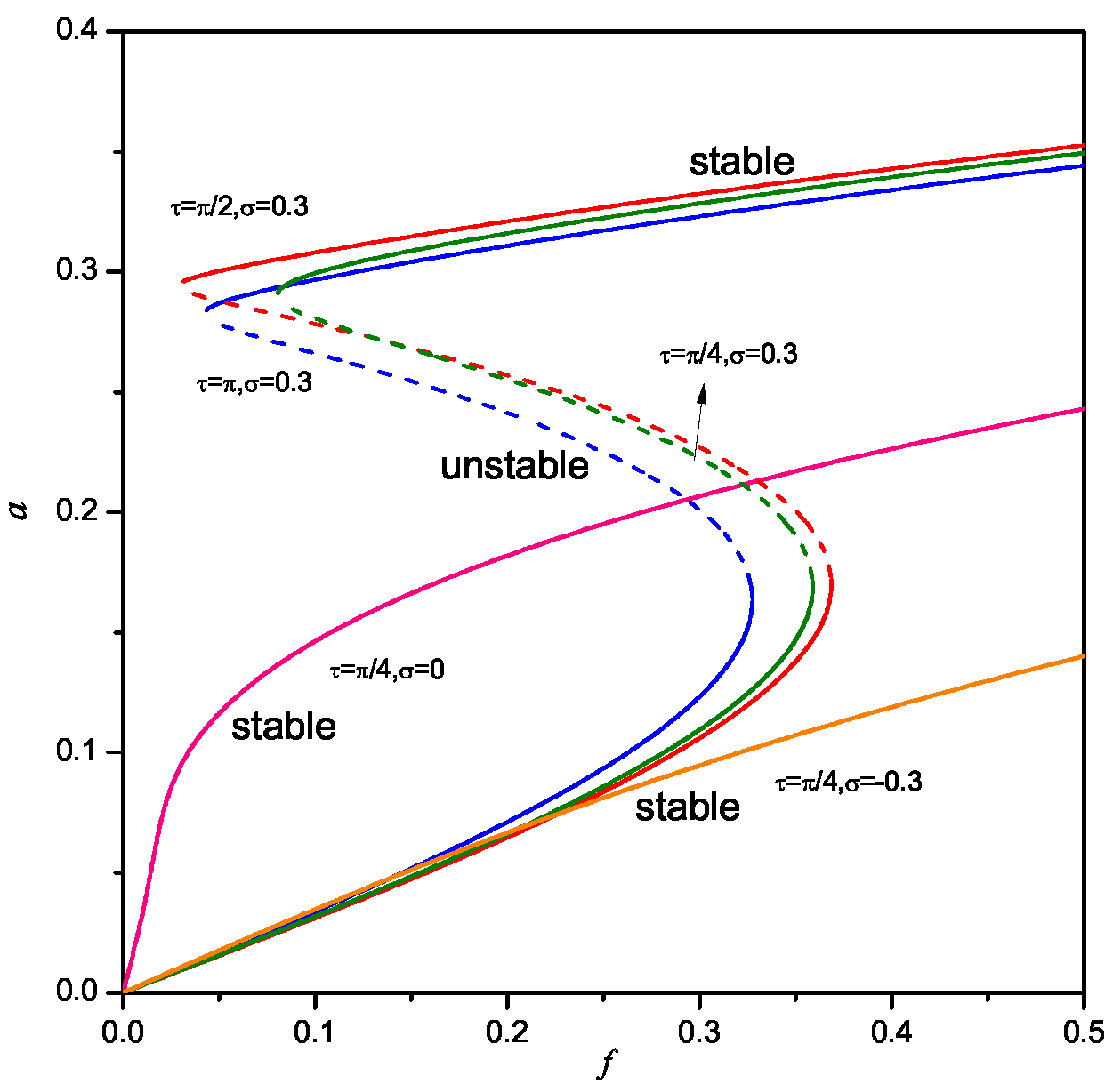
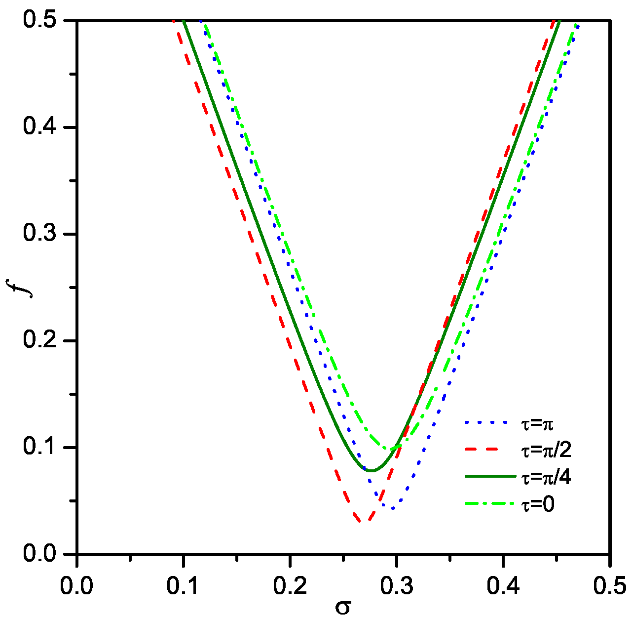
3. Time Delayed Velocity Feedback Control

In this section, the time delayed velocity feedback control strategy is adopted, i.e., u ( t ) = p q ˙ ( t τ ) , P is the control gain and τ is the time delay. Then using the method of multiple scales [26,32,33], the primary and 1/3 subharmonic resonances of the time delayed velocity feedback control are studied.

3.1. Nonlinear Primary Resonance Response

By using the method of multiple scales, the perturbation solution of Equation (3) is assumed as follows:
q = q 0 ( t 0 , t 1 ) + ε q 1 ( t 0 , t 1 ) + ,
where T 0 = t , T 1 = ε t . In the case of primary resonance, we let
ω = ω 0 + ε σ ,
where σ is the detuning parameter. Substituting Equations (4) and (5) into Equation (3) and equating coefficients of similar powers of ε yield the following equations:
D 0 2 q 0 + ω 0 2 q 0 = 0 .
D 0 2 q 1 + ω 0 2 q 1 = 2 D 0 D 1 q 0 μ D 0 q 0 + α q 0 3 + f sin ( ω 0 T 0 + σ T 1 ) + p D 0 q 0 ( t τ ) .
The solution of Equation (6) is written as follows:
q 0 = A ( T 1 ) e i ω T 0 + A ¯ ( T 1 ) e i ω T 0 .
Substituting Equation (8) into Equation (7) we obtain
D 0 2 q 1 + ω 0 2 q 1 = [ 2 i ω D 1 A i μ ω 0 A + 3 α A 2 A ¯ + f 2 e i σ T 1 + i ω p ( cos ω τ i sin ω τ ) A ] e i ω 0 T 0 + α A 3 e 3 i ω T 0 + c c ,
where c c denotes the conjugate term. Eliminating secular terms from Equation (9), we have
2 i ω 0 D 1 A i μ ω 0 A + 3 α A 2 A ¯ + f 2 e i σ T 1 + i ω 0 p ( cos ω τ i sin ω τ ) A = 0 .
Let A = 1 2 a exp ( i β ) and substituting it into Equation (10) and separating the real and imaginary part yield the averaged equation as follows:
a = μ a 2 f 2 ω sin γ + a p 2 cos ω 0 τ , a γ = σ a + 3 α a 3 8 ω 0 + f 2 ω cos γ a p 2 sin ω 0 τ ,
where γ = σ T 1 β . Then the frequency response relations are obtained by:
f 2 4 ω 0 2 = 1 4 ( μ p cos ω 0 τ ) 2 a 2 + [ ( σ p 2 sin ω 0 τ ) 3 α a 2 8 ω 0 ] 2 a 2 , tan γ = 4 ω 0 ( μ p cos ω 0 τ ) 8 ω 0 ( σ p 2 sin ω 0 τ ) + 3 α a 2 .
For a special case, the parameters μ , ω , α are confirmed as μ = 0.02 , ω = 1 , α = 0.4 . The frequency-response curves (a versus σ ) for the primary response are depicted in Figure 2. Selecting the control gain value p = 0.05 , it can be seen from the frequency amplitude curve that by adjusting different time delay, a better control effect can be obtained, and the peak value of the response can be significantly reduced. Figure 3 shows the variation of the response amplitude with the excitation amplitude for several values of σ and τ . These curves were obtained directly from Equation (12). We note that, depending on the value of σ , some curves are multivalued while others are single-valued.
It is seen that the saddle-node (SN) bifurcations located on the primary branch. Then, to determine the lowest excitation amplitude, the locus of the SN bifurcation points in the f σ plane is obtained in Figure 4 for p = 0.05 and different values of τ . It is shown that the minimum point determines the minimum excitation level below and the excitation frequency band can also be determined. As the time delay increases, the amplitude of the minimum excitation also decreases.
The trajectories of the damped motions of the nonlinear beam are plotted in Figure 5. Points P 1 and P 2 are stable foci, and point P 3 is a saddle point. All initial conditions in the shaded area lead to the steady-state solution on the lower branch P 1 , while all initial conditions in the unshaded area lead to the upper branch P 2 . Thus all the shaded area constitutes the domain of attraction of point P 1 , and all the unshaded area constitutes the domain of attraction of point P 2 .
Again, a small change in the initial conditions can produce large change in the response of the system: this is evidenced in Figure 6 by comparing the laws a ( t ) , γ ( t ) corresponding to conditions which just differ very little with regarding the amplitude.
The peak amplitude of the primary resonance, obtained from the first equation of Equations (12), is given by
a p = f 2 | u e | ω .
The critical force amplitude f c obtained from Equation (12) is
f c = 2 ω μ e 2 ω μ e / 3 α ,
for f < f c there is only one solution while for f > f c there are three.
Figure 7 corresponds to the critical force amplitude and the peak of the primary resonance changing with time delay τ . We must point out that the change rule of the critical force amplitude and the peak of the primary resonance are not wholly conformable. So the proper value of τ may take into account the requirement of engineering. By way of example, Figure 8 and Figure 9 shown the time history curves, phase diagram and frequency power spectrum of the primary resonance response are obtained numerically at time delay τ = π / 2 and τ = π , respectively.

3.2. 1/3 Subharmonic Resonance

To analyze subharmonic resonance for Equation (3), we introduce the detuning parameter σ according to
ω 0 = 1 3 ω + ε σ .
Substituting Equations (4) and (15) into Equation (3) and equating coefficients of like powers of e yields the following equations:
D 0 2 q 0 + 1 9 ω 2 q 0 = f sin ω T 0 ,
D 0 2 q 1 + 1 9 ω 2 q 1 = 2 D 0 D 1 q 0 2 3 ω σ q 0 μ D 0 q 0 + α q 0 3 + p D 0 q 0 ( t τ ) .
By solving Equation (16) for q 0 , we have
q 0 = A ( T 1 ) e i ω T 0 / 3 + 9 16 ω 2 F i e i ω T 0 + c c ,
where ’cc’ denotes the conjugate term. Substituting Equation (18) into Equation (17) yields
D 0 2 q 1 + 1 9 ω 2 q 1 = 2 3 D 1 i ω A 2 3 ω σ A i 3 μ ω A + 3 α A 2 A ¯ + 243 128 ω 2 α F 2 A + 27 16 ω 2 i α F A ¯ i 3 ω p cos 1 3 ω τ i sin 1 3 ω τ A e i ω T 0 / 3 + c c .
The secular term of Equation (19) vanishes if and only if
2 3 D 1 i ω A 2 3 ω σ A i 3 μ ω A + 3 α A 2 A ¯ + 243 128 ω 2 α F 2 A + 27 16 ω 2 i α F A ¯ i 3 ω p cos 1 3 ω τ i sin 1 3 ω τ A = 0 .
Letting A = a exp ( i φ ) into Equation (20) and separating the real part and the imaginary part, we obtain the autonomous differential equations governing the amplitude and the phase
a = 1 2 ( μ + p cos 1 3 ω τ ) a 81 32 α F a 2 cos ϕ , a ϕ = ( σ + p 2 ω sin 1 3 ω τ ) a + 729 256 ω α F a 9 α 2 ω a 3 81 32 α F a 2 sin ϕ ,
where ϕ ( T 1 ) = σ T 1 3 φ ( T 1 ) . From Equation (21), we get a set of algebraic equations that governs the amplitude a and the phase φ of the steady-state 1/3 subharmonic resonance
1 2 ( μ + p cos 1 3 ω τ ) a = 81 32 α F a 2 cos ϕ , ( σ + p 2 ω sin 1 3 ω τ ) a + 729 256 ω α F a 9 α 2 ω a 3 = 81 32 α F a 2 sin ϕ ,
whereby we have the frequency response relation between a and σ and that between φ and σ
1 4 μ e 2 a 2 + σ e 729 256 ω α F 2 9 α 2 ω a 2 2 a 2 ( 81 32 α F ) 2 a 4 = 0 , tan ϕ + 2 σ e + 729 α F / ( 256 ω ) 9 α a 2 / ω μ e = 0 ,
where
μ e = μ + p cos 1 3 ω τ , σ e = σ + p 2 ω sin 1 3 ω τ .
The first equation in Equations (23) shows that either a = 0 or
1 4 μ e 2 + σ e 729 256 ω α F 2 9 α 2 ω a 2 2 = ( 81 32 α F ) 2 a 2 ,
which is quadratic in a 2 . Its solution is
a 2 = ϱ ± ( ϱ 2 ι ) 1 / 2 ,
where
ϱ = 2 ω σ e 9 α 405 512 F 2 , ι = 2 ω 9 α 2 σ e 729 256 ω a F 2 2 + 1 4 μ e 2 .
We note that ι always positive, and thus nontrivial free-oscillation amplitudes occur only when ϱ > 0 and ϱ 2 ι , these conditions require that
F 2 < 1024 ω σ e 3645 α , α F 2 ω σ e 6561 α F 2 2048 ω 128 729 μ e 2 0 .
It follows from Equation (28) that, for given F and σ , nontrivial solutions can exist only if
ρ ( 4 ρ 2 6561 ) 1 / 2 ν ρ + ( 4 ρ 2 6561 ) 1 / 2 ,
where
ρ = σ e μ e , ν = 6561 α F 1024 ω μ e .
In the ( ρ , ν ) -plane the boundary of the region where nontrivial solutions can exist is given by
ν = ρ ± ( 4 ρ 2 6561 ) 1 / 2 ,
which is shown in Figure 10 for α > 0 . When these conditions hold, it is possible for the system to respond in such a way that the free-oscillation term does not decay to zero in spite of the presence of damping and in contrast with the linear solution. Moreover, in the steady-state, the nonlinearity adjusts the frequency of the free-oscillation term to one third the frequency of the excitation so that the response is periodic. Since the frequency of the free-oscillation term is one third that of the excitation, such resonances are called subharmonic resonances. Several frequency-response curves are shown in Figure 11.

4. Time Delayed Acceleration Feedback Control

In this section, we study the nonlinear response of the beam under time-delayed acceleration feedback, i.e., u ( t ) = p q ¨ ( t τ ) . Similar to the derivation process in Section 3, the frequency response equation of primary resonance response are obtained as follows:
f 2 4 ω 0 2 = 1 4 ( μ p ω 0 sin ω 0 τ ) 2 a 2 + [ ( σ + p ω 0 2 cos ω 0 τ ) 3 α a 2 8 ω 0 ] 2 a 2 , tan γ = 4 ω 0 ( μ p ω 0 sin ω 0 τ ) 8 ω 0 ( σ + p ω 0 2 cos ω 0 τ ) + 3 α a 2 .
The frequency-response curves of the first mode amplitude a as a function of the detuning parameter σ for the primary resonances response are shown in Figure 12. Compared with time-delayed velocity feedback, the same control parameters are selected here. As can be seen from the Figure 12, when the control gain is p = 0.05 and different time delay values are selected, the response amplitude of the system is suppressed to a certain extent when it is uncontrolled ( p = 0 ). When τ = π , the control effect is not obvious, and when τ = π / 2 , the amplitude is reduced by about 20 % compared with the uncontrolled one. Meantime, Figure 13 shows the variation of the amplitude of the response with the amplitude of the excitation for several values of σ and τ . These curves were obtained directly from Equation (32). We note that, depending on the value of σ , some curves are multivalued while others are single-valued.
Figure 14 shows that the locus of the SN bifurcation points in the f σ plane for p = 0.05 and different values of τ . It is worth noting that, unlike the speed feedback control, as the time delay increases, the amplitude of the minimum excitation also increases.
Similar to the derivation of Equation (25), the the frequency response equation of 1/3 subharmonic resonance response are obtained as follows:
1 4 ( μ + p sin 1 3 ω τ ) 2 a 2 + σ p 2 ω cos 1 3 ω τ 729 256 ω α F 2 9 α 2 ω a 2 2 a 2 ( 81 32 α F ) 2 a 4 = 0 ,
Figure 15 shown that the frequency-response curves of 1/3 subharmonic resonance response with time delayed acceleration feedback. When the time delay increases, the response amplitude increases with the time delay.

5. Discussion on Comparing the Velocity and Acceleration Feedback

In this section, the discussion on comparing the velocity and acceleration feedback control.
Figure 16 shows that the frequency response comparison curve of time-delayed velocity feedback and time-delayed acceleration feedback at p = 0.05 , τ = π , and case 1 is the time-delayed velocity feedback; case 2 is the time-delayed acceleration feedback. Obviously, when p = 0.05 , τ = π , with acceleration feedback, the primary resonance response of the nonlinear beam increases. From one aspect, the selection of control parameters is very important.
On the other hand, Figure 7 provides a way for us to choose reasonable control parameters. The fixed control gain value can select the optimal control parameter according to the response curve of the peak value and the time delay. Figure 17 shows the relationship between the external excitation amplitude and the response amplitude. It can be seen that there are multiple values in the interval [0.015,0.025]. Under the same excitation amplitude, the response amplitude under the time delayed velocity feedback is slightly higher than the time delayed acceleration feedback.
It can be seen from Figure 18, different from the comparison result of the primary resonance response, when selects the same control parameter value in the subharmonic resonance response, i.e., the control gain and the time delay, the control effect under the velocity feedback control is better than the acceleration feedback control. The interval of resonance also shifts.

6. Conclusions

The nonlinear primary resonances and subharmonic resonances response of a moving load excited nonlinear dynamic system with time-delayed velocity feedback control and time-delayed acceleration feedback control is investigated. The effect of the feedback gains and time delays on the nonlinear response of the control system are discussed. It is found that appropriate feedback can enhance the control performance. A suitable choice of the feedback gains and time-delays can enlarge the critical force amplitude, and lessen the peak amplitude of the response (or peak amplitude of the free oscillation term) for the case of primary resonance. Furthermore, proper feedback can eliminate saddle-node bifurcation, by eliminating jump and hysteresis phenomena taking place in the corresponding uncontrolled system. For subharmonic resonance, adequate feedback can remove or eliminate the occurrence of subharmonic resonance response, and the control efficiency under the velocity feedback is better than the acceleration feedback. With the appropriate control parameters, the time-delayed acceleration feedback has a better vibration suppression effect than the time-delayed velocity feedback.

Author Contributions

All the authors actively contributed to the research described herein. Y.T. implemented the various mathematical expressions and wrote the manuscript, J.P. conceived the idea of this research and investigated, L.L. implemented the numerical analysis, and H.S. revised the manuscript. All authors have read and agreed to the published version of the manuscript.

Funding

The study was supported by the National Natural Science Foundation of China (Grant Nos. 11402085, 51778228), Scientific Research Fund of Hunan Provincial Education (Grant No. 19B192) and Hunan Province postgraduate research and innovation project (Grant No. CX20190800).

Conflicts of Interest

The authors declare no conflict of interest.

Appendix A. Discrete Model

According to the Galerkin method, the transverse displacement v ( x , t ) can be expressed in terms of the expansion:
v ( x , t ) = k = 1 N q k ( t ) ϕ k ( x )
where q k ( t ) is the generalized displacement; ϕ k ( x ) = sin ( k π x / L ) is the k-th mode shape; N is the number of the shape functions used in the approximation. Substituting Equation (A1) into Equation (1), multiplying both sides of the resulting equation by ϕ k ( x ) and integrating over the span of the beam, the j-th mode can be obtained as [9]:
q ¨ k ( t ) + 2 ζ ω k q ˙ k ( t ) + ω k 2 q k ( t ) = 2 P m L sin ( k ω t ) 4 k π M 0 ( t ) m L 2 cos ( k π a / L ) sin ( k π / 2 ) ,
where q k ( t ) = ( 2 / L ) 0 L v ( x , t ) ϕ k ( x ) d x is the beam displacement of the k-th mode, ζ is the damping ratio, ω k = [ ( k 4 π 4 / L 4 ) ( E I / m ) ] 1 / 2 is the natural angular frequency of the k-th mode, ω = π V / L is the natural angular frequency, and
M 0 ( t ) = l K Δ = K l u ( t ) + 2 l k = 1 , 3 , 5 , k π L cos k π a L q k ( t ) ,
Since the high order modes of motion contribute little to bending displacement and the nonlinear characters, only the basic mode is considered. Then Equation (3) of motion can be obtained.

References

  1. McDonald, P.H. Nonlinear motion of a beam. Nonlinear Dyn. 1991, 2, 187–198. [Google Scholar] [CrossRef]
  2. Ma, J.J.; Gao, X.J.; Liu, F.J. Nonlinear lateral vibrations and two-to-one resonant responses of a single pile with soil-structure interaction. Meccanica 2017, 52, 3549–3562. [Google Scholar] [CrossRef]
  3. Ma, J.J.; Liu, F.J.; Nie, M.Q.; Wang, J.B. Nonlinear free vibration of a beam on Winkler foundation with consideration of soil mass motion of finite depth. Nonlinear Dyn. 2018, 92, 429–441. [Google Scholar] [CrossRef]
  4. Sudheesh Kumar, C.P.; Sujatha, C.; Shankar, K. Vibration of simply supported beams under a single moving load: A detailed study of cancellation phenomenon. Int. J. Mech. Sci. 2015, 99, 40–47. [Google Scholar] [CrossRef]
  5. Fiorillo, G.; Ghosn, M. Application of influence lines for the ultimate capacity of beams under moving loads. Eng. Struct. 2015, 103, 125–133. [Google Scholar] [CrossRef]
  6. Soong, T.T.; Spencer, B.F., Jr. Supplemental energy dissipation: State-of-the-art and state-of-the-practice. Eng. Struct. 2003, 24, 243–259. [Google Scholar] [CrossRef]
  7. Lin, W.; Song, G.B.; Chen, S.H. PTMD control on a benchmark tv tower under earthquake and wind load excitations. Appl. Sci. 2017, 7, 425. [Google Scholar] [CrossRef]
  8. Sun, H.; Zuo, L.; Wang, X.; Peng, J.; Wang, W. Exact H2 optimal solutions to inerter-based isolation systems for building structures. Struct. Control Health Monit. 2019, 26, e2357. [Google Scholar] [CrossRef]
  9. Liao, J.J.; Wang, A.P.; Ho, C.M.; Hwang, Y.D. A robust control of a dynamic beam structure with time delay effect. J. Sound Vib. 2002, 252, 835–847. [Google Scholar] [CrossRef]
  10. Qian, C.Z.; Tang, J.S. A time delay control for a nonlinear dynamic beam under moving load. J. Sound Vib. 2008, 309, 1–8. [Google Scholar] [CrossRef]
  11. Ji, J.C.; Leung, A.Y.T. Resonances of a non-linear s.d.o.f. system with two time-delays in linear feedback control. J. Sound Vib. 2002, 253, 985–1000. [Google Scholar] [CrossRef]
  12. Sadek, I.S.; Sloss, J.M.; Bruch, J.C., Jr.; Adali, S. Dynamically loaded beam subject to time-delayed active control. Mech. Res. Commun. 1989, 16, 73–81. [Google Scholar] [CrossRef]
  13. Koumene Taffo, G.I.; Siewe Siewe, M. Parametric resonance, stability and heteroclinic bifurcation in a nonlinear oscillator with time-delay: Application to a quarter-car model. Mech. Res. Commun. 2013, 52, 1–10. [Google Scholar] [CrossRef]
  14. Li, X.Y.; Ji, J.C.; Hansen, C.H. Dynamics of two delay coupled van der Pol oscillators. Mech. Res. Commun. 2006, 33, 614–627. [Google Scholar] [CrossRef]
  15. Hu, H.Y.; Dowell, E.H.; Virgin, L.N. Resonances of a harmonically forced duffing oscillator with time delay state feedback. Nonlinear Dyn. 1998, 15, 311–327. [Google Scholar] [CrossRef]
  16. Wang, Z.H.; Hu, H.Y. Stabilization of vibration systems via delayed state difference feedback. J. Sound. Vib. 2006, 296, 117–129. [Google Scholar] [CrossRef]
  17. Maccari, A. Vibration control for the primary resonance of a cantilever beam by a time delay state feedback. J. Sound Vib. 2003, 259, 241–251. [Google Scholar] [CrossRef]
  18. Zhao, Y.Y.; Xu, J. Effects of delayed feedback control on nonlinear vibration absorber system. J. Sound Vib. 2007, 308, 212–230. [Google Scholar] [CrossRef]
  19. Alhazza, K.A.; Daqaq, M.F.; Nayfeh, A.H.; Inman, D.J. Non-linear vibrations of parametrically excited cantilever beams subjected to non-linear delayed-feedback control. Int. J. Nonlin. Mech. 2007, 43, 801–812. [Google Scholar] [CrossRef]
  20. Peng, J.; Xiang, M.J.; Wang, L.H.; Xie, X.Z.; Sun, H.X.; Yu, J.D. Nonlinear primary resonance in vibration control of cable-stayed beam with time delay feedback. Mech. Syst. Signal Process. 2020, 137, 106488. [Google Scholar] [CrossRef]
  21. Peng, J.; Zhang, G.; Xiang, M.J.; Sun, H.X.; Wang, X.W.; Xie, X.Z. Vibration control for the nonlinear resonant response of a piezoelectric elastic beam via time-delayed feedback. Smart. Mater. Struct. 2019, 28, 095010. [Google Scholar] [CrossRef]
  22. Peng, J.; Xiang, M.; Li, L.; Sun, H.; Wang, X. Time-Delayed Feedback Control of Piezoelectric Elastic Beams under Superharmonic and Subharmonic Excitations. Appl. Sci. 2019, 9, 1557. [Google Scholar] [CrossRef] [Green Version]
  23. Lu, L.F.; Wang, Y.F.; Liu, X.R.; Liu, Y.X. Delay-induced dynamics of an axially moving string with direct time-delayed velocity feedback. J. Sound Vib. 2010, 329, 5434–5451. [Google Scholar] [CrossRef]
  24. Zhao, Y.B.; Huang, C.H.; Chen, L.C.; Peng, J. Nonlinear vibration behaviors of suspended cables under two-frequency excitation with temperature effects. J. Sound Vib. 2018, 416, 279–294. [Google Scholar] [CrossRef]
  25. Zhao, Y.B.; Huang, C.H.; Chen, L.C. Nonlinear planar secondary resonance analyses of suspended cables with thermal effects. J. Therm. Stress. 2019, 42, 1515–1534. [Google Scholar] [CrossRef]
  26. Nayfeh, A.H.; Mook, D.T. Nonlinear Oscillations; Wiley: New York, NY, USA, 1979. [Google Scholar]
  27. Turchin, P. Complex Population Dynamics: A Theoretical/Empirical Synthesis; Princeton University Press: Princeton, NJ, USA, 2003. [Google Scholar]
  28. Scafetta, N.; Atmos, J. Empirical evidence for a celestial origin of the climate oscillations and its implications 2010,72, 951. J. Atmos. Sol.-Terr. Phys. 2010, 72, 951. [Google Scholar] [CrossRef] [Green Version]
  29. Salgado Sánchez, P.; Porter, J.; Tinao, I.; Laverón-Simavilla, A. Dynamics of weakly coupled parametrically forced oscillators. Phys. Rev. 2016, 94, 022216. [Google Scholar] [CrossRef] [Green Version]
  30. Buks, E.; Roukes, M.L. Electrically tunable collective response in a coupled micromechanical array. J. Microelectomech. Syst. 2002, 11, 802. [Google Scholar] [CrossRef]
  31. Lifshitz, R.; Cross, M.C. Response of parametrically-driven nonlinear coupled oscillators with application to micro- and nanomechanical resonator arrays. Phys. Rev. B 2003, 67, 134302. [Google Scholar] [CrossRef] [Green Version]
  32. Ma, J.J.; Liu, F.J.; Gao, X.J.; Nie, M.Q. Buckling and free vibration of a single pile considering the effect of soil-structure interaction. Int. J. Struct. Stab. Dyn. 2017, 18, 1850061. [Google Scholar] [CrossRef]
  33. Ma, J.J.; Peng, J.; Gao, X.J.; Xie, L. Effect of soil-structure interaction on the nonlinear response of an inextensional beam on elastic foundation. Arch. Appl. Mech. 2014, 85, 273–285. [Google Scholar] [CrossRef]
Figure 1. The simple controlled beam structure model.
Applsci 10 03685 g001
Figure 2. Frequency response curves showing the primary resonances response of the nonlinear beam with time delayed velocity feedback.
Applsci 10 03685 g002
Figure 3. Amplitude of the response as a function of amplitude of the excitation for several detunings.
Applsci 10 03685 g003
Figure 4. Loci of saddle-node bifurcation points, for p = 0.05 and different values of τ with velocity feedback.
Applsci 10 03685 g004
Figure 5. State plane for the response of the nonlinear beam ( σ = 0.25 , p = 0.05 , f = 0.02 , μ = 0.02 ).
Applsci 10 03685 g005
Figure 6. Attraction of amplitude and phase to different constant values.
Applsci 10 03685 g006
Figure 7. The curves of the critical force amplitude and peak of the primary resonance relate with time delay.
Applsci 10 03685 g007
Figure 8. The primary resonance response with time delay τ = π / 2 , (a) The time history curves, (b) the phase diagram and (c) frequency power spectrum.
Applsci 10 03685 g008
Figure 9. The primary resonance response with time delay τ = π , (a) The time history curves, (b) the phase diagram and (c) frequency power spectrum.
Applsci 10 03685 g009
Figure 10. Regions where subharmonic responses exist.
Applsci 10 03685 g010
Figure 11. Subharmoic response for the nonlinear beam.
Applsci 10 03685 g011
Figure 12. Frequency response curves showing the primary resonances response of the nonlinear beam with time delayed acceleration feedback.
Applsci 10 03685 g012
Figure 13. Amplitude of the response as a function of amplitude of the excitation for several detunings.
Applsci 10 03685 g013
Figure 14. Loci of saddle-node bifurcation points, for p = 0.05 and different values of τ with acceleration feedback.
Applsci 10 03685 g014
Figure 15. Amplitude of the response as a function of amplitude of the excitation for several detunings with acceleration feedback.
Applsci 10 03685 g015
Figure 16. Comparison of frequency response curves of primary resonances response between the time delayed velocity feedback and the time delayed acceleration feedback.
Applsci 10 03685 g016
Figure 17. Comparison of response amplitude between the time delayed velocity feedback and the time delayed acceleration feedback.
Applsci 10 03685 g017
Figure 18. Comparison of frequency response curves of 1/3 subharmonic resonances response between the time delayed velocity feedback and the time delayed acceleration feedback.
Applsci 10 03685 g018

