On the Performance of the Multiple Active Antenna Spatial Modulation with 3-Dimensional Constellation

Abstract

In spatial modulation (SM), a single signal symbol is transmitted from a given physical antenna, where both the signal symbol and the antenna index carry information. SM with multiple active antennas (MA-SM) transmits several signal symbols from a combination of antennas at each channel use, thereby increasing the spectral efficiency. MA-SM is proposed in combination with a new 3-dimensional constellation, where signal symbols transmitted from a given antenna combination are rotated before transmission. In this paper, we derived an upper-bound on the error probability of the MA-SM as a function of the rotation angles. The search for the optimal rotation angles is modeled as a multi-objective optimization problem. We concluded based on both analytical and simulation results that the 3-dimensional constellation with the optimal angles achieved negligible improvement. Therefore, we do not recommend using the 3-dimensional constellation with the MA-SM system.

1. Introduction

Index modulation (IM) is a relatively new technique in which information is conveyed to the receiver using the conventional signal symbols and/or the index(es) of additional system resources [1]. The index represents a physical antenna in spatial modulation (SM) and space shift keying (SSK) [2,3], spreading codes [4], polarities [5], sub-carriers [6], combinations of angles [7], virtual channels [8], among others. SM attracted an increasing attention because it achieves a multiple-input multiple-output (MIMO) gain in terms of spectral efficiency while keeping the transmitter as simple as that of the single-input systems.

The generalized SM (GSM) reduces the number of transmit antennas required to achieve a given spectral efficiency as compared to SM. GSM transmits a single signal symbol from a combination of antennas, instead of a single antenna as in SM [9]. The parallel SM (PSM) divides the available antenna set into groups, and the conventional SM is independently performed in each group using the same signal symbol. Therefore, the PSM reduces the number of transmit antennas at no cost in terms of the spectral efficiency [10,11]. Recently, a new constellation that reduces the asymptotic error performance was designed in [12].

Quadrature SM (QSM) is an extension of SM, where the real and imaginary part of a single signal symbol are transmitted from an in-phase and quadrature spatial dimension, respectively, leading to an improvement in the spectral efficiency [13]. To further increase the spectral efficiency, an improved QSM (IQSM) is presented to transmits two signal symbols at each channel use, where the real parts and imaginary parts are transmitted from antenna combinations of length of 2 on the orthogonal cosine and sine carriers, respectively [14]. A high-performance parallel implementation of the improved QSM was recently proposed in [15].

A complex QSM (CQSM) was proposed in [16,17], where two signal symbols are transmitted from two physical antennas whose indices also carry information. The two signal symbols are drawn from two distinct constellations, where the second is a rotated version of the first. The optimization and the convergence tendencies of the constellation are investigated in [17]. It was shown that the convergence of rotation angle is dominated by the probability of the event that the two symbols are transmitted from the same antenna. An improved CQSM is proposed in [18], where the transmitter is equipped with an additional antenna that is used only when the two signal symbols are supposed to be transmitted in the CQSM. The first signal symbol is transmitted from its designated antennas; the second signal symbol from the additional antenna. The design of the modulation set of the improved CQSM is addressed in [19]. In this category of algorithms, the optimization of the rotation angles plays a very crucial role in determining the error performance of the system. As such, the constellation should be carefully optimized, as mentioned in the above works.

A generalized multiple active antennas SM (MA-SM) was proposed in [20], where each activated antenna transmits an independent signal symbol, leading to further improvement in the spectral efficiency. In addition to the idea of MA-SM, authors in [20] proposed two additional algorithms for the MA-SM: 1) A simple detection algorithm, and 2) 3-dimensional constellation. The proposed simple alternative to the optimal maximum-likelihood (ML) detector comes at a cost in terms of the bit-error rate (BER) and the diversity order. Building upon the pioneering work in [20], Several works have addressed the detection process of the MA-SM and proposed more efficient detectors with low computational complexity (c.f. [21,22]). On the other hand and to the best of our knowledge, the merits of the 3-dimensional constellation was not verified in the original work nor by any other researchers.

Contributions: We believe that the verification of the proposed technique in the literature should be as important as introducing new techniques. This work is a complete effort to verify the merits of the 3-dimensional constellation proposed in [20] for the MA-SM system. To this end, we derive the analytical formulae of the upper bound on the pair-wise error probability (PEP) of the MA-SM for the system parameters provided in Table I of [20]. The derived formulae are functions of the rotation angles introduced through the 3-dimensional constellation. We model the search of the rotation angles in [20] as a multi-objective optimization that is solved to obtain the optimal rotation angles that reduce the error probability. Based on the provided analytical analysis and simulation results, we conclude that the 3-dimensional constellation obtained from the optimal angles derived in this paper slightly improve the BER performances of the MA-SM with signal-to-noise ratio (SNR) gains of less than 0.5 dB, as compared to the performance of MA-SM when the rotation angles that were given in [20] are used. Overall, we recommend that the 3-dimensional constellation should not be used with the MA-SM due to the marginal improvement in the BER performance.

In his paper, we used exactly the same transmitter structure described in [20]. Specifically, we used the same number of transmit antennas, the same values of the angles, and the same number of active antennas at each channel use. The work in [20] is pioneering and of great importance to the development of spatial modulation techniques. Our work should be regarded as a continuity rather than a replacement.

The rest of this paper is organized as follows. In Section 2 and Section 3, we introduce the related work and system model of MA-SM, respectively. In Section 4, we derived the upper bound on the PEP of the MA-SM in terms of the rotation angles for two system configurations and support the analytical performance with numerical results. Simulation results were presented in Section 5 and we draw the paper’s conclusions in Section 6.

2. Related Work

2.1. Spatial Modulation

We consider a single base station with $N_T$ transmit antennas that communicates with a single user equipped with $n_r$ receive antennas. In the conventional SM [2], a single signal symbol, $s_k$ is transmitted from a single antenna, where both the signal symbol’s index and the antenna index carry information. As such, the system equation is given by:

$$\mathbf{y}={\mathbf{h}}_i{s}_k+\mathbf{n}$$

(1)

where ${\mathbf{h}}_i$ is the i-th column of the channel matrix $\mathbf{H}$ of size $n_r\times N_T$, $\mathbf{n}$ is the additive white Gaussian noise vector of length $n_r$ and $\mathbf{y}$ is the received vector of length $n_r$. The elements of $\mathbf{H}$ are independent and follow a centered circularly symmetric Gaussian distribution with variance of 1. The signal symbol $s_k$ is drawn from a conventional phase shift keying (PSK) or quadrature amplitude modulation (QAM) constellation $\Omega$, whose size is L, and $q=lo{g}_2\left(L\right)$ is the number of bits conveyed by each signal symbol.

2.2. Generalized Spatial Modulation

SM is generalized in [9] to address the limitations of the log-2 number of transmit antennas. In GSM, two or more transmit antennas are activated to transmit a single signal symbol. The transmit antennas are selected such that $\lfloor lo{g}_2{C}_{N_a}^{N_T}\rfloor$ is the number of possible antenna combinations, where $N_a$ is the number of active antennas and $\lfloor ·\rfloor$ is the floor operator. The spectral efficiency of GSM is accordingly given by:

$$S{E}_{gsm}=q+\lfloor lo{g}_2{C}_{N_a}^{N_T}\rfloor$$

(2)

and the system equation is given by:

$$\mathbf{y}=\frac{s_k}{\sqrt{N_a}}\sum _{i=1}^{N_a}{\mathbf{h}}_i+\mathbf{n}$$

(3)

3. System Model of MA-SM

In order to increase the spectral efficiency, several independent signal symbols are transmitted from a combination of activated antennas in the MA-SM system at a cost of additional radio frequency (RF) chains. Therefore, the MA-SM combines the advantage of low complexity of SM system and the high spectral efficiency of spatial multiplexing (SMux). Let the number of active antennas at each channel use be denoted by $N_P$. The spectral efficiency of MA-SM achieved by the spatial symbols, i.e., the indexes of the available combinations, is given by:

$${SE}_{spa}=\lfloor lo{g}_2{C}_{N_P}^{N_T}\rfloor$$

(4)

where $C_{N_P}^{N_T}$ is the set of combinations of length $N_P$ out of the available $N_T$ transmit antennas. The set of all antenna combinations that can be used for transmission is denoted by $\Gamma =\{{\gamma }_1,\cdots ,{\gamma }_N\}$. Following the notation in [20], we define ${\xi }_j$ as a vector of length $N_T$ with binary entries of 0 or 1. The values associated with these vectors are explained in light of the following example. Let $N_T=4$ and $N_P=2$, then:

$$\begin{array}{cc}\hfill {\gamma }_1=(1,2)& {\xi }_{\mathbf{1}}=(1,1,0,0)\hfill \\ \hfill {\gamma }_2=(1,3)& {\xi }_{\mathbf{2}}=(1,0,1,0)\hfill \\ \hfill {\gamma }_3=(1,4)& {\xi }_{\mathbf{3}}=(1,0,0,1)\hfill \\ \hfill {\gamma }_4=(2,3)& {\xi }_{\mathbf{4}}=(0,1,1,0)\hfill \\ \hfill {\gamma }_5=(2,4)& {\xi }_{\mathbf{5}}=(0,1,0,1)\hfill \\ \hfill {\gamma }_6=(3,4)& {\xi }_{\mathbf{6}}=(0,0,1,1)\hfill \end{array}$$

Because N should be a power of two, only $N=4$ combinations are used for transmission. The system equation is then given by:

$$\mathbf{y}=\frac{1}{\sqrt{N_P}}\mathbf{H}\mathbf{s}+\mathbf{n},$$

(5)

where the vector $\mathbf{s}$ contains exactly $N_P$ non-zero elements whose locations are determined by $\gamma$.

The selection of the antenna combinations used for transmission out of the available ones is based on maximizing the Hamming distance among the $\xi$ vectors. In the sequel, the same set of combinations selected in [20] will be used to conduct a fair comparison and analysis. As a contribution in [20], a rotation angle is associated with each of the used combinations, where all symbols transmitted from a given combination of antennas are rotated with the same angle.

Table 1. MA-SM system parameters.

	Configuration I	Configuration II	Configuration III
$N_T$	4	4	5
$N_P$	2	2	3
Modulation	QPSK	16-QAM	16-QAM
$\Gamma$	(1,3),	(1,3),	(1,2,3), (1,2,4),
	(2,4),	(2,4),	(1,2,5), (1,3,4),
	(1,4),	(1,4),	(1,3,5), (1,4,5),
	(2,3)	(2,3)	(2,3,5), (2,4,5)
Rotation angle	${\theta }_1=0$, ${\theta }_2=\pi /8$,	${\theta }_1=0$, ${\theta }_2=\pi /8$,	${\theta }_1=0$, ${\theta }_2=\pi /16$,
	${\theta }_3=\pi /4$, ${\theta }_4=3\pi /8$	${\theta }_3=\pi /4$, ${\theta }_4=3\pi /8$	⋯, ${\theta }_8=7\pi /16$

summarizes these parameters for three configurations considered in [20].

Based on the above system description, the total spectral efficiency of the MA-SM system is given by:

$$S{E}_{ma-sm}={SE}_{sig}+{SE}_{spa}=N_P\times q+\lfloor lo{g}_2{C}_{N_P}^{N_T}\rfloor$$

(6)

4. Performance Analysis of the MA-SM

4.1. Performance Analysis of MA-SM with Maximum-Likelihood Receiver

In the following, we derive the closed-form formula for the error probability of the MA-SM system. For the sake of simplicity, the upper bound on the error probability is derived assuming $N_P=2$. The generalization is straightforward. Let

$${\mathbf{g}}_{m_1}=({\mathbf{h}}_{i_1}{s}_{k_1}+{\mathbf{h}}_{i_2}{s}_{k_2})e^{j{\theta }_{m_1}}\mathrm{and}{\mathbf{g}}_{m_2}=({\mathbf{h}}_{{\widehat{i}}_1}{s}_{{\widehat{k}}_1}+{\mathbf{h}}_{{\widehat{i}}_2}{s}_{{\widehat{k}}_2})e^{j{\theta }_{m_2}}$$

(7)

be defined as two received codewords, where ${\theta }_{m_1}$ and ${\theta }_{m_2}$ are the rotation angles associated with the antenna combination $(i_1,i_2)$ and $({\widehat{i}}_1,{\widehat{i}}_2)$, respectively. The PEP is defined as:

$$Pr\left[{\mathbf{g}}_{m_1}\to {\mathbf{g}}_{m_2}\right]=Q\left(\sqrt{\frac{\parallel {{\mathbf{g}}_{m_1}-{\mathbf{g}}_{m_2}\parallel }^2}{2{\sigma }_n^2}}\right),$$

(8)

where $Q(·)$ is the Gaussian tail function, or simply the Q-function. The unconditional pairwise error probability (UPEP) is obtained by taking the expectation of (8) over the channel matrix $\mathbf{H}$. A closed-form formula of (8) is given as follows [2]:

$$Pr\left[{\mathbf{g}}_{m_1}\to {\mathbf{g}}_{m_2}\right]={\mu }_{m_1,m_2}^{n_R}\sum _{l=0}^{n_R-1}\left(\genfrac{}{}{0pt}{}{n_R-1+l}{l}\right){\left[1-{\mu }_{m_1,m_2}\right]}^l,$$

(9)

where:

$${\mu }_{m_1,m_2}={\displaystyle \frac{1}{2}}\left(1-\sqrt{{\displaystyle \frac{\rho ·d_{m_1,m_2\left(tx\right)}^2}{4+\rho ·d_{m_1,m_2\left(tx\right)}^2}}}\right),$$

(10)

and the square Euclidean distance between the two vector symbols is given by:

$$d_{m_1,m_2\left(tx\right)}^2=\parallel {{\mathbf{s}}_{m_1}-{\mathbf{s}}_{m_2}\parallel }^2.$$

(11)

In (10), $\rho$ is the signal-to-noise ratio (SNR). At high SNR, the asymptotic pairwise error probability is approximated as follows:

$$\begin{array}{cc}\hfill Pr\left[{\mathbf{g}}_{m_1}\to {\mathbf{g}}_{m_2}\right]& \approx {\displaystyle \frac{2^{n_R}\Gamma (n_R+0.5)}{\sqrt{\pi }\left(n_R\right)!}}{\left({\displaystyle \frac{1}{\rho d_{m_1,m_2\left(tx\right)}^2}}\right)}^{n_R}\hfill \\ \hfill & =\left(\genfrac{}{}{0pt}{}{2n_R-1}{n_R}\right){\rho }^{-n_R}{\left(d_{m_1,m_2\left(tx\right)}^2\right)}^{-n_R}\hfill \end{array}$$

(12)

Finally, the union bound on the UPEP is obtained by averaging over all the hypotheses of the transmit vectors as follows:

$$\begin{array}{cc}\hfill Pr\left[e\right]\le {\displaystyle \frac{1}{2^M}}\sum _{m_1=1}^{2^M}\sum _{m_2=1}^{2^M}Pr\left[{\mathbf{g}}_{m_1}\to {\mathbf{g}}_{m_2}\right]& =\left(\genfrac{}{}{0pt}{}{2n_R-1}{n_R}\right){\displaystyle \frac{{\rho }^{-n_R}}{2^M}}\sum _{m_1=1}^{2^M}\sum _{m_2=1}^{2^M}{\left(d_{m_1,m_2\left(tx\right)}^2\right)}^{-n_R}\hfill \\ \hfill & =\left(\genfrac{}{}{0pt}{}{2n_R-1}{n_R}\right){\displaystyle \frac{{\rho }^{-n_R}}{2^M}}\sum _{i_1=1}^{N_{perms}}\sum _{{\widehat{i}}_1=1}^{N_{perms}}\sum _{k_1}^L\sum _{{\widehat{k}}_1}^L\sum _{k_2}^L\sum _{{\widehat{k}}_2}^L{\left(d_{m_1,m_2\left(tx\right)}^2\right)}^{-n_R}\hfill \\ \hfill & =\left(\genfrac{}{}{0pt}{}{2n_R-1}{n_R}\right){\displaystyle \frac{{\rho }^{-n_R}}{L^2}}\sum _{k=1}^B{f}_k{\Omega }_k\hfill \end{array}$$

(13)

where M is the spectral efficiency of the MA-SM system, $N_{perms}$ is the number of antenna combinations that can be used for transmission, and $f_k$ is the frequency associated with the term ${\Omega }_k$. The derivation of the $\Omega$ terms depends on the distance,

$$\delta ({\xi }_i,{\xi }_j)=XOR({\xi }_i,{\xi }_j)$$

(14)

where $XOR(·)$ is the logical exclusive or operation.

4.2. Analysis of the MA-SM Performance for Configuration I and II

In this subsection, the performance of configuration I and II from Table 1 are analyzed because they have the same $N_P$ and $N_T$. The distance, $\delta ({\xi }_i,{\xi }_j)$ has three distinct values: 0, 2 and 4. These values are analyzed in the following.

Case 1:$\delta ({\xi }_i,{\xi }_j)=0$.

This case occurs when the combinations ${\gamma }_i=(i_1,i_2)$ and ${\gamma }_j=({\widehat{i}}_1,{\widehat{i}}_2)$ are equal, which implies that there is no error in the spatial symbol. In this case, the two symbols in the transmitted vector and those in the estimated vector are located at the same index. In other words, the signal symbols in both vectors are transmitted from the same antennas. Accordingly, $(i_1={\widehat{i}}_1$, $i_2={\widehat{i}}_2)$ and ${\theta }_i={\theta }_j$. Based on the first and second columns of Table 1, the frequency of this term is equal to 4. The $\Omega$ term is given by:

$${\Omega }_1=\sum _{k_1}^L\sum _{k_2}^L\sum _{{\widehat{k}}_1}^L\sum _{{\widehat{k}}_2}^L{\left({|s_{k_1}-s_{{\widehat{k}}_1}|}^2+{|s_{k_2}-s_{{\widehat{k}}_2}|}^2\right)}^{-n_R}$$

(15)

Therefore, the error probability will depend on the Euclidean distance among the signal symbols transmitted from the same antenna.

Case 2:$\delta ({\xi }_i,{\xi }_j)=2$.

In this case, one signal symbol from the transmitted vector and one in the estimated vector are located at the same index. The second symbols in the transmitted and estimated vectors are located at different indexes. This corresponds to one of the following equiprobable four cases:

• $i_1={\widehat{i}}_1$, $i_2\ne {\widehat{i}}_2$, ${\gamma }_1=(1,3)$↔${\gamma }_3=(1,4)$ and $f_2=2$. The corresponding $\Omega$ term is given by:

  $${\Omega }_2=\sum _{k_1}^L\sum _{k_2}^L\sum _{{\widehat{k}}_1}^L\sum _{{\widehat{k}}_2}^L{\left(|s_{k_1}{e}^{j{\theta }_1}-s_{{\widehat{k}}_1}{e}^{j{\theta }_3}{|}^2+|s_{k_2}{|}^2+{\left|s_{{\widehat{k}}_2}\right|}^2\right)}^{-n_R}$$

  (16)
• $i_1={\widehat{i}}_1$, $i_2\ne {\widehat{i}}_2$, ${\gamma }_2=(2,4)$↔${\gamma }_4=(2,3)$ and $f_3=2$. The corresponding $\Omega$ term is given by:

  $${\Omega }_3=\sum _{k_1}^L\sum _{k_2}^L\sum _{{\widehat{k}}_1}^L\sum _{{\widehat{k}}_2}^L{\left(|s_{k_1}{e}^{j{\theta }_2}-s_{{\widehat{k}}_1}{e}^{j{\theta }_4}{|}^2+{|s_{k_2}|}^2+{|s_{{\widehat{k}}_2}|}^2\right)}^{-n_R}$$

  (17)
• $i_1\ne {\widehat{i}}_1$, $i_2={\widehat{i}}_2$, ${\gamma }_1=(1,3)$↔${\gamma }_4=(2,3)$ and $f_4=2$, leading to

  $${\Omega }_4=\sum _{k_1}^L\sum _{k_2}^L\sum _{{\widehat{k}}_1}^L\sum _{{\widehat{k}}_2}^L{\left(|s_{k_2}{e}^{j{\theta }_1}-s_{{\widehat{k}}_2}{e}^{j{\theta }_4}{|}^2+|s_{k_1}{|}^2+{\left|s_{{\widehat{k}}_1}\right|}^2\right)}^{-n_R}$$

  (18)
• $i_1\ne {\widehat{i}}_1$, $i_2={\widehat{i}}_2$, ${\gamma }_2=(2,4)$↔${\gamma }_3=(1,4)$ and $f_5=2$. The $\Omega$ term is given by:

  $${\Omega }_5=\sum _{k_1}^L\sum _{k_2}^L\sum _{{\widehat{k}}_1}^L\sum _{{\widehat{k}}_2}^L{\left(|s_{k_2}{e}^{j{\theta }_2}-s_{{\widehat{k}}_2}^{j{\theta }_3}{|}^2+|s_{k_1}{|}^2+{\left|s_{{\widehat{k}}_1}\right|}^2\right)}^{-n_R}$$

  (19)

Case 3:$\delta ({\xi }_i,{\xi }_j)=4$.

In this case, the two signal symbols in the transmitted vector and those in the estimated vector are located at different indexes. The two possibilities leading to $\delta ({\xi }_i,{\xi }_j)=4$ are: $i_1\ne {\widehat{i}}_1$, $i_2\ne {\widehat{i}}_2$, ${\gamma }_1=(1,3)$↔${\gamma }_2=(2,4)$, ${\gamma }_3=(1,4)$↔${\gamma }_4=(2,3)$ and $f_6=4$. The $\Omega$ term is given by:

$${\Omega }_6=\sum _{k_1}^L\sum _{k_2}^L\sum _{{\widehat{k}}_1}^L\sum _{{\widehat{k}}_2}^L{\left(|s_{k_1}{|}^2+|s_{{\widehat{k}}_1}{|}^2+|s_{k_2}{|}^2+{\left|s_{{\widehat{k}}_2}\right|}^2\right)}^{-n_R}$$

(20)

Note that the two signal symbols are drawn from the same PSK/QAM constellation. Based on (15)–(20), ${\Omega }_1$ and ${\Omega }_6$ are excluded from the cost function of the optimization problem because they do not depend on the rotation angles. Also, the weights associated with each of the terms ${\Omega }_2$ to ${\Omega }_5$ are equal. Therefore, they can be removed from the multi-objective optimization without affecting the end result. However, they should be used in the evaluation of error performance as they might dominate the sum in (13). Finding the set of angles that reduces the error probability is formulated as a multi-objective optimization problem as follows:

$${\theta }^{*}=arg\underset{0\le {\theta }_i\le \pi /2,i=1,\cdots ,4}{min}\{{\Omega }_2+{\Omega }_3+{\Omega }_4+{\Omega }_5\}$$

(21)

where $\theta$ is a vector of length of 4. The optimal angles are obtained using the Matlab optimization tool. First, we analyze the obtained angles in the case of PSK modulation. The general form of the optimal angles obtained using (21) is given by:

$$|{\theta }_1-{\theta }_3|=|{\theta }_2-{\theta }_4|={\displaystyle \frac{\pi }{L}},\mathrm{with}{\theta }_1={\theta }_2,{\theta }_3={\theta }_4$$

(22)

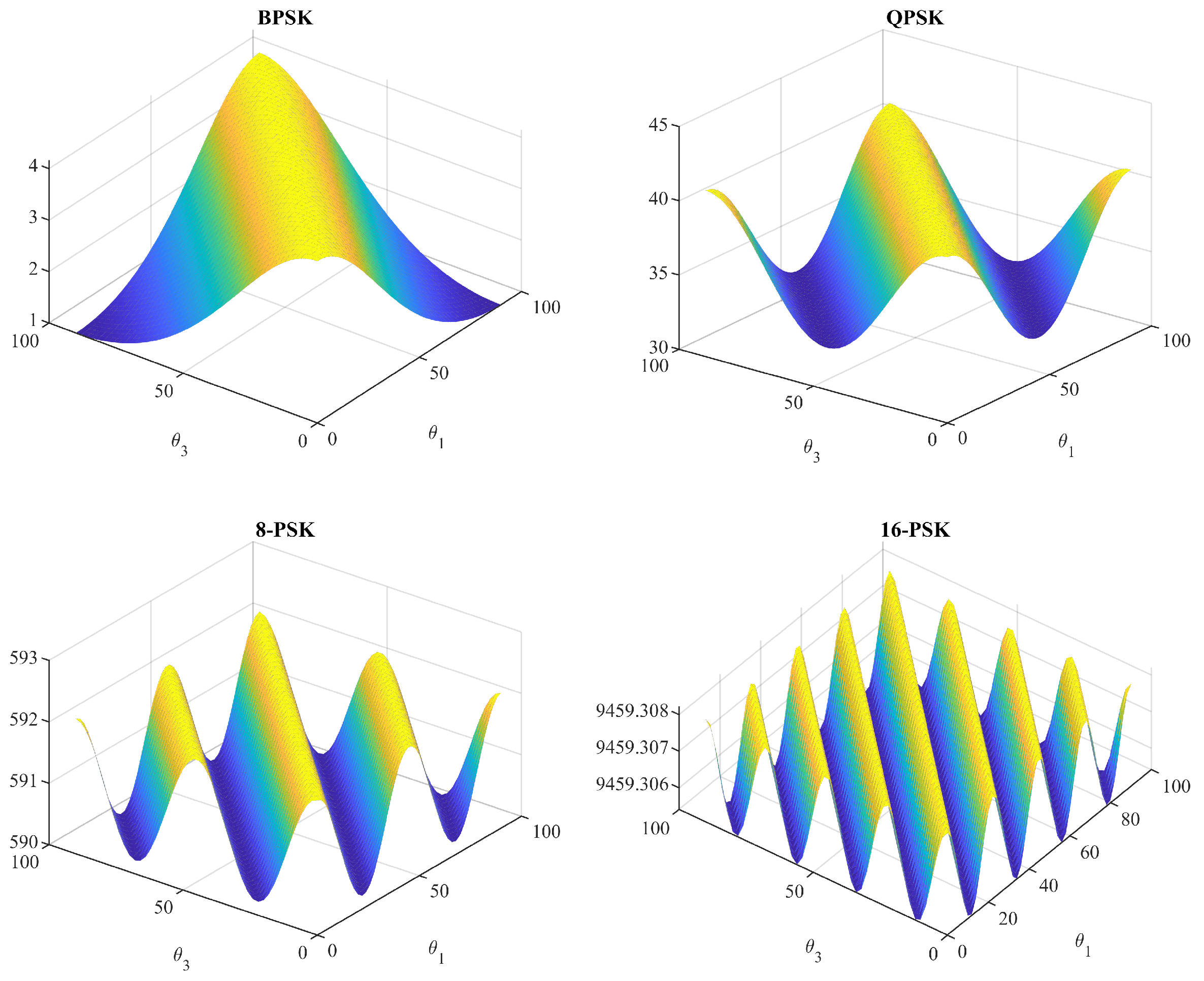
To verify the formula in (22), a three-dimensional graph is generated for four different PSK modulation schemes and illustrated in Figure 1. The value of the cost function depends on the difference between the angles rather than on individual values. As presented in Figure 1, we can conclude that the difference in the value of the cost function in (21) using the optimal angles and non-optimal angles vanishes as the modulation order increases.

Table 2. The value of the cost function in (21) for optimal angles and ${\theta }_i=0$ for several PSK modulation schemes and $n_R=3$.

Modulation	QPSK		8-PSK		16-PSK		32-PSK
$\theta$	optimal	${\theta }_i=0$	optimal	${\theta }_i=0$	optimal	${\theta }_i=0$	optimal	${\theta }_i=0$
Cost	32.8	41.2	590.2	592.2	9459.3	9459.3	1.5135 × 10${}^5$	1.5135 × 10${}^5$

depicts the minimum value of the cost function when the optimal angles are used and the maximum value of the cost function assuming ${\theta }_i=0$, $\forall i$ for several modulation schemes. The cost values are obtained using (21) by substituting the corresponding values of the rotation angles. For modulation orders 16 or higher, the value of the cost function becomes independent of the rotation angles. As shown in Figure 1, the change in the function’s value (y-axis value) is marginal for the case of 16-PSK.

The error performance of the MA-SM, assuming the whole set of $\Omega$ terms, is considered and analyzed using PSK modulation. ${\Omega }_6$ is simplified as follows:

$${\Omega }_6=L^4{4}^{-n_R}$$

(23)

Figure 2 depicts the weighted values of ${\Omega }_2-{\Omega }_5$, weighted by their corresponding frequency f, on the left y-axis and the value of ${\Omega }_1$ weighted by $f_1$ on the right y-axis. The x-axis represents the iteration number of the optimization process given in (21). The 8-PSK modulation is used for the generation of both graphs. The number of receive antennas is equal to 3 and 5 in the left and right sub-figure, respectively. Based on (13), the upper bound on the pairwise error probability depends on the weighted sum of the six $\Omega$ terms. When the optimization algorithm converges to the optimal solution for $n_R=3$, $f_1{\Omega }_1$ is about 6094 ($f_1$=4, ${\Omega }_1=1523.5$, from (15)) and $f_6{\Omega }_6=256$ ($f_6=4$ and ${\Omega }_6=64$, from (23)), and the sum of the terms that depend on the rotation angles is about 1180. Note that the values of $\Omega$ are obtained by substituting the values of the optimal rotation angles in (15)–(20) for any modulation set. Therefore, the error probability will be dominated by the terms that do not depend on the rotation angles. Further dominance is remarked as $n_R$ increases, where

$${\displaystyle \frac{f_1{\Omega }_1+f_6{\Omega }_6}{{\sum }_{i=2}^5{f}_i{\Omega }_i}}\approx 75.4,$$

From the previous analysis and for $n_R=5$, we conclude that:

• For a given modulation order, the effect of the rotation angle on the upper bound on the pairwise error probability vanishes as $n_R$ increases.
• For a given $n_R$, the effect of the rotation angle on the upper bound on the pairwise error probability vanishes as the modulation order increases.

It is therefore expected that the change in the rotation angles would have minimal impact, if any, on the error performance of the MA-SM system. The error performance is verified in Section 5 using simulations.

The optimization of the rotation angles is analyzed for the case when both signal symbols are drawn from the same L-QAM constellation with $L>4$. Based on the result of the optimization process, the optimal rotation angle is given as:

$$|{\theta }_1-{\theta }_3|=|{\theta }_2-{\theta }_4|={\displaystyle \frac{\pi }{4}},\mathrm{with}{\theta }_1={\theta }_2,{\theta }_3={\theta }_4$$

(24)

Equation (22) is satisfied only for $n_R$= 2 or 3. For $n_R$ = 4 and 6, we remarked that $|{\theta }_1-{\theta }_3|=|{\theta }_2-{\theta }_4|\approx {65}^{\circ }$ leads to a better performance than values in (22). Several other sets of angles that are not symmetric achieve similar performances.

Figure 3 depicts the weighted $\Omega$ terms that depend on the rotation angles on the left y-axis, and the weighted ${\Omega }_1$ on the right y-axis, versus the iteration number of the multi-objective optimization process. The value of ${\Omega }_6$ is neglected as it is much smaller than ${\Omega }_1$. For instance, ${\Omega }_1/{\Omega }_6$ approximately equals 72 for 64-QAM. Based on the depicted graphs, we can draw the same conclusion of PSK modulation that the error probability will be dominated by the terms that do not depend on the rotation angles. Therefore, the rotation angles would have negligible effect on the error performance.

Table 3. A comparison between the minimum value, maximum value, and the one corresponding to the angles in [20] of the cost function in (21) for 16 and 64-QAM with $n_R=3$.

Modulation	16-QAM			64-QAM
$\theta$	optimal	${\theta }_i=0$	[20]	optimal	${\theta }_i=0$	[20]
Cost	31195	35883	31313	1.4027 × 10${}^7$	1.5975 × 10${}^7$	1.4225 × 10${}^7$

presents a comparison between the value of the cost function in (21) using the optimal rotation angles suggested in [20] and the conventional system without rotation for 16 and 64-QAM schemes. For both scenarios, the optimal rotation angles minimize the cost function.

4.3. Analysis of the MA-SM Performance for Configuration III

Based on the last configuration in Table 1, the size of the set $\Gamma$ is equal to 8. Therefore, there are 64 codeword error events. The event ${\gamma }_i\leftrightarrow {\gamma }_i$, where the spatial symbol is received without error, is repeated eight times. This leads to a single $\Omega$ term, denoted by ${\Omega }_1$ in

Table 4. Selected partial list of the $\Omega$ terms obtained for configuration III.

Error Event	Expression
${\gamma }_i\leftrightarrow {\gamma }_i$	${\Omega }_1=\sum {\left(|s_{k_1}-s_{{\widehat{k}}_1}{|}^2+|s_{k_2}-s_{{\widehat{k}}_2}{|}^2+{|s_{k_3}-s_{{\widehat{k}}_3}|}^2\right)}^{-n_R}$
${\gamma }_1\leftrightarrow {\gamma }_2$	${\Omega }_2=\sum {\left(|s_{k_1}{e}^{j{\theta }_1}-s_{{\widehat{k}}_1}{e}^{j{\theta }_2}{|}^2+|s_{k_2}{e}^{j{\theta }_1}-s_{{\widehat{k}}_2}{e}^{j{\theta }_2}{|}^2+|s_{k_3}{|}^2+{\left|s_{{\widehat{k}}_3}\right|}^2\right)}^{-n_R}$
${\gamma }_1\leftrightarrow {\gamma }_8$	${\Omega }_8=\sum {\left(|s_{k_2}{e}^{j{\theta }_1}-s_{{\widehat{k}}_1}{e}^{j{\theta }_8}{|}^2+|s_{k_1}{|}^2+|s_{k_3}{|}^2+|s_{{\widehat{k}}_2}{{|}^2+s_{{\widehat{k}}_3}|}^2\right)}^{-n_R}$
${\gamma }_2\leftrightarrow {\gamma }_4$	${\Omega }_{10}=\sum {\left(|s_{k_1}{e}^{j{\theta }_2}-s_{{\widehat{k}}_1}{e}^{j{\theta }_4}{|}^2+|s_{k_3}{e}^{j{\theta }_2}-s_{{\widehat{k}}_3}{e}^{j{\theta }_4}{|}^2+|s_{k_2}{|}^2+{\left|s_{{\widehat{k}}_2}\right|}^2\right)}^{-n_R}$
${\gamma }_2\leftrightarrow {\gamma }_8$	${\Omega }_{12}=\sum {\left(|s_{k_2}{e}^{j{\theta }_2}-s_{{\widehat{k}}_1}{e}^{j{\theta }_8}{|}^2+|s_{k_3}{e}^{j{\theta }_2}-s_{{\widehat{k}}_2}{e}^{j{\theta }_8}{|}^2+|s_{k_1}{|}^2+{\left|s_{{\widehat{k}}_3}\right|}^2\right)}^{-n_R}$
${\gamma }_3\leftrightarrow {\gamma }_6$	${\Omega }_{16}=\sum {\left(|s_{k_1}{e}^{j{\theta }_3}-s_{{\widehat{k}}_1}{e}^{j{\theta }_6}{|}^2+|s_{k_3}{e}^{j{\theta }_3}-s_{{\widehat{k}}_3}{e}^{j{\theta }_6}{|}^2+|s_{k_2}{|}^2+{\left|s_{{\widehat{k}}_2}\right|}^2\right)}^{-n_R}$
${\gamma }_3\leftrightarrow {\gamma }_8$	${\Omega }_{19}=\sum {\left(|s_{k_2}{e}^{j{\theta }_3}-s_{{\widehat{k}}_1}{e}^{j{\theta }_8}{|}^2+|s_{k_3}{e}^{j{\theta }_3}-s_{{\widehat{k}}_3}{e}^{j{\theta }_8}{|}^2+|s_{k_1}{|}^2+{\left|s_{{\widehat{k}}_2}\right|}^2\right)}^{-n_R}$
${\gamma }_4\leftrightarrow {\gamma }_7$	${\Omega }_{21}=\sum {\left(|s_{k_2}{e}^{j{\theta }_4}-s_{{\widehat{k}}_2}{e}^{j{\theta }_7}{|}^2+|s_{k_1}{|}^2+|s_{k_3}{|}^2+|s_{{\widehat{k}}_1}{{|}^2+s_{{\widehat{k}}_3}|}^2\right)}^{-n_R}$
${\gamma }_5\leftrightarrow {\gamma }_6$	${\Omega }_{24}=\sum {\left(|s_{k_1}{e}^{j{\theta }_5}-s_{{\widehat{k}}_1}{e}^{j{\theta }_6}{|}^2+|s_{k_3}{e}^{j{\theta }_5}-s_{{\widehat{k}}_3}{e}^{j{\theta }_6}{|}^2+|s_{k_2}{|}^2+{\left|s_{{\widehat{k}}_2}\right|}^2\right)}^{-n_R}$
${\gamma }_6\leftrightarrow {\gamma }_8$	${\Omega }_{27}=\sum {\left(|s_{k_2}{e}^{j{\theta }_6}-s_{{\widehat{k}}_2}{e}^{j{\theta }_8}{|}^2+|s_{k_3}{e}^{j{\theta }_6}-s_{{\widehat{k}}_3}{e}^{j{\theta }_8}{|}^2+|s_{k_1}{|}^2+{\left|s_{{\widehat{k}}_1}\right|}^2\right)}^{-n_R}$
${\gamma }_7\leftrightarrow {\gamma }_8$	${\Omega }_{29}=\sum {\left(|s_{k_1}{e}^{j{\theta }_7}-s_{{\widehat{k}}_1}{e}^{j{\theta }_8}{|}^2+|s_{k_3}{e}^{j{\theta }_7}-s_{{\widehat{k}}_3}{e}^{j{\theta }_8}{|}^2+|s_{k_2}{|}^2+{\left|s_{{\widehat{k}}_2}\right|}^2\right)}^{-n_R}$

. Note that ${\Omega }_1$ is the only term that does not depend on the rotation angles. Also, since the probability of the error event ${\gamma }_i\leftrightarrow {\gamma }_j$ is equal to ${\gamma }_j\leftrightarrow {\gamma }_i$, there are 28 other $\Omega$ terms, each is repeated twice. Out of the 28 terms, 19 have a similar form to ${\Omega }_2$, where there are two terms of the squared Euclidean distance between two rotated signal symbols and two power terms of a signal symbol. The remaining nine terms include a single term of the squared Euclidean distance between two rotated signal symbols and four power terms, as in ${\Omega }_8$. Table 4 gives a partial list of the $\Omega$ expressions.

In Table 4, the term with more occurrences of the rotation angles has more impact on the end result of the optimization process. For instance, ${\Omega }_8$ is a function of only two rotation angles each with a single frequency. On the other hand, ${\Omega }_2$ is a function of ${\theta }_1$ and ${\theta }_2$, where each angle occurred twice. We can therefore conclude that ${\Omega }_2$ has more impact on the obtained optimal rotation angle that does ${\Omega }_8$.

Table 5. Examples of the obtained optimal rotation angles (in radians) for QPSK and 16-QAM and several $n_R$ values. The values cost (opt), cost ([20]), and cost (zeros) are the value of the sum in (13) using the obtained optimal rotation angles, the angles given in [20], and the all-zero angles, respectively.

	${\mathit{n}}_{\mathit{R}}=3$		${\mathit{n}}_{\mathit{R}}=4$		${\mathit{n}}_{\mathit{R}}=6$
	QPSK	16-QAM	QPSK	16-QAM	QPSK	16-QAM
${\theta }_1$	1.1771	1.4667	0.4331	0.9055	0.6323	0.4048
${\theta }_2$	0.6387	0.8141	0.9759	0.2574	0.0817	1.1770
${\theta }_3$	0.0371	0.3523	0.0	1.3668	1.0712	0.0069
${\theta }_4$	0.0360	0.3056	1.5708	1.3678	1.0670	0.0002
${\theta }_5$	0.4603	0.7271	1.1448	0.1505	1.4985	0.7996
${\theta }_6$	1.0035	1.2225	0.5966	1.0150	0.4838	0.3971
${\theta }_7$	0.7985	1.0842	0.8076	0.4401	0.2664	1.1897
${\theta }_8$	1.5519	0.0688	0.0591	0.7278	1.0031	0.7830
cost (opt)	2246.4	1.7022 × 10${}^7$	628.6	1.0412 × 10${}^7$	65.9	1.3906 × 10${}^7$
cost ([20]	2344.2	1.7218 × 10${}^7$	695.5	1.0720 × 10${}^7$	88.9	1.6092 × 10${}^7$
cost (zeros)	2674.6	1.8555 × 10${}^7$	920.7	1.4343 × 10${}^7$	168.3	4.3682 × 10${}^7$

shows the obtained optimal rotation angles for QPSK and 16-QAM and several values of receive antennas. The values of the cost function (the sum term in (13) with $B=29$, $f_1=8$, and $f_i=2$, for i = 2,⋯, 29) is also included using the optimal angles, the angles given in [20] and the all-zero angles. In all scenarios, the optimal rotation angles derived in this paper reduced the values of the cost function. We remarked that several sets of rotation angles produce almost the same value of the multi-objective cost function. Table 5 lists a single example. Unlike in the case of configuration I and II, it is difficult to obtain a closed-form expression for the rotation angles.

5. Simulation Results and Discussion

The effect of the rotation angles on the BER performance of the MA-SM system is evaluated for several system configurations. We adapted in this paper the same transmitter design in [20] in terms of the number of transmit antennas, the number of active transmit antennas at each channel use, the modulation schemes used for bit-to-symbol mapping, and the channel and noise models. The elements of the channel matrix and the noise vector are follow a cyclically symmetric Gaussian distribution with zero mean. The channel state information (CSI) is assumed to be perfectly known for the study of this paper. This is a general assumption in the literature when the channel estimation is not addressed in the provided work. This paper and [20] developed a baseband implementation of the communication system. We also assume that all signal symbols are drawn from the same modulation set.

Figure 4 depicts the performance of MA-SM with $N_T=4$, $N_P=2$ and several values of $n_R$. QPSK and 16-QAM are used to generate the results depicted in the left and right sub-figure, respectively. For both cases, we remarked that the performances of MA-SM using the optimal angles, the angles proposed in [20], and with the angles set to zero (without rotation) are identical for $n_R=$ 3 and 4. In the case of $n_R=6$, the BER performance of MA-SM using the optimal angles slightly outperforms the performance of the other two angle sets, especially in the case of QPSK. However, this improvement is marginal and barely noticeable.

Figure 5 depicts the performance of MA-SM with $N_T=5$, $N_P=3$ and several values of $n_R$. The performance of MA-SM using the three angle sets coincides for $n_R=3$. In the case of $n_R=4$, a slight improvement in the BER performance is remarked in the case of QPSK. At $n_R=6$, the performance of MA-SM with QPSK is improved due to the optimal rotation angle, and a slight improvement is also observed when 16-QAM is used. Again, the improvements in the BER using the 3-dimensional constellation are marginal and the MA-SM system can be used without applying any rotation to of the combinations while keeping the BER performance identical to that when the optimal rotation angles are applied. This paper developed a baseband implementation of the communication system. As a future work, we would like to implement the system using software-defined radio. This will permit the evaluation of the system under more realistic environment and taking into consideration system impairments.

6. Conclusions

The goal of this work is to validate the application of the 3-dimensional constellation that was introduced in the literature for the generalized SM with multiple active antennas (MA-SM). In this paper, we derived closed-form upper bound formulae of the pair-wise error probability of the MA-SM system as a function of the rotation angles used in the 3-dimensional constellation. To this end, the search problem is modeled as a multi-objective optimization. The obtained optimal set of angles are then evaluated against those which were proposed in the literature and the MA-SM system without the 3-dimensional constellation. We finally showed, using analytical and simulation results, that only a slight improvement of less than 0.5 dB in the error performance is achieved using the optimal angles. Therefore, we do not recommend the use of 3-dimensional constellation with the MA-SM system.

References

1. Ishikawa, N.; Sugiura, S.; Hanzo, L. 50 years of permutation, spatial and index modulation: From classic RF to visible light communications and data storage. IEEE Commun. Surv. Tutor. 2018, 20, 142–149. [Google Scholar] [CrossRef] [Green Version]
2. Mesleh, R.; Haas, H.; Sinanovic, S.; Ahn, C.; Yun, S. Spatial modulation. IEEE Trans. Veh. Technol. 2008, 57, 2228–2241. [Google Scholar] [CrossRef]
3. Jeganathan, J.; Ghrayeb, A.; Szczecinski, L.; Ceron, A. Space Shift Keying Modulation for MIMO Channels. IEEE Trans. Wirel. Commun. 2009, 8, 3692–3703. [Google Scholar]
4. Kaddoum, G.; Ahmed, M.F.A.; Nijsure, Y. Code Index Modulation: A High Data Rate and Energy Efficient Communication System. IEEE Commun. Lett. 2015, 19, 175–178. [Google Scholar]
5. Zhang, J.; Wang, Y.; Zhang, J.; Ding, L. Polarization Shift Keying (PolarSK): System Scheme and Performance Analysis. IEEE Trans. Veh. Technol. 2017, 66, 10139–10155. [Google Scholar] [CrossRef]
6. Basar, E.; Aygolu, U.; Panayirci, E.; Poor, H.V. Orthogonal Frequency Division Multiplexing With Index Modulation. IEEE Trans. Signal Process. 2013, 61, 5536–5549. [Google Scholar] [CrossRef]
7. Zhu, X.; Wang, Z.; Wang, Q.; Haas, H. Virtual Spatial Modulation for MIMO Systems. In 2016 IEEE Global Communications Conference (GLOBECOM); IEEE: Washington, DC, USA, 2016; pp. 1–6. [Google Scholar]
8. Li, J.; Wen, M.; Zhang, M.; Cheng, X. Virtual Spatial Modulation. IEEE Access 2016, 4, 6929–6938. [Google Scholar] [CrossRef]
9. Younis, A.; Mesleh, R.; Di Renzo, M.; Haas, H. Generalised spatial modulation for large-scale MIMO. In Proceedings of the 2014 22nd European Signal Processing Conference (EUSIPCO), Lisbon, Portugal, 1–5 September 2014; pp. 346–350. [Google Scholar]
10. Ju, P.; Zhang, M.; Cheng, X.; Wang, C.X.; Yang, L. Generalized spatial modulation with transmit antenna grouping for correlated channels. In Proceedings of the 2016 IEEE International Conference on Communications (ICC), Kuala Lamput, Malaysia, 22–27 May 2016. [Google Scholar]
11. AbuTayeh, S.; Alsalahat, M.; Kaddumi, I.; Alqannas, Y.; Althunibat, S.; Mesleh, R. A half-full transmit-diversity spatial modulation scheme. In Proceedings of the International Conference on Broadband Communications. Networks and Systems (BROADNETS), Faro, Portugal, 19–20 September 2018; pp. 257–266. [Google Scholar]
12. Mohaisen, M. Constellation design and performance analysis of the parallel spatial modulation. Int. J. Commun. Syst. 2019, 32, e4165. [Google Scholar]
13. Mesleh, R.; Ikki, S.S.; Aggoune, H.M. Quadrature Spatial Modulation. IEEE Trans. Veh. Technol. 2015, 64, 2738–2742. [Google Scholar]
14. Vo, B.; Nguyen, H.H. Improved Quadrature Spatial Modulation. In 2017 IEEE 86th Veh. Technol. Conference (VTC-Fall); IEEE: Toronto, ON, USA, 2017; pp. 1–5. [Google Scholar]
15. Holoubi, T.; Murtala, S.; Muchena, N.; Mohaisen, M. On the performance of improved quadrature spatial modulation. ETRI J. 2020. [Google Scholar] [CrossRef]
16. Yigit, Z.; Basar, E. Double Spatial Modulation: A High-Rate Index Modulation Scheme for MIMO Systems. In 2016 International Symposium on Wireless Communication Systems (ISWCS); IEEE: Poznan, Poland, 2016; pp. 347–351. [Google Scholar]
17. Mohaisen, M.; Lee, S. Complex Quadrature Spatial Modulation. ETRI J. 2017, 39, 514–524. [Google Scholar] [CrossRef]
18. Mohaisen, M. Increasing the Minimum Euclidean Distance of the Complex Quadrature Spatial Modulation. IET Commun. 2018, 12, 854–860. [Google Scholar] [CrossRef]
19. Iqbal, A.; Mohaisen, M.; Kwak, K.S. Modulation Set Optimization for the Improved Complex Quadrature SM. Wirel. Commun. Mobile Comput. 2018, 1–12. [Google Scholar] [CrossRef]
20. Wang, J.; Jia, S.; Song, J. Generalised Spatial Modulation System with Multiple Active Transmit Antennas and Low Complexity Detection Scheme. IEEE Trans. Wirel. Commun. 2012, 11, 1605–1615. [Google Scholar] [CrossRef]
21. Altın, G.; Çelebi, M.E. A Simple Low-Complexity Algorithm for Generalized Spatial Modulation. AEU Int. J. Electron. Commun. 2018, 97, 63–67. [Google Scholar] [CrossRef]
22. Zheng, B.; Wen, M.; Chen, F.; Huang, N.; Ji, F.; Yu, H. The K-Best Sphere Decoding for Soft Detection of Generalized Spatial Modulation. IEEE Trans. Commun. 2017, 65, 4803–4816. [Google Scholar] [CrossRef]
Figure 1. Three-dimensional graphs of the cost function in (21) as a function of θ 1 and θ 3 for BPSK, QPSK, 8-PSK, and 16-PSK modulation schemes and n R = 3 .
Applsci 10 03718 g001
Figure 2. The value of the weighted Ω terms that are affected by the rotation angle (left y-axis) and the value of the rotation-independent Ω 1 (right y-axis) for n R = 3 (left sub-figure) and n R = 5 (right sub-figure), assuming 8-PSK.
Applsci 10 03718 g002
Figure 3. The value of the weighted Ω terms that depend on the rotation angle (left y-axis) and the value of the rotation-independent Ω 1 (right y-axis) for n R = 3 and 16-QAM (left sub-figure) and 64-QAM (right sub-figure).
Applsci 10 03718 g003
Figure 4. BER of MA-SM using the optimal rotation angles, the angles derived in [20], and the all-zero angle set, for N T = 4 , N P = 2 , n R = 3, 4, and 6, using QPSK (left sub-figure) and 16-QAM (right-sub-figure).
Applsci 10 03718 g004
Figure 5. BER of MA-SM using the optimal rotation angles, the angles derived in [20], and the all-zero angle set, for N T = 5 , N P = 3 , n R = 3, 4, and 6, using QPSK (left sub-figure) and 16-QAM (right-sub-figure).
Applsci 10 03718 g005