RADIO: Parameterized Generative Radar Data Augmentation for Small Datasets

Abstract

We present a novel, parameterised radar data augmentation (RADIO) technique to generate realistic radar samples from small datasets for the development of radar-related deep learning models. RADIO leverages the physical properties of radar signals, such as attenuation, azimuthal beam divergence and speckle noise, for data generation and augmentation. Exemplary applications on radar-based classification and detection demonstrate that RADIO can generate meaningful radar samples that effectively boost the accuracy of classification and generalisability of deep models trained with a small dataset.

1. Introduction

Most autonomous vehicles currently rely on light detection and ranging (LiDAR) and camera technology to build their perception systems [1,2,3,4]. However, one of the main drawbacks of optical technology is failure under severe weather conditions such as fog, rain and snow. On the other hand, 24 GHz and 79 GHz radar systems have been widely adopted for adaptive cruise control and obstacle avoidance. Radar systems can penetrate bad weather [5], but the main drawback is their low resolution (e.g., ∼4 meter azimuth resolution at a 15 meter range [6]), which makes object classification and recognition very challenging.

Recent work on automotive radar has been aimed at improving azimuthal and range resolution at the 300 GHz frequency [5,7]. In previous work [8], we studied the performance of a number of neural network architectures applied to 300 GHz data for object detection and classification using a prototypical object set of six different objects in both isolated and multiple object settings. Our results were very much dependent on the different scenarios and objects, achieving accuracy ratings in excess of $90\%$ in the easier cases, but much lower success rates in a detection and classification pipeline with many confusing objects in the same scene. We do not rely on Doppler signatures [9,10,11] as we cannot consider only moving objects, nor do we use multiple views [12] to build a more detailed radar power map, as these are not wholly suited to the automotive requirement to classify both static and moving actors from a single view.

In our work—and indeed in the general literature—radar datasets tend to be small due to the difficulty of data collection and human annotation. While we endeavour to collect and label larger datasets in the wild, this is challenging due to the lack of advanced, high resolution automotive radars for high frame rate imaging, and the difficulty of radar image labelling in comparison with video sequences. Therefore, to create larger datasets to train deep models for such tasks, in this paper, we present a novel radar data augmentation technique which can be used for both classification and detection (Figure 1). Our experimental hypothesis is that such augmentation will improve the accuracy over standard camera-based data augmentation source data. Thus, the main contributions of this paper are as follows:

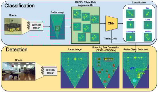
Figure 1. RADIO—radar data augmentation—is a data augmentation technique based on the physical properties of the radar data. The methodology is developed for both object detection and classification. CNN: convolutional neural network. DBSCAN: density-based spatial clustering of applications with noise.

• We present a novel radar data augmentation technique (RADIO) based on the measured properties of the radar signal. This models signal attenuation and resolution change over range, speckle noise and background shift for radar image generation.
• We demonstrate that such data augmentation can boost the accuracy and generalizability of deep models for object classification and detection, trained only with a small amount of source radar data. This verifies the effectiveness of the RADIO approach.

2. 300 GHz FMCW Radar

Current commercial vehicle radars use multiple input multiple output (MIMO) technology at 77–79 GHz with up to 5 GHz bandwidth and a very limited range—typically 35 cm—and azimuth resolution—typically 15° [6]. This equates to a cross range resolution of ≈4 m at 15 m, meaning that a car will occupy only one cell in the radar image. In this work, we use a 300 GHz frequency modulated continuous wave (FMCW) scanning radar designed by the University of Birmingham [13,14]. The assumed advantage of the increased resolution is a better radar image which may lead to more reliable object classification. The 300 GHz radar has a bandwidth of 20 GHz, which equates to a 0.75 cm range resolution. The azimuth resolution is 1.2°, which corresponds to 20 cm at 10 m. Figure 2 shows 300 GHz radar images with different bandwidths. As can be seen, the 20 GHz bandwidth provides much better resolution compared to current commercial sensors, and as such is considered for classification in this paper.

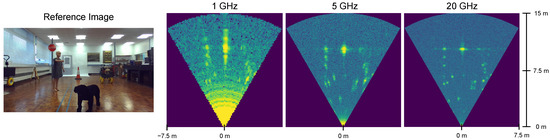
Figure 2. Images from the 300 GHz radar with different radar bandwidths. The data were collected at the University of Birmingham using the system described in [13].

The raw data captured by the 300 GHz radar comprise a time-domain signal at each azimuth direction. To transform the raw signal into an image, a Fast Fourier Transform (FFT) is applied to create a range profile at each azimuth, which is then converted to decibels (dB). The original polar image is converted to Cartesian coordinates to ensure consistent object dimensions at all ranges.

3. RADIO: Radar Data Augmentation

Using a restricted dataset, a DNN will easily overfit and be biased towards specific artifacts in the few examples the dataset provides. Our original experiments to recognise objects in 300 GHz radar data [8] had a database of only 950 examples at short range, as shown in Table 1. In this paper, we report a radar data augmentation technique to generate realistic data in which the neural network can learn patterns of data not present in the restricted source data and so avoid overfitting. Given the nature of radar signal acquisition and processing, the received power and azimuthal resolution vary with range and viewing angle. We also consider the effects of speckle noise and background shift during augmentation.

Table 1. Dataset collection showing the number of different raw images [8].

	Train 3.8 m	Test 6.3 m
Bike	90	90
Trolley	90	90
Mannequin	90	90
Cone	25	25
Traffic Sign	90	90
Stuffed Dog	90	90
Total	475	475

3.1. Attenuation

In the basic form of the radar equation, the power received by the radar transceiver [15] can be computed by

$$P_r=\frac{P_t{G}^2\sigma {\lambda }^4}{{\left(4\pi \right)}^3{R}^{4}L}$$

(1)

where $P_r$ is the received power, $P_t$ is the transmitted power, G is the antenna gain, $\sigma$ is the radar cross section (RCS), R is the range between the radar and the object, $\lambda$ is the radar wavelength and L is the loss factor. L can be atmospheric loss, fluctuation loss and/or internal attenuation from the sensor.

However, this assumes an idealised model in which a point—the isotropic radiator modified by the directional gain, G—propagates a radio signal that is reflected by a point scatterer in the far field at the same range, R. In practice, in our experiments, we use antennae of the order of 6 cm lateral dimension propagating at 300 GHz to extended targets in the range 3–12 m and simulate radar images in the range 2–15 m, as our operating range was constrained by the limited radar power and lab dimensions, meaning that we operated in the near field below the crossover point. Furthermore, for the precise theoretical computation of the received power, we would need information regarding the shape of the objects, placement of scatterer, surface material reflectivity and of multiple reflections caused by the surrounding walls, floor, ceiling and furniture [16]. Characterising the nature of point scatterer for real traffic actors such as vehicles is a very daunting task and is prone to error; simulation and measurement rarely correspond [17]. Our own data set is restricted, as shown in Figure 3, but there are still noticeable differences between, for example, the cone, which is a symmetrical plastic object, and the trolley, which is a collection of linear metallic struts and corners that act almost as ideal corner reflectors. Thus, as complete modelling is intractable, to augment our radar data, we have taken an empirical approach that measures the received power over pixels in the radar images as a function of range for all objects in our target set and therefore generates augmented radar image data at ranges not included in the real data using a regression fit to the actual data.

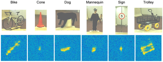
Figure 3. Samples from each object at 3.8 m from the dataset collected using the 300 GHz radar [8].

Figure 4 shows the measurements and the linear regression model for the six different objects (trolley, bike, stuffed dog, mannequin, sign and cone). To collect these data, we manually placed objects at different ranges and retrieved the mean received power intensity ($P_r$) from each object as a function of range. To compute $P_r$, the area of the image containing the object was cropped manually; then, a simple threshold was applied to remove background pixels. Simple thresholding is applicable to the training data as the object power levels are considerably higher than the background, which was at a consistent level at all ranges. Considering the collected data points, it appears that a reasonable approximation for variation of received power (dB) over range can be made by a linear regression between the received power and range, which is not predicted by Equation (1), which would suggest that the linear relationship should be over the logarithm of range. However, as we have noted, the basic equation makes many inapplicable assumptions; thus, we employ the empirical approximation in this scenario.

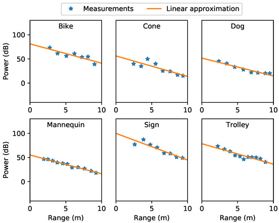
Figure 4. Received power as a function of range for all objects.

3.2. Change of Resolution

The next effect we consider is the change of resolution over range. The raw radar signal is in a polar coordinate system; when converting to Cartesian coordinates, interpolation is necessary to convert cells of irregular size as a function of range to uniformly spaced square cells (or pixels). Again, this means that the distribution of assumed point scatterers to cells might be quite different, and this is not measurable, as stated in Section 3.1. To account for the effect of changing Cartesian resolution with range, we determine the size of the polar cell at the range at which we wish to augment the radar data, and use nearest neighbor interpolation to generate the new Cartesian image. Figure 5 shows examples of trolley images generated at ranges from 2–15 m using this methodology and—as source data—the real range image at 3.8 m.

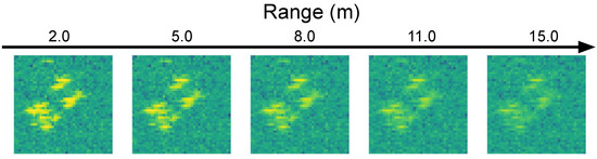
Figure 5. Range data augmented images for the trolley at 2–15 m.

To check whether the augmented data have similarity to real data and thus have some prospect of improving the training data, we compared the mean sum of absolute differences (MSAD) between real and augmented 3.8 m and 6.3 m images. As source data, we used the real 3.8 m image, but in this case we generated both a 3.8 m augmented image and a 6.3 m image from the source data and the regression curves in Figure 4. We used all samples with the same rotation for each class. The differences between the real and augmented images can be compared visually in Figure 6 and are also shown in Table 2. The low values for MSAD between the real and augmented images give us some confidence that the coupled attenuation and resolution procedures may be effective as an augmentation process throughout the range for training a neural network.

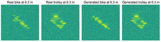
Figure 6. Comparing the real data at 6.3 m with the RADIO augmented data.

Table 2. Mean sum of absolute differences (MSAD) between the real and augmented images at 3.8 m and 6.3 m, generated from real data at 3.8 m only.

	Trolley	Bike	Cone	Mannequin	Sign	Dog
MSAD (3.8 m)	2.593	1.444	0.073	0.551	0.426	0.964
MSAD (6.3 m)	2.374	1.298	0.056	0.506	0.359	0.881

3.3. Speckle Noise and Background Shift

To further simulate real radar data, we included the capability to approximate the effects of different levels of speckle noise and background shift. Full modelling of speckle noise requires detailed knowledge of the properties of the radar system and antennae, but drawing on previous work [18], we performed an approximation by imposing multiplicative Gaussian noise, $I=I\ast \mathcal{N}(1,{\sigma }^2)$, where ${\sigma }^2$ is sampled uniformly from 0.01 to 0.15. Examples of speckle noise augmentation are given in Figure 7 with different multiplicative noise levels. As a final process, we also added background shift. This changes the brightness, creating scenes with objects and different background levels. It is a simple technique in which the constant false alarm rate (CFAR) is applied to the image, classifying the areas of the image as either object or background. A constant value is added/subtracted only to/from the background. Figure 8 shows examples of images with the application of background shift.

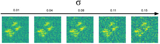
Figure 7. Speckle noise data augmentation.

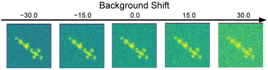
Figure 8. Background shift data augmentation.

4. Neural Network Architecture

We can formalize a neural network,

$$y=f(x^l;W^l)$$

(2)

where y is the output, f is the activation function, $W^l$ is a set of weights at layer l and $x^l$ is the input at layer l. The neural network learns the weights W which should be generalized to any input. Architectures may have several types of layers: convolutional, rectified linear units (ReLU), max pooling, dropout and softmax [19].

The neural network used in our work is A-ConvNet [20], shown in Table 3. We have implemented this network from the description in [20] using the PyTorch framework [21]. The only modification we have made is in the last layer with six convolution filters, which represents the number of classes for our classification. This architecture is fully convolutional and achieved state-of-the-art results for the MSTAR radar dataset [20]. The original input layer of A-Convnet is $88\times 88$, so our input data were re-sized using bilinear interpolation to fit the original model. To train our neural network, we used stochastic gradient descent (SGD). SGD updates the weights of the network depending on the gradient of the function that represents the current layer, as in Equation (3). In Equation (3), $\eta$ is the momentum, $\alpha$ is the learning rate, t is the current time step, W defines the weights of the network and $\nabla f(x;W)$ is the derivative of the function that represents the network. The chain rule was used to propagate the gradient through the network. The loss function was the categorical cross-entropy (Equation (4)), where $\widehat{y}$ is the predicted vector from the softmax output and y is the ground truth. We used 20% of the training radar data for validation, and the results were computed on the basis of the best results from the validation set.

$$W_{t+1}=W_t-\alpha \nabla f(x;W)+\eta \Delta W$$

(3)

$$L(\widehat{y},y)=-\sum _i{y}_{i}log\left({\widehat{y}}_i\right)$$

(4)

Table 3. A-ConvNet Architecture.

Input

Conv 16 ($5\times 5$) [ReLU]

MaxPool $2\times 2$

Conv 32 ($6\times 6$) [ReLU]

MaxPool $2\times 2$

Conv 64 ($6\times 6$) [ReLU]

MaxPool $2\times 2$

Dropout 0.5

Conv 128 ($5\times 5$) [ReLU]

Conv 6 ($3\times 3$) [Softmax]

Label Distribution

5. Experimental Results

The purpose of the experimental study is to verify the hypothesis that radar data augmentation will lead to the improved recognition of objects in radar images when compared to either the raw data alone or to data augmented by the “standard” techniques [19] commonly applied to visual image databases when training neural networks.

We have sub-divided these experiments into two main sets: in the first case, which we term “classification”, we consider images of isolated objects as both training and validation/test set data—this is a “per window” task; in the second case, we consider “detection” and “classification”, in which the training data are as before, but the test/validation data comprise a scene or image containing one or more instances of the known objects as well as the additional background— this is a “per image” task.

5.1. Classification

For classification, the single object dataset was acquired at 2 different ranges, 3.8 m and 6.3 m, with 360° rotations as shown in Table 1 and Figure 3. All the collected images were labelled with the correct object identity, irrespective of viewing range, angle and receiver height. A fixed size bounding box of $400\times 400$ cells, which corresponds to 3 m${}^2$, was cropped with the object in the middle. As stated above, the original images were resized to the $88\times 88$ input layer, and we used stochastic gradient descent (SGD) with the parameters shown in Table 4.

Table 4. Neural Network Parameters.

Learning rate ($\alpha$)	0.001
Momentum ($\eta$)	0.9
Epochs	100
Batch size	100

To test the hypothesis that principled data augmentation by RADIO improves on the commonly used, image-inspired data augmentation techniques, we conducted a series of experiments, as shown in Table 5. The standard data augmentation (SDA) techniques for image data that we employed are random translations and image mirroring [22]. Random translations changes the object location over the image, reducing the contribution of the background during the learning process. Rotations are not used because we already have data at all angles in the image plane. Although RGB image augmentation may include colour changes—i.e., modifying the colour map—this has no equivalent in the radar data, which are monochromatic, and this type of augmentation is therefore not applied. To ensure comparability of results, we applied the same number of camera-based data augmentations to each sample, meaning that each dataset is of similar size, as shown in Table 5. From Table 1, we have 475 samples for training, and we decided to employ the data augmentation methods 41 times for each sample, resulting in a total of 19,475 artificially generated samples and 19,950 in total. In Table 5, range data augmentation includes both attenuation and change of resolution ranges between 1 and 12 m, the addition of speckle noise with $\sigma$ [0.01 0.15], and four levels of background shift, as described in Section 3. To verify the use of RADIO augmentation at different ranges, and to avoid overfitting to range-specific features, we used the images from 3.8 m to train and the images from 6.3 m to test.

Table 5. Results for the single-object classification task. SDA = standard (RGB) data augmentation, RDA = range data augmentation, SN = addition of speckle noise, BS = background shift.

	Samples	Precision (%)	Recall (%)	F1-Score (%)	Accuracy (%)
Original Data	475	33.36	39.15	31.39	39.15
Original Data + SDA	19,950	80.71	82.13	79.49	82.13
Original Data + SDA + SN + BS (Ours)	19,950	88.51	83.83	82.42	83.83
Original Data + SDA + RDA + BS (Ours)	19,950	95.28	94.89	94.45	94.89
Original Data + SDA + RDA + SN + BS (Ours)	19,950	99.79	99.79	99.79	99.79

We used precision ($\frac{TP}{TP+FP}$), recall ($\frac{TP}{TP+FN}$), F-1 score ($2\times \frac{precision\times recall}{precision+recall}$) and accuracy ($\frac{TP+FN}{TP+TN+FP+FN}$) as metrics, where T is true, F is false, P is positive and N is negative.

The key observation from Table 5 is that the progressive augmentation of the training data by the RADIO methods leads to progressively improved scores according to all the commonly used metrics. The key comparison is between the second and fifth row of the table, in which equally sized training datasets were used, but the use of the radar adapted augmentation leads to an improvement from ≈80% to 99.79%. The only mistake is between the sign and the mannequin, as both have a very similar shape signature. Admittedly, this improvement is in a relatively easy scenario, as the object location is pre-defined in a classification window. In Section 5.2 we address a more challenging scenario in which multiple objects are seen in a laboratory setting with potential occlusion and mutual interference, and there is additional background clutter caused by unknown artefacts.

5.2. Detection and Classification

In this more realistic scenario, we have developed a dataset that contains several different scenes with several objects viewed against a background containing walls as a significant feature. Thus, the scene data include examples of occluded objects, multi-path reflection and interference between objects (Figure 9). This new dataset contains the same objects (bike, trolley, cone, mannequin, sign, dog) in different parts of the room with arbitrary rotations and ranges. We also include different types of mannequin, cone, trolley, traffic sign, and bikes, meaning that those objects can have different radar signatures. This new dataset contains 198 scenes and 648 objects, with an average of 3.27 objects per scene. In summary, we have 85 examples of bikes, 189 of trolleys, 132 of mannequins, 63 of cones, 129 of signs and 50 of stuffed dogs. Some examples of scene data are shown in Figure 10.

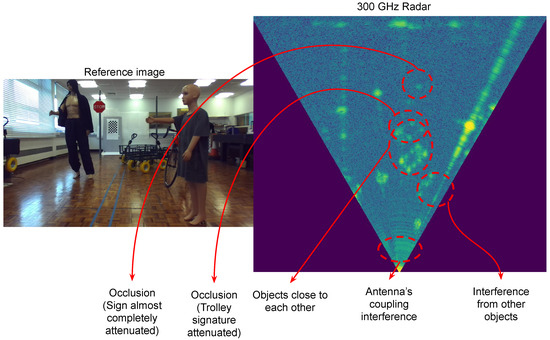
Figure 9. Possible unwanted effects in the multiple object dataset.

Figure 10. Qualitative results using RADIO for perfect detection, the constant false alarm rate (CFAR) + DBSCAN + network pipeline, and the corresponding video images.

To apply detection and classification, we developed a two-stage methodology similar to R-CNN [23], shown in Figure 1. First, we detect potential regions of interest and then classify each detected region. The CA-CFAR (cell-averaging constant false alarm rate) detection method [24] employs an adaptive threshold based on the statistics of the region to decide whether the return is of sufficient power to be of interest. In our implementation, this was applied to the original polar image at each azimuth direction. The empirically chosen parameters used for CFAR were 500 for cell size, 30 for guard cells and 0.22 for false alarm rate. Following detection, the standard density-based spatial clustering of applications with noise (DBSCAN) [25] technique was used to form a cluster of cells and remove outliers. The parameters used for DBSCAN were also selected empirically: $ϵ=0.3$ m, which is the maximum distance of separation between two detected points, and $S=40$, where S is the minimum number of points to form a cluster. We then generate fixed size bounding boxes of size $275\times 275$—the same size as the input from the single object images. Then, the image is resized to $88\times 88$ as before.

It is important to separate the effects of detection (by CFAR and clustering) from object classification (using the neural network); therefore, we perform two types of experiment, first, assuming perfect detection, and second, including the entire detection and classification pipeline. Thus, in the perfect detection case, the exact object location is known, and the unknown element is whether the classifier can still determine the correct object identity in the presence of the additional artefacts described above, bearing in mind that the network has been trained on the isolated objects, not the objects in the multiple object scenarios, and hence cannot learn any features that arise in that instance. As in the single object classification case, the key hypothesis is that the radar augmentation technique will give improved results when compared to the standard, optical image-derived methods.

In our experiments, we classified our scenes with regard to the number of objects and at short, mid and long ranges. Extensive results are shown in Table 6 and Table 7. We anticipated that, with more objects in the scene and at a greater distance, the effects of attenuation and mutual interference will cause the classification rates to fall. The metric for evaluation is average-precision (AP), which is used commonly in an object detection scenario. We use the PASCAL VOC implementation [26] with an intersection over union (IoU) equal to $0.5$. AP is computed as $AP={\int }_0^{1}p\left(r\right)dr$, where p is precision and r is recall. We retrained the neural network from the single object dataset using both ranges (3.8 m and 6.3 m) and tested on this new more realistic scenario. All the other parameters were the same. We applied the same data augmentation methods as before. We compared the standard data augmentation (SDA) with RADIO (SDA + RDA + SN + BS). There are several key observations to be made from these experiments. First, the results in all cases are significantly poorer than in the isolated object case, even for perfect detection, as we would expect as the data are much more challenging and realistic. For example, the overall mAP for perfect detection is only 66.28%. The second conclusion is that there are significant object differences. As ever, the easy task is to recognise the trolley, with an mAP of 90.08% in the perfect case, as opposed to the mannequin at 41.15% which is often confused with the cone for example. Third, we observe that, as expected, the type of scene has a significant effect. For example, in the perfect case, the overall mAP for less than four objects is 85.13% but this drops to 52.74% for more than seven objects. Similarly, for $4<7$ objects, the mAP drops from 79.09% to 66.58% as we move from short to long range, but the optimal scenario is often at middle range. This is probably attributable to stronger multipath effects at the shorter range, but this would require further examination. Regarding the cone object, we realised that the reflection of the cone, especially for long ranges, can get completely attenuated with values close to the background level, achieving worse results between sensed objects.

Table 6. Perfect detection: in white, the standard data augmentation is shown; in gray, our RADIO technique. The entry N/A means that there were no examples in the dataset.

AP	Overall	$\#\mathit{Objects}<4$				$4\le \#\mathit{Objects}<7$				$\#\mathit{Objects}\ge 7$				Short	Mid	Long
		Overall	Short	Mid	Long	Overall	Short	Mid	Long	Overall	Short	Mid	Long
bike	65.78	81.7	50.0	88.89	75.0	53.82	0.0	59.92	66.67	66.36	N/A	67.2	N/A	25.0	69.31	71.43
bike (ours)	71.94	90.98	50.0	94.44	100.0	64.55	100.0	59.99	100.0	53.43	N/A	48.92	N/A	75.0	67.17	100.0
cone	42.29	51.25	50.0	61.11	50.0	66.44	65.08	83.33	28.57	34.35	62.5	42.5	23.19	60.44	52.71	24.22
cone (ours)	49.96	66.67	50.0	66.67	100.0	69.23	66.67	66.67	83.33	35.07	62.5	13.33	0.0	62.07	37.04	45.31
dog	26.72	45.07	55.56	47.32	30.95	25.22	33.33	36.67	16.67	13.68	50.0	N/A	7.5	48.0	38.33	9.44
dog (ours)	67.26	86.43	88.89	99.05	11.11	64.74	83.33	60.42	50.0	30.91	40.0	N/A	0.0	68.0	85.02	6.67
mannequin	42.05	71.28	53.33	87.02	55.56	28.3	42.42	34.18	7.5	44.47	14.29	58.82	19.25	34.72	54.16	14.94
mannequin (ours)	41.15	82.61	83.33	92.86	33.33	28.56	45.45	26.67	14.55	36.28	14.29	52.94	10.92	45.83	49.94	10.62
sign	49.36	41.3	0.0	44.71	40.0	59.77	N/A	62.5	57.89	40.35	N/A	41.94	38.46	0.0	50.57	49.28
sign (ours)	77.26	87.01	100.0	90.09	66.67	74.49	N/A	80.19	70.27	76.92	N/A	77.78	76.19	100.0	82.52	72.13
trolley	84.61	90.23	84.72	99.92	76.47	87.35	100.0	91.66	68.81	78.51	95.99	85.78	26.67	96.29	91.69	61.94
trolley (ours)	90.08	97.08	97.62	99.44	94.12	94.16	100.0	96.42	81.36	83.82	100.0	87.79	44.37	99.01	92.91	75.11
ine mAP	51.80	63.47	48.94	71.49	54.66	53.48	48.17	61.38	41.02	46.29	55.69	59.25	23.01	44.07	59.46	38.54
mAP (ours)	66.28	85.13	78.31	90.43	67.54	65.96	79.09	65.06	66.58	52.74	54.2	56.15	26.3	74.99	69.1	51.64

Table 7. Constant false alarm rate detection and DBSCAN clustering followed by neural network classification.

AP	Overall	$\#\mathit{Objects}<4$				$4\le \#\mathit{Objects}<7$				$\#\mathit{Objects}\ge 7$				Short	Mid	Long
		Overall	Short	Mid	Long	Overall	Short	Mid	Long	Overall	Short	Mid	Long
bike	54.97	81.96	50.0	71.83	100.0	57.49	50.0	59.69	33.33	29.82	N/A	32.47	N/A	50.0	52.07	71.43
bike (ours)	70.60	88.55	70.0	74.16	100.0	63.75	100.0	57.3	66.67	61.13	N/A	58.92	N/A	78.85	61.66	83.67
cone	12.95	45.45	62.5	25.0	0.0	41.72	55.56	66.67	0.0	1.07	0.0	1.39	0.0	25.17	13.06	0.0
cone (ours)	18.41	27.27	25.0	16.67	0.0	45.1	55.56	50.0	0.0	2.94	0.0	6.67	0.0	18.72	17.9	0.0
dog	18.76	36.83	66.67	43.17	4.17	17.86	33.33	21.43	0.0	8.68	40.0	N/A	1.56	48.0	27.29	1.28
dog (ours)	58.74	77.88	77.78	98.08	5.56	50.51	66.67	44.44	0.0	33.75	48.33	N/A	0.0	63.53	74.81	1.54
mannequin	41.14	72.6	64.0	85.87	44.44	21.64	29.09	28.39	9.41	48.54	0.0	61.76	34.81	27.83	52.93	18.67
mannequin (ours)	39.49	87.18	100.0	92.86	44.44	26.0	36.36	23.33	19.23	33.65	0.0	50.0	13.33	39.13	47.27	15.3
sign	46.26	43.43	0.0	44.71	50.0	50.87	N/A	54.11	45.6	43.32	N/A	37.72	50.0	0.0	44.78	47.81
sign (ours)	72.67	88.22	100.0	91.93	66.67	71.94	N/A	78.05	65.25	69.51	N/A	65.24	78.36	50.0	76.82	68.43
trolley	80.03	83.94	68.33	94.36	73.12	84.18	97.44	88.26	64.48	74.47	79.56	75.54	34.0	82.82	83.87	59.2
trolley (ours)	82.75	81.06	84.72	88.37	64.46	88.66	95.6	92.89	68.35	82.1	87.41	80.15	45.24	88.19	84.48	58.0
ine mAP	42.35	60.7	51.92	60.82	45.29	45.63	53.08	53.09	25.47	34.32	29.89	41.78	24.08	38.97	45.67	33.06
mAP (ours)	57.11	75.02	76.25	77.01	46.85	57.66	59.03	57.66	36.58	47.18	22.62	43.49	22.82	56.40	60.49	37.82

As one might expect, the results of the detection classification pipeline are worse across the board in all cases, culminating in an overall figure of 57.11% as opposed to 66.28%. However, bearing in mind the key hypothesis, the most important result is the comparison of the results with RADIO (in gray) as opposed to standard argumentation techniques. Although there is an occasional anomaly, in almost all cases, the RADIO technique is shown to be an improvement over standard augmentation techniques. Again, looking at the overall figures, the mAP improves from 51.80% to 66.28% for perfect detection, and from 42.35% to 57.11% in the pipelined case.

6. Conclusions

In this paper, we proposed and investigated a radar data augmentation method (RADIO) and compared it to standard augmentation methods to see if this would lead to higher object classification rates in both isolated object and multi-object scenes. We were able to show that the use of radar data augmentation did indeed give improved results, and this offers a useful avenue to train a neural network when the source data are limited and the network cannot be trained under all the eventual test and validation conditions. In the absence of augmentation, using only the original data, overfitting is probable and the network cannot generalise.

In the isolated object case, after data augmentation, an accuracy of 99.79% was achieved. RADIO created realistic samples which helped the neural network to achieve near perfect recognition. In the more challenging multiple object dataset, we achieved 66.28% mAP for perfect detection and 57.11% mAP for the easy detection and classification scenario, in which the possible effects of multi-paths, objects in close proximity, antenna coupling, and clutter from unwanted objects are more challenging. Compared to standard camera based data augmentation, the RADIO technique gives improved results.

To develop further, it is necessary to improve detection, as this gives rise to additional errors in comparison with perfect detection; furthermore, it is necessary to extend the work to the more challenging scenarios of data collected “in the wild”. In the latter case, it is probable that both the training and test/validation data will be collected in wild conditions, as the differences between lab-based and outside data would be too great. To that end, we are currently collecting and processing data collected from a 79 GHz radar system mounted on a mobile vehicle.

References

- Premebida, C.; Carreira, J.; Batista, J.; Nunes, U. Pedestrian Detection Combining RGB and Dense Lidar Data. In Proceedings of the 2014 IEEE/RSJ International Conference on Intelligent Robots and Systems, Chicago, IL, USA, 14–18 September 2014; pp. 4112–4117. [Google Scholar]
- Du, X.; Ang, M.H.; Karaman, S.; Rus, D. A general Pipeline for 3D Detection of Vehicles. In Proceedings of the 2018 IEEE International Conference on Robotics and Automation (ICRA), Brisbane, Australia, 21–25 May 2018; pp. 3194–3200. [Google Scholar]
- Yang, F.; Choi, W.; Lin, Y. Exploit All the Layers: Fast and Accurate CNN Object Detector with Scale Dependent Pooling and Cascaded Rejection Classifiers. In Proceedings of the IEEE Conference on Computer Vision and Pattern Recognition, Las Vegas, NV, USA, 27–30 June 2016; pp. 2129–2137. [Google Scholar]
- Liang, M.; Yang, B.; Chen, Y.; Hu, R.; Urtasun, R. Multi-Task Multi-Sensor Fusion for 3D Object Detection. In Proceedings of the IEEE Conference on Computer Vision and Pattern Recognition, Long Beach, CA, USA, 15–20 June 2019; pp. 7345–7353. [Google Scholar]
- Daniel, L.; Phippen, D.; Hoare, E.; Stove, A.; Cherniakov, M.; Gashinova, M. Low-THz Radar, Lidar and Optical Imaging Through Artificially Generated Fog. In Proceedings of the International Conference on Radar Systems (Radar 2017), Belfast, UK, 23–26 October 2017; pp. 1–4. [Google Scholar]
- Texas Instruments. Short Range Radar Reference Design Using AWR1642; Technical Report; Texas Instruments: Dallas, TX, USA, 2017. [Google Scholar]
- Marchetti, E.; Du, R.; Willetts, B.; Norouzian, F.; Hoare, E.G.; Tran, T.Y.; Clarke, N.; Cherniakov, M.; Gashinova, M. Radar cross-section of pedestrians in the low-THz band. IET Radar Sonar Navig. 2018, 12, 1104–1113. [Google Scholar] [CrossRef]
- Sheeny, M.; Wallace, A.; Wang, S. 300 GHz Radar Object Recognition based on Deep Neural Networks and Transfer Learning. IET Radar Sonar Navig. 2020. [Google Scholar] [CrossRef]
- Rohling, H.; Heuel, S.; Ritter, H. Pedestrian detection procedure integrated into an 24 GHz automotive radar. In Proceedings of the 2010 IEEE Radar Conference, Washington, DC, USA, 10–14 May 2010; pp. 1229–1232. [Google Scholar]
- Bartsch, A.; Fitzek, F.; Rasshofer, R. Pedestrian Recognition Using Automotive Radar Sensors. Adv. Radio Sci. 2012, 10. [Google Scholar] [CrossRef]
- Angelov, A.; Robertson, A.; Murray-Smith, R.; Fioranelli, F. Practical Classification of Different Moving Targets Using Automotive Radar and Deep Neural Networks. IET Radar Sonar Navig. 2019, 12, 1082–1089. [Google Scholar] [CrossRef]
- Lombacher, J.; Laudt, K.; Hahn, M.; Dickmann, J.; Wöhler, C. Semantic Radar Grids. In Proceedings of the 2017 IEEE Intelligent Vehicles Symposium (IV), Los Angeles, CA, USA, 11–14 June 2017; pp. 1170–1175. [Google Scholar]
- Phippen, D.; Daniel, L.; Gashinova, M.; Stove, A. Trilateralisation of Targets Using a 300 GHz Radar System. In Proceedings of the International Conference on Radar Systems, Belfast, UK, 23–26 October 2017. [Google Scholar]
- Marchetti, E.; Daniel, L.; Hoare, E.; Norouzian, F.; Cherniakov, M.; Gashinova, M. Radar Reflectivity of a Passenger Car at 300 GHz. In Proceedings of the 19th IEEE International Radar Symposium (IRS), Bonn, Germany, 20–22 June 2018; pp. 1–7. [Google Scholar] [CrossRef]
- Radar Tutorial. 2019. Available online: https://www.radartutorial.eu/index.en.html (accessed on 14 October 2019).
- Knott, E.F.; Schaeffer, J.F.; Tulley, M.T. Radar Cross Section; SciTech Publishing: Raleigh, NC, USA, 2004. [Google Scholar]
- Schuler, K.; Becker, D.; Wiesback, W. Extraction of Virtual Scattering Centers of Vehicles by Ray-tracing Simulations. IEEE Trans. Antennas Propag. 2008, 56, 3543–3551. [Google Scholar] [CrossRef]
- Ding, J.; Chen, B.; Liu, H.; Huang, M. Convolutional Neural Network with Data Augmentation for SAR Target Recognition. IEEE Geosci. Remote Sens. Lett. 2016, 13, 364–368. [Google Scholar] [CrossRef]
- Goodfellow, I.; Bengio, Y.; Courville, A. Deep Learning; The MIT Press: Cambridge, MA, USA, 2016. [Google Scholar]
- Chen, S.; Wang, H.; Xu, F.; Jin, Y.Q. Target Classification Using the Deep Convolutional Networks for SAR Images. IEEE Trans. Geosci. Remote Sens. 2016, 54, 4806–4817. [Google Scholar] [CrossRef]
- Paszke, A.; Gross, S.; Chintala, S.; Chanan, G.; Yang, E.; DeVito, Z.; Lin, Z.; Desmaison, A.; Antiga, L.; Lerer, A. Automatic Differentiation in PyTorch. In Proceedings of the NIPS Autodiff Workshop, Long Beach, CA, USA, 9 December 2017. [Google Scholar]
- Jung, A.B.; Wada, K.; Crall, J.; Tanaka, S.; Graving, J.; Yadav, S.; Banerjee, J.; Vecsei, G.; Kraft, A.; Borovec, J.; et al. Imgaug. 2019. Available online: https://github.com/aleju/imgaug (accessed on 25 September 2019).
- Girshick, R.; Donahue, J.; Darrell, T.; Malik, J. Rich Feature Hierarchies for Accurate Object Detection and Semantic Segmentation. In Proceedings of the IEEE Conference on Computer Vision and Pattern Recognition, Columbus, OH, USA, 23–28 June 2014; pp. 580–587. [Google Scholar]
- Richards, M. Fundamentals of Radar Signal Processing; McGraw-Hill Education (India) Pvt Limited: Noida, India, 2005. [Google Scholar]
- Ester, M.; Kriegel, H.P.; Sander, J.; Xu, X. A Density-based Algorithm for Discovering Clusters a Density-based Algorithm for Discovering Clusters in Large Spatial Databases with Noise. In Proceedings of the Second International Conference on Knowledge Discovery and Data Mining, KDD’96, Portland, OR, USA, 2–4 August 1996; pp. 226–231. [Google Scholar]
- Everingham, M.; Eslami, S.A.; Van Gool, L.; Williams, C.K.; Winn, J.; Zisserman, A. The pascal visual object classes challenge: A retrospective. Int. J. Comput. Vis. 2015, 111, 98–136. [Google Scholar] [CrossRef]
© 2020 by the authors. Licensee MDPI, Basel, Switzerland. This article is an open access article distributed under the terms and conditions of the Creative Commons Attribution (CC BY) license (http://creativecommons.org/licenses/by/4.0/).