Deep Image Compression with Residual Learning

Abstract

An end-to-end image compression framework based on deep residual learning is proposed. Three levels of residual learning are adopted to improve the compression quality: (1) the ResNet structure; (2) the deep channel residual learning for quantization; and (3) the global residual learning in full resolution. Residual distribution is commonly a single Gaussian distribution, and relatively easy to be learned by the neural network. Furthermore, an attention model is combined in the proposed framework to compress regions of an image with different bits adaptively. Across the experimental results on Kodak PhotoCD test set, the proposed approach outperforms JPEG and JPEG2000 by PSNR and MS-SSIM at low BPP (bit per pixel). Furthermore, it can produce much better visual quality. Compared to the state-of-the-art deep learning-based codecs, the proposed approach also achieves competitive performance.

1. Introduction

Image compression is a fundamental and well-studied problem in the data compression field. Typical conventional compression algorithms such as JPEG [1] and JPEG2000 [2] are based on transform coding theory [3]. JPEG adopts the discrete cosine transform (DCT) while JPEG2000 adopts the discrete wavelet transform (DWT) to convert an original image into a latent compression representation space.

Recently, lossy image compression frameworks based on deep learning (DL) have raised interest in both deep learning and image processing communities [4,5,6,7,8,9,10]. Although these approaches are competitive with the existing modern engineered codecs such as JPEG [1], JPEG2000 [2], WebP [11], and BPG [12], several issues and challenges still need to be addressed. Firstly, existing learning methods commonly compress the full resolution image at one-shot regardless of the difference between high- and low-frequency information, which brings out some artifacts and block effects. Secondly, data compression is mainly reflected in the quantization stage, but it may introduce too many unnecessary errors. Based on previous works, a residual learning framework is proposed by introducing some novel technologies to properly improve the compression quality.

In Section 1.1, DL-based image compression related works are reviewed and discussed. In Section 1.2, deep channel residual learning is introduced. In Section 1.3, global residual learning in full resolution is presented. In Section 1.4, the main contributions of this paper are summarized.

1.1. DL-Based Image Compression and Related Works

Generally, a typical end-to-end lossy image compression framework can be formulated as jointly optimizing all modules: an encoder $E_{\varphi }$, a quantizer Q, a decoder $D_{\theta }$, and some other rate estimation and rate-distortion control module R, where $\varphi$ and $\theta$ are the trained weights.

$$E_{\varphi }:{\mathbb{R}}^N\to {\mathbb{R}}^M\hspace{1em}{D}_{\theta }:{\mathbb{R}}^M\to {\mathbb{R}}^N\hspace{1em}Q:{\mathbb{Z}}^M\to [0,1]$$

(1)

A vector of image intensities $x\in {\mathbb{R}}^N$ is mapped to a latent presentation space $y\in {\mathbb{R}}^M$ via the encoder $E_{\varphi }$, $y=E_{\varphi }\left(x\right)$. y is quantized into a discrete-valued vector $\widehat{q}\in Z^M$ via the quantizer Q. The entropy rate of the vector $\widehat{q}$ is estimated and minimized via R. The reconstructed image can be represented as $\tilde{x}$ = $D_{\theta }$($\tilde{q}$). Distortion is often assessed by the distance between x and $\tilde{x}$, $D(x,\tilde{x}$), namely PSNR (Peak Signal to Noise Ratio), or the perceptual measure such as MS-SSIM (Multi-scale Structural Similarity) [13]. Rate estimation is often assessed by the minimal entropy of the discrete bit streams. Therefore, image compression is typically formulated as a distortion and rate optimization problem. The goal is o optimize the trade-off between using a minimal number of bits and having minimal distortion.

$$Optimizationobject:\underset{Distortion}{\underbrace{D(x,\tilde{x})}}-\lambda ·\underset{Numberofbits}{\underbrace{lo{g}_{2}Q\left(E_{\varphi }\left(x\right)\right)}}$$

(2)

Existing DL-based image compression frameworks are mainly classified into the auto-encoder and recurrent neural network (RNN). In the case of auto-encoder, recent works have focused on variational Bayes and autoregressive context methods to develop accurate entropy estimation models by optimizing the R-D curve and introducing hyper prior parameters [6,8]. The prior probability of compression representation is modeled by a Gaussian or Laplacian distribution by an underlying auto-encoder. Since the Lagrange multiplier $\lambda$ is introduced as a hyper-parameter for a desired trade-off between the rate and distortion, it is not efficient and different models must be trained for different compression rates.

Due to a large fraction of Internet traffic driven by requests from mobile devices, a progressive algorithm is more popular. Recurrent neural networks (RNNs)-based frameworks only need to be trained once to produce a progressive and variable-rate model, regardless of the desired compression rate [14,15]. However, the RNN-based methods require multiple iterations to obtain high-quality images. Besides, Agustsson et al. [4] proposed a generative adversarial network to obtain visually pleasing results at low bit rates where previous methods fail and show strong artifacts. Although the PSNR and MS-SSIM index shows no advantage, the reconstructed images seem better than others at extremely low bit rates.

Combined with the advantages of both, the proposed framework adopts the recurrent architecture with rate control to learn residual information.

1.2. Deep Channel Residual Learning

Since quantization is necessary for compression, it also introduces a lot of errors. Assuming that the shape of the quantized bits is $n\times h\times w$, the quantization errors exist in these coded bits. Motivated by denoising algorithm in traditional signal processing, a variation of $\Delta \mathsf{\Sigma }$ modulation similar to residual learning is introduced. Utilizing the residual information between the adjacent channel can eliminate errors effectively. Given the input is x, the quantizer is $sign$ function, and the quantized bits is $\widehat{q}$. The residual is r, i.e. the difference between current channel $y_i$ and previous quantized channel $\widehat{q_i}$. The reconstruction z is accumulated by residual r. The errors existed between channels can be eliminated in the process of calculating the residual and accumulation of the information. The specific process of channel residual learning is depicted as Algorithm 1.

Algorithm 1: Deep channel residual learning.

Input: Up-sampled representations $y_1,y_2,\dots ,y_n$  Output: Quantized bits $\widehat{q_1},\widehat{q_2},\dots ,\widehat{q_n}$   $r\Leftarrow 0,z\Leftarrow y_1$   for i = 1,2,…,n do  $z\Leftarrow z+r$   $\widehat{q_i}\Leftarrow sign\left(z\right)$   $r\Leftarrow y_i-\widehat{q_i}$   end for

1.3. Global Residual Learning

An image is made up of low- and high-frequency components. In traditional image compression methods, most of the high-frequency information is discarded and the low-frequency part is well preserved. DL-based methods are trying to learn more representative features, both high- and low-frequency, while it requires fewer bits. Therefore, how to effectively learn high-frequency residual information is crucial.

1.3.1. Global Residual

In a probabilistic generative model such as variational inference, the goal is to approximate the true posterior $p_{\tilde{y}|x}$($\tilde{y}|x$) with a parametric variational density $q\left(\tilde{y}\right|x)$ by minimizing the expectation of the Kullback–Leibler (KL) divergence between image distribution $p_x$ and $q\left(\tilde{y}\right|x)$. In a generative adversarial model, the goal is to directly generate a fake image to deceive the discriminator. Assuming that the original distribution is $p_x$, and the reconstruction distribution is $p_{\tilde{x}}$, the residual distribution is $p_{\Delta x}$ = $p_{(x-\tilde{x})}$. The above generative model always tries to generate the original distribution $p_x$.

Figure 1 shows the original image, reconstruction image, residual image, and the corresponding histograms, respectively. Comparing the histogram of the original to that of the reconstruction, the residual’s histogram is similar to a single Gaussian distribution that makes the network easier to learn it.

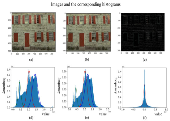
Figure 1. Images and the corresponding histograms: (a) original; (b) reconstruction; (c) residual; (d) original histogram; (e) reconstruction histogram; and (f) residual histogram.

For this reason, another specific learning branch is designed to learn the residual information so that the network can accumulate more details for reconstruction.

1.3.2. Side Information

Few additional coded messages can improve the compression efficiency and quality. For example, block partition messages are often coded and sent to the decoder as side information in traditional JPEG [1], JPEG2000 [2], and H.265 [16] codecs. Ballé et al. [6] and Lee et al. [17] sent standard deviations $\widehat{\sigma }$ with a hyperprior as side information to the latent representations. Agustsson et al. [4] sent additional image semantic information to the generator for better visual quality. Here, compressing the residual with another few bits as side information is adopted to reconstruct the original image.

1.4. Contributions and Paper Organizations

In this paper, the residual learning method is firstly proposed to individually compress the low- and high-frequency information. It reduces not only the difficulty of training model but also the complexity of generating full resolution image distribution. Secondly, it specifically explains and demonstrates that the essence of DL-based image compression is the process of residual learning. Moreover, this paper fully taps the potential of three-level residual learning and improves some existing technical methods in image compression.

The rest of this paper is organized as follows. In Section 2, the proposed framework and the details of each module are illustrated. Section 3 describes some experimental results to demonstrate the effectiveness of all modules. Comparison results with traditional and DL-based codecs are shown. Furthermore, ablation studies are also presented. Section 4 concludes this paper.

2. Proposed Framework

2.1. Overview of the Proposed Framework

The proposed image compression framework is composed of two parts: one is for the main information compression, and the other is for the residual information compression. They both contain convolutional encoder, channel residual quantizer, and convolutional decoder. Figure 2 shows the proposed framework.

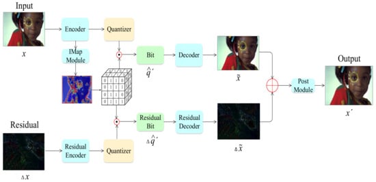
Figure 2. Proposed image compression framework. Note that, for better visualization, the salient region of the residual image was cropped.

From the encoder side, a vector of image intensities x is transformed into latent representation space y, quantized to $\widehat{q}$, multiplied by importance map b to $\widehat{q^{\prime }}$, and then sent to the decoder for reconstruction $\tilde{x}$. Then, the residual $\Delta x(\Delta x=x-\tilde{x}$) is successively transformed to $\Delta y$ by residual encoder, to $\Delta \widehat{q}$ by quantizer, and to $\Delta \widehat{q^{\prime }}$ by multiplying the same importance map b. Finally, residual decoder transforms $\Delta \widehat{q^{\prime }}$ to $\Delta \tilde{x}$ for residual reconstruction. The reconstructed image $x^{\prime }$ is the accumulated outputs of the decoder and residual decoder, x’ = $\tilde{x}$ + $\Delta \tilde{x}$. The coded bit streams are consisted of all quantized bits, q = $\widehat{q^{\prime }}$ + $\Delta \widehat{q^{\prime }}$.

For the encoder, the input image is scaled to $\frac{1}{2^M}·\frac{1}{2^M}$ through M residual blocks with convolutional stride 2 instead of MaxPooling layers. Simple and effective group normalization (GN) was adopted instead of generalized divisive normalization (GDN) mentioned in [6,18]. Before quantization, the channel number is up-sampled to $N_{out}$. On the decoder side, another channel down-sampling and pixel up-scaling operations are taken to reconstruct the image.

2.2. Residual Structure

In the proposed compression framework, both the encoder and decoder are fully convolutional structure regardless of the input image size. The residual blocks are the basic components of the network as shown in Figure 3, which is derived from ResNet architecture firstly proposed for image recognition [19].

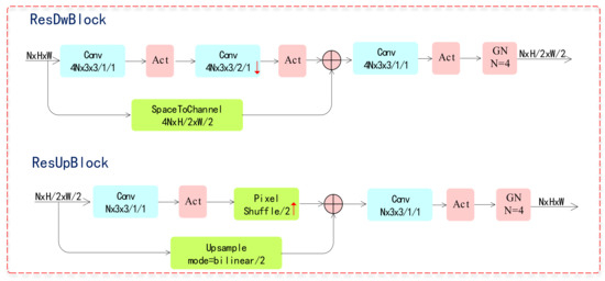
Figure 3. ResDwBlock and ResUpBlock.

2.3. Encoder and Decoder

The encoder consists of four residual blocks with stride 2 for down-sampling. Batch normalization was found to have no beneficial effect and Ballé et al. [18] proved GDN was a good choice. However, group normalization (GN) [20] is simple and also a better choice from the experiments. It is more suitable for local divisive normalization and training large models which require small batches constrained by memory consumption. Moreover, the shortcut structure is introduced to feature fusion and extraction, which transmits more useful information to the following concatenate layer. The decoder also consists of four residual blocks with PixelShuffle layers for up-sampling. The activation function is leakyReLU. The details of the architecture are shown in Figure 4.

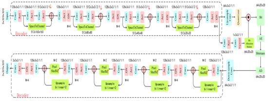
Figure 4. Illustration of the encoder and decoder. The blue box represents residual blocks for down-sampling or up-sampling, convolutional parameters are denoted as filter × kernel height × kernel width/stride/padding, the pink box represents group normalization (GN), activation function (Act), the yellow box is quantizer, the green box represents special operation module, and AE and AD represent arithmetic encoder and arithmetic decoder, respectively.

2.4. Channel Residual Quantization

Quantization is the main part of compression task, which not only compresses data but also introduces errors and noises. Binary representation is an important mean of quantization. A binary bottleneck helps force the network to discard more redundant bit patterns comparing to standard round function or floating-point representation. This paper follows Raiko et al. [21] and Toderici et al. [14] by quantizing the input value $x\in (-1,1)$ to the set $\left\{-1,1\right\}$ for each value. Assuming that $b\left(x\right)\in \left\{-1,1\right\}$ and $x\in (-1,1)$, it can be defined as:

$$b\left(x\right)=x+\epsilon \in \left\{-1,1\right\}$$

(3)

$$\epsilon \sim \left\{\begin{array}{c}-x+1\hspace{1em}with probability\hspace{1em}\frac{1+x}{2}\\ -x-1\hspace{1em}with probability\hspace{1em}\frac{1-x}{2}\end{array}\right.$$

(4)

where $\epsilon$ denotes the quantization noise. For the backward propagation, the derivative of the expectation $\mathbb{E}$ [$b\left(x\right)$] = x, for x$\in (-1,1)$, is used. Therefore, the gradient back propagated through $b\left(x\right)$ is 1. Once the networks are trained, $b\left(x\right)$ is replaced by $b^{inf}$ defined as:

$$b^{inf}\left(x\right)=\left\{\begin{array}{ccc}-1& if& x<0\\ +1& & otherwise\end{array}\right.$$

(5)

As analyzed in Section 1.2, deep channel residual learning method can be used to eliminate the errors between channels to some extent. Therefore, combining the two technologies, a denoising quantization method is employed.

2.5. Improved Importance Map Method for Rate Control

Importance map method for rate control was firstly proposed by Li et al. [7]. Instead of rounding and entropy, they defined rate loss on importance map and adopted a simple binarization for quantization. This method for rate control is content-weighted and benefit to improve visual quality. Here, the part of the architecture in [7] and some novel technologies (e.g., binarization with probability depicted in Section 2.4 and smooth bit allocation with sigmoid function) are adopted. The process is shown in Figure 4.

Intermediate feature maps are utilized to yield content-weighted importance map $p\left(x\right)$. The importance map has only one channel, with the same size as the encoder and the range of (0,1). The value of the map determines the amount of bit allocation and the compression level. A mask $b\left(x\right)$ from $p\left(x\right)$ with the same size as $\widehat{q}$ is generated. The final quantized bit $\widehat{q^{\prime }}$ = $b\left(x\right)\odot$$\widehat{q}$.

Assuming that $1\times h\times w$ is the size of $p\left(x\right)$, n is the up-sampling filter, so the size of the mask is $n\times h\times w$ and the size of the $\widehat{q}$ is $n\times h\times w$. Here, a recurrent bit allocation method was adopted. Given the bit allocation step s, the bit allocation amount in every step and channel direction is $m=\frac{n}{s}$. Assuming that a value is $p_{ij}\left(x\right)$ in $p\left(x\right)$ and the $b\left(p_{ij}\right)$ is the mask value in this step, the allocation method is defined as follows:

$$b\left(p_{ij}\right)\left(x\right)=\left\{\begin{array}{cccc}1& if& (p_{ij}-\frac{i}{s})>0,& i=0,1,\dots ,s\\ 0& & otherwise\hfill & \end{array}\right.$$

(6)

The calculation formula is:

$$b\left(p_{ij}\right)=\frac{1}{2}\times (sign(2\times sigmoid(k\times (p_{ij}-\frac{i}{s}))-1)+1)$$

(7)

where k is a constant, and $i\in \left\{0,1,\dots ,s\right\}$, the size of $b\left(p_{ij}\right)$ is $m\times h\times w$. When the sth step is completed, a mask $b\left(x\right)$ with the size of $n\times h\times w$ is obtained.

The quantization in this stage follows the method depicted in Section 2.4.

2.6. Training Strategy

2.6.1. Loss Function

Generally, jointly optimizing the rate loss and distortion loss is necessary. A trade-off parameter $\lambda$ is used to balance compression rate and distortion. Moreover, another residual distortion loss $D(\Delta x,\Delta \tilde{x})$ is applied. Therefore, the objective function is defined as follows:

$$\mathcal{L}=\sum _{}\left\{{\mathcal{L}}_{D_1}(x,\tilde{x})+\gamma {\mathcal{L}}_{D_2}(\Delta x,\Delta \tilde{x})+\lambda {\mathcal{L}}_R\left(x\right)\right\}$$

(8)

Distortion Loss. As mentioned above, distortion loss is to evaluate the difference between the original image and reconstruction image. Mean square error (MSE), mean absolute error (MAE), or perceptual space loss (MS-SSIM ) is used to define it. In this paper, the distortion is assessed by MSE loss. Besides, another residual loss is added to obtain better visual effect. The total distortion is defined as follows:

$${\mathcal{L}}_D=\sum _{}\left\{{∥x-\tilde{x}∥}^2+\gamma {∥\Delta x-\Delta \tilde{x}∥}^2\right\}$$

(9)

Rate Loss. Importance map is a substitution of entropy estimation. Proper optimization of the bit allocation through the importance map is a good choice to minimize the entropy of the coded bits. Compared to the monotonous region, the region of rich texture gets more coded bits. The optimal goal is to encode the most abundant information with the fewest bits. Therefore, the rate loss can be defined as follows:

$${\mathcal{L}}_R=\frac{1}{M}\sum _{i,j}^m{p}_{ij}\left(x\right)$$

(10)

2.6.2. Optimization Function and Training Details

ADAM optimizer [22] with an initial learning rate 2$\times {10}^{-4}$ is employed. Multi-step learning rate schedule is applied and the decay factor is 0.5. The activation function is leakyReLU. The training hyper-parameters, such as the iteration of residual learning r, the bit allocation step s, the residual blocks’ channel $n_f$, and the up-sampling filter $N_{out}$, are adjustable. In this paper, r = 1, 3; s = 8; $n_f$ = 32, 64, 128; and $N_{out}$ = 32, 64, 128, are set, respectively. In the training process, first the focus is on optimization on the distortion loss, and then it transfers to optimizing the rate loss. Note that increasing the training parameter value can improve the index, but it would also increase the cost and difficulty of training.

3. Experiments

3.1. Experimental Setup

The results reported in this paper were trained on the dataset from Challenge on Learned Image Compression (CLIC). To improve performance, extra images from Flickr2K and DIV2K datasets were added to the training set at the cost of longer training time. The high-quality images were randomly cropped to 320 × 320 pixels and saved as lossless PNGs, with about 100,000 patches in total. The CLIC validation dataset and Kodak PhotoCD image dataset were used to evaluate our models. The compression rate is defined by the bits per pixel (BPP) as follows:

$$BPP=\frac{N_{out}+\Delta N_{out}}{2^M·2^M}·\mathbb{E}\left(b\left(p_{ij}\right)\right)$$

(11)

where $N_{out}$ and $\Delta N_{out}$ are the up-sampling channels, M is the down-sampling number, and $\mathbb{E}\left(b\left(p_{ij}\right)\right)$ is the mean BPP ratio in importance map. The image distortion was evaluated by PSNR and MS-SSIM. Some experiments were finished with the parameters $\lambda$ = 5$\times {10}^{-3}$, 1 $\times {10}^{-2}$, 5$\times {10}^{-2}$, and $N_{out}$ = 32, 64, 128, $M=4$, corresponding to BPP approximately in the range of (0.1,0.5).

In the following, the results of both quantitative metrics and visual quality evaluation are presented, and some ablation studies are shown.

3.2. Experimental Results

3.2.1. Quantitative Evaluation

All trained models were evaluated on the publicly available Kodak dataset (Eastman Kodak, 1993) [23], an uncompressed set of images commonly used to evaluate image compression methods. Image distortion were optimized for MSE and summarized rate-distortion curves are shown in Figure 5. For quantitative evaluation, the test results with JPEG [1], JPEG2000 [2], and the DL-based previous methods such as Theis et al. (2017) [10], Li et al. (2017) [7], and Ballé et al. (2018) [6] were compared.

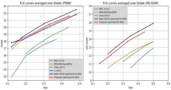
Figure 5. Rate–distortion curves of the proposed method and competitive approaches over the Kodak dataset. The measures are the PSNR and the MS-SSIM value as a function of BPP. Note that the PSNR’s formula is 10$\times lo{g}_{10}\frac{{255}^2}{MSE}$, and MS-SSIM values are converted into decibels for better visualization ($-10\times lo{g}_{10}(1-MSSSIM)$).

In this paper, the distortion is only assessed by mean square error (MSE) loss. Thus, the results shown in Figure 5 are under MSE optimization.Although our approach cannot achieve the state-of-the-art results, the proposed approach outperforms JPEG, JPEG2000, and Theis et al. [10] in PSNR and MS-SSIM index at low BPP. In this paper, the low bit range is less than 0.5 BPP. The corresponding compression ratio is more than 48 times. When the BPP is set 0.1, the corresponding compression ratio is 240 times. It is worth mentioning that the proposed framework performs better at low bits. At low bits, the compression rate is higher, and more residual information is discarded. Thus, the specific residual learning network is more suitable to learn representative residual features.

3.2.2. Visual Quality Evaluation

Furthermore, visual quality evaluation is arranged to demonstrate the effectiveness of the deep residual learning algorithm by comparing it with JPEG, JPEG2000, and Ballé (2018). Figure 6, Figure 7 and Figure 8 clearly show that artifacts, blurring, and blocking are obvious the in traditional image compression algorithms, e.g., JPEG and JPEG2000. Although Ballé’s (2018) PSNR is higher than the proposed model, the visual quality is not good enough. The proposed framework is good at eliminating blocking effect and smoothing the blurs.

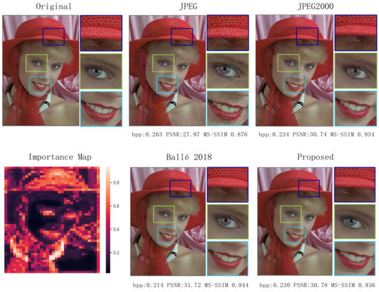
Figure 6. Visual quality evaluation of the specific image named kodim04 in Kodak dataset with different approaches.

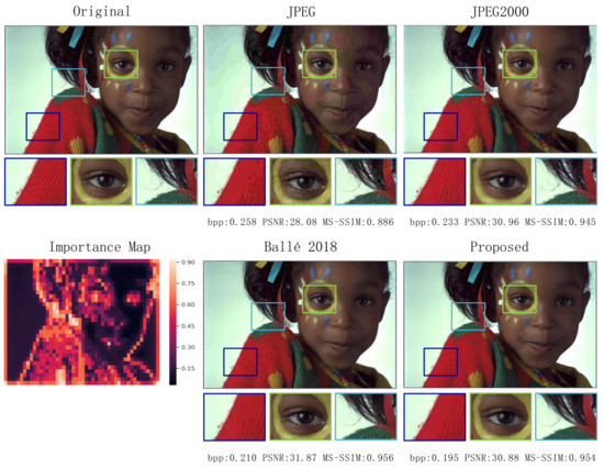
Figure 7. Visual quality evaluation of the specific image named kodim15 in Kodak dataset with different approaches.

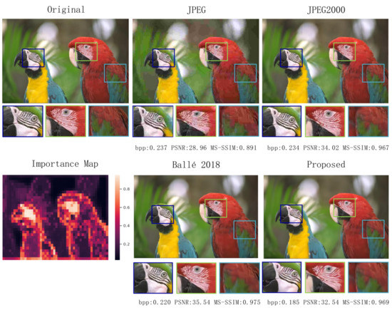
Figure 8. Visual quality evaluation of the specific image named kodim23 in Kodak dataset with different approaches.

3.3. Ablation Studies

To train a better image compression model, many ablation experiments were implemented. The results of ablation study are shown below, such as importance map for rate control, channel residual learning, global residual learning, etc.

3.3.1. Importance Map

To assess the role of importance map, the training process of the baseline model without importance map was compared to the model with importance map at about 0.47 BPP. For the sake of fairness, the sizes of the two models were the same approximately. The details during training phase are shown in Figure 9a. The importance map is used for rate estimation, and improves the performance by about 2 dB. Moreover, the importance map of the specific image named kodim15 in Kodak dataset is shown in Figure 9b. The figure exhibits that the red region represents the value $p_{ij}\left(x\right)$ is large, where more bits are allocated, such as the regions with rich texture and edge.

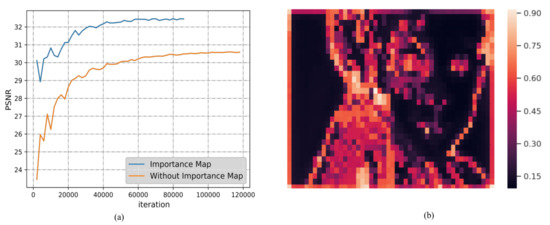
Figure 9. (a) PSNR performance during the training phase and the process of residual learning at about 0.47 BPP; amd (b) importance map of image kodim15 in Kodak dataset.

3.3.2. Channel Residual Learning

As with the above experiments, a baseline model without channel residual learning and another model with channel residual learning were implemented at about 0.47 BPP on CLIC test dataset. As shown in Figure 10, the PSNR is also improved about 0.4 dB. Therefore, channel direction residual learning may eliminate the noise, as described in Section 1.2.

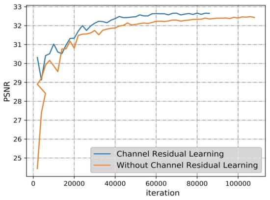
Figure 10. Results of ablation experiments about channel residual quantization.

3.3.3. Global Residual Learning

In Figure 5, the performance of the proposed framework is better than the method proposed by Li et al. [7] in PSNR. The most improved performance is the result of global residual learning. The specific residual learning branch is designed to encode the residual information. As the side information, it is added to the quantized bits. The details of the global residual learning process are shown in Figure 11.

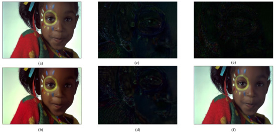
Figure 11. Process of global residual learning: (a) original x; (b) main information $\tilde{x}$; (c) residual $\Delta x$; (d) reconstructed residual $\Delta \tilde{x}$; (e) remained residual $\Delta x^{\prime }$; and (f) reconstruction $x^{\prime }=\tilde{x}+\Delta \tilde{x}$. Note that for better visualization, salient region of the residual image was cropped.

3.3.4. Other Experiments

Increasing the iteration of residual learning can also improve the performance at the cost of training time and training difficulty. Another model with residual block channels $n_f$ = 128, up-sampling channels $N_{out}$ = 64, and iteration of residual learning r = 3 was trained. Although the PSNR improved by about 0.5 dB, the model size increased by about two times.

To further improve performance and eliminate artifacts and blurs, a post-processing module similar to [24] is adopted to fine-tune on the trained model. Because the result of residual learning is added to the reconstruction image in this paper, the post-processing module can better integrate the information of both.

4. Conclusions

In this paper, a deep residual learning based image compression framework is proposed. Learning the residual distribution is easier compared to learning the full resolution information through the analysis of residual distribution. The high- and the -frequency components are separated to compress individually. At the same time, improved importance map methods are introduced to realize better bit allocation. Experimental results show that residual learning mechanism can improve the compression performance by focusing on key residual information. In the future, the entropy module will be introduced for rate estimation comparison and training models with higher BPP.

References

- Wallace, G. The JPEG still picture compression standard. Commun. ACM 1991, 34, 30–44. [Google Scholar] [CrossRef]
- Rabbani, M. JPEG2000: Image Compression Fundamentals, Standards and Practice. J. Electron. Imaging 2002, 11. [Google Scholar] [CrossRef]
- Goyal, V.K. Theoretical foundations of transform coding. IEEE Signal Process. Mag. 2001, 18, 9–21. [Google Scholar] [CrossRef]
- Agustsson, E.; Tschannen, M.; Mentzer, F.; Timofte, R.; Gool, L.V. Generative Adversarial Networks for Extreme Learned Image Compression. arXiv 2018, arXiv:1804.02958. [Google Scholar]
- Choi, Y.; El-Khamy, M.; Lee, J. Variable Rate Deep Image Compression With a Conditional Autoencoder. In Proceedings of the IEEE International Conference on Computer Vision (ICCV), Seoul, Korea, October 2019. [Google Scholar]
- Ballé, J.; Minnen, D.; Singh, S.; Hwang, S.J.; Johnston, N. Variational image compression with a scale hyperprior. arXiv 2018, arXiv:1802.01436. [Google Scholar]
- Li, M.; Zuo, W.; Gu, S.; Zhao, D.; Zhang, D. Learning Convolutional Networks for Content-weighted Compression. arXiv 2017, arXiv:1703.10553v2. [Google Scholar]
- Mentzer, F.; Agustsson, E.; Tschannen, M.; Timofte, R.; Van Gool, L. Conditional Probability Models for Deep Image Compression. arXiv 2018, arXiv:1801.04260. [Google Scholar]
- Rippel, O.; Bourdev, L. Real-Time Adaptive Image Compression. arXiv 2017, arXiv:1705.05823. [Google Scholar]
- Theis, L.; Shi, W.; Cunningham, A.; Huszár, F. Lossy Image Compression with Compressive Autoencoders. arXiv 2017, arXiv:1703.00395. [Google Scholar]
- Web. WebP Image Format. Available online: https://developers.google.com/speed/webp (accessed on 9 June 2020).
- Bellard, F. BPG Image Format. Available online: https://bellard.org/bpg/ (accessed on 9 June 2020).
- Wang, Z.; Simoncelli, E.P.; Bovik, A.C. Multiscale structural similarity for image quality assessment. In Proceedings of the Thrity-Seventh Asilomar Conference on Signals, Systems Computers, Pacific Grove, CA, USA, 9–12 November 2003; Volume 2, pp. 1398–1402. [Google Scholar] [CrossRef]
- Toderici, G.; O’Malley, S.M.; Hwang, S.J.; Vincent, D.; Minnen, D.; Baluja, S.; Covell, M.; Sukthankar, R. Variable Rate Image Compression with Recurrent Neural Networks. arXiv 2015, arXiv:1511.06085. [Google Scholar]
- Johnston, N.; Vincent, D.; Minnen, D.; Covell, M.; Singh, S.; Chinen, T.T.; Hwang, S.J.; Shor, J.; Toderici, G. Improved Lossy Image Compression with Priming and Spatially Adaptive Bit Rates for Recurrent Networks. arXiv 2017, arXiv:1703.10114. [Google Scholar]
- Sullivan, G.J.; Ohm, J.; Han, W.; Wiegand, T. Overview of the High Efficiency Video Coding (HEVC) Standard. IEEE Trans. Circuits Syst. Video Technol. 2012, 22, 1649–1668. [Google Scholar] [CrossRef]
- Lee, J.; Cho, S.; Beack, S.K. Context-adaptive Entropy Model for End-to-end Optimized Image Compression. arXiv 2018, arXiv:1809.10452,. [Google Scholar]
- Ballé, J.; Laparra, V.; Simoncelli, E.P. End-to-end Optimized Image Compression. arXiv 2016, arXiv:1611.01704. [Google Scholar]
- He, K.; Zhang, X.; Ren, S.; Sun, J. Deep Residual Learning for Image Recognition. arXiv 2015, arXiv:1512.03385. [Google Scholar]
- Wu, Y.; He, K. Group Normalization. arXiv 2018, arXiv:1803.08494. [Google Scholar]
- Raiko, T.; Berglund, M.; Alain, G.; Dinh, L. Techniques for Learning Binary Stochastic Feedforward Neural Networks. arXiv 2014, arXiv:1406.2989. [Google Scholar]
- Kingma, D.P.; Ba, J. Adam: A Method for Stochastic Optimization. arXiv 2014, arXiv:1412.6980. [Google Scholar]
- Eastman Kodak. Kodak Lossless True Color Image Suite (Photocd pcd0992). 1993. Available online: http://r0k.us/graphics/kodak/ (accessed on 9 June 2020).
- Zhou, L.; Cai, C.; Gao, Y.; Su, S.; Wu, J. Variational Autoencoder for Low Bit-rate Image Compression. In Proceedings of the IEEE Conference on Computer Vision and Pattern Recognition (CVPR) Workshops, Austin, TX, USA, June 2018. [Google Scholar]
© 2020 by the authors. Licensee MDPI, Basel, Switzerland. This article is an open access article distributed under the terms and conditions of the Creative Commons Attribution (CC BY) license (http://creativecommons.org/licenses/by/4.0/).