Weak Signal Detection Method Based on the Coupled Lorenz System and Its Application in Rolling Bearing Fault Diagnosis

Abstract

Rolling bearings are widely used in rotating machinery. Their fault feature signals are often submerged in strong noise and are difficult to identify. This paper presents a new method of bearing fault diagnosis that combines the coupled Lorenz system and power spectrum technology. The process is achieved in the following three steps. First, a synchronization system based on the Lorenz system is constructed using the driving-response method. Second, when the tested signal is connected to the driving end, the synchronization error between the two sub-chaotic systems is obtained. Finally, the power spectrum density of the synchronization error is calculated and compared with the corresponding fault characteristic frequency. The coupled Lorenz system makes full use of the noise immunity and nonlinear amplification of the chaotic system. The detection characteristics and feasibility of the new method are verified by simulation and actual measured vibration data. The result shows that the noise reduction effect of the coupled Lorenz system is obvious. This method can improve the signal-to-noise ratio of the tested signal and provide a new way to perform fault diagnosis of rolling bearings.

1. Introduction

A rolling bearing is a precision mechanical element that is widely used in many mechanical devices, and it is a vulnerable component. In many practical applications, it is necessary to detect the running status of a rolling bearing online to provide a guarantee for the safe and stable operation of mechanical equipment [1,2]. There are many failure modes of rolling bearings, including pitting, cracking, stripping, scraping and so on. When the bearing runs to these fault parts, it will produce vibration and shock. However, due to the short impact time and scattered energy, in the early stage of the fault, the corresponding fault characteristic signal is very weak and is covered by a large amount of machine running noise, so it is difficult to distinguish the fault signal by the traditional signal processing method. Therefore, it is necessary to preprocess the measured vibration signal to improve its signal-to-noise ratio (SNR) before detecting the fault characteristic signal.

The weak signal detection method based on chaotic systems makes use of the characteristics of chaotic systems, such as sensitivity to the initial value, immunity to noise and nonlinear amplification, to achieve signal detection. Many studies have found that signal detection methods based on chaotic systems can detect a signal with SNR lower than $-30$ dB [3]. This kind of method is completely different from the traditional detection technology. Furthermore, this approach is one of the important research directions of chaos theory that can be applied in practical engineering and thus has broad application prospects.

Since the 1990s, many scholars have studied the signal detection method based on chaotic systems and have been devoted to the expansion and supplement of weak signal detection technology [4]. These studies mainly focus on the following three aspects. The first aspect is the research on the signal detection mechanism and the operation state recognition method of the chaotic system. Representative studies are as follows. S. Zhang used chaotic oscillator as a detector for BPSK signals in very low signal-to-noise ratio (SNR) conditions in Ref. [5]. X. Xiang proposed a method based on the chaotic oscillator for weak signal detection using information fusion technology in Ref. [6]. J. Faber found the analytic response function of a non-isochronous Hopf oscillator to a step stimulus in Ref. [7]. V. Rashtchi proposed that the transformation of state can be judged by calculating the autocorrelation coefficient of phase space trajectories, and performed a comparison with the maximum Lyapunov exponent method in Ref. [8]. However, these methods are based on the assumption that the frequency of the weak signal is known, which greatly restricts the application of these methods.

The second aspect is the research on the measurement method of the weak signal with unknown frequency. To solve this problem, C. Cong studied the intermittent chaos phenomenon of the Duffing oscillator system and proposed a new method for detecting various parameters of the periodic signal in Ref. [9]. G. Li proposed a new method of frequency estimation by searching the maximum value of the phase space trajectory variance based on a genetic algorithm in Ref. [10]. Zhao presented a method of detecting the signal frequency by the intermittent chaos in Ref. [11]. However, the structure and parameter settings of chaotic system models used in these studies are very complex.

The third aspect is the research on the application and implementation of chaotic detection systems. The representative studies are as follows. V. Rashtchi tried to use the Duffing oscillator to detect eccentric faults of motors under different load conditions in Ref. [12]. Bai proposed an enhanced differential chaos shift keying (DCSK), based on a first-order hybrid chaotic system, for a high-reliability underwater acoustic communication system in Ref. [13].

Obviously, the above studies are focused on the problems of detecting weak signals using a single chaotic system. These methods must strictly set up the structural parameters of the chaotic system and accurately judge the running state and the phase space trajectories of the system. That requirement makes them susceptible to many shortcomings, such as a low operating efficiency, a large amount of calculation, a difficult state determination, and a capability of being easily influenced by the change of parameters, and they cannot be applied directly to the noise reduction processing of bearing vibration signals.

The synchronization of two chaotic systems with different initial states is an important characteristic of chaotic systems. Many scholars have put forward some data encryption methods based on this characteristic [14,15]. In addition, some scholars studied the synchronization method of chaotic systems with unknown parameters or different structures [16,17]. These related studies provide a theoretical basis for noise reduction via chaotic synchronization [18,19]. Considering that the synchronization error of two chaotic systems can reflect the change in the input signal, a new method of noise reduction based on the coupled Lorenz system is proposed in this paper and applied to bearing fault diagnosis. Compared with the existing methods, the proposed method improves the real-time performance and adaptability, and has a good denoising effect on the tested vibration signal.

This paper is organized as follows. In Section 2, the noise reduction mechanism and frequency estimation method based on the Lorenz system are discussed. In Section 3, the detection characteristics of the established model and the difference between the traditional chaotic detection method are simulated and analyzed. In Section 4, the feasibility of the new method applied to vibration data processing of a rolling bearing is discussed. This paper ends with some concluding remarks in Section 5.

2. Noise Reduction Mechanism and Frequency Estimation Method Based on the Coupled Lorenz System

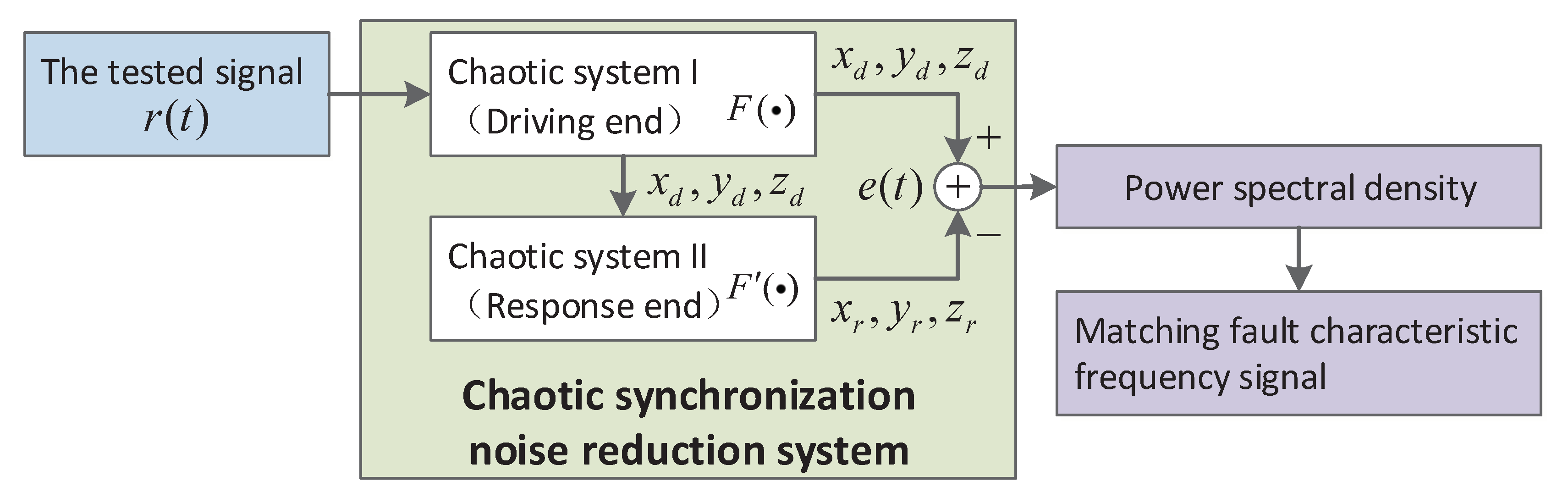
2.1. Theoretical Model and Working Mechanism

In this paper, a new method is used to detect a weak signal submerged in strong background noise; its SNR is usually less than $-20$ dB, and the equation is

$$r\left(t\right)=s\left(t\right)+n\left(t\right),$$

(1)

where $s\left(t\right)$ is a weak sinusoidal signal $Asin(\omega t+\theta )$, $n\left(t\right)$ is the Gaussian white noise whose probability density follows the normal distribution. Its mean value is 0, its variance is ${\sigma }^2$, and its expression is $N(0,{\sigma }^2)$. This kind of signal exists in many fields, including power electronics, rotating machinery, clinical medicine and so on. According to the related theory of signal processing, if each signal with different frequencies in the tested signal can be accurately distinguished, fault diagnosis can be achieved by finding the peak value of the power spectrum density and comparing it with the value of the fault characteristic frequency.

Regarding the above discussions, there are still many limitations in the existing chaotic detection methods that cannot be directly used in fault diagnosis. Therefore, we propose two chaotic systems with the same structure to form a synchronization system to achieve the detection of the fault characteristic signal. The block diagram of the detection system is shown in Figure 1.

In this system, the chaotic system I is used as the driving end and the chaotic system II is used as the response end. The two ends are coupled by the drive-response method.

The diagnostic process is divided into three steps. First, the tested signal is injected into the chaotic system I, which results in the deviation of the state variables of the two chaotic systems. Second, the state variables of the two chaotic systems at the same position are obtained simultaneously, and the synchronization error can be obtained. Finally, the power spectral density of the synchronization error $e\left(t\right)$ is calculated and matched with the fault characteristic frequency to realize the fault diagnosis. This system makes full use of the characteristics of the chaotic system and enhances the periodic signal while restraining the influence of white noise, thus improving the signal-to-noise ratio of the tested signal.

2.2. Selection and Configuration of Chaotic Model

Most of the existing studies on weak signal detection are based on the Duffing oscillator system. This kind of system contains a periodic dynamic force, whose frequency must be consistent with the tested signal, and it runs at the critical point of the state transition. These requirements greatly increase the complexity of the system and such that it cannot be applied to situations where there are several periodic signals with different frequencies or the tested signal with an unknown frequency.

The Lorenz system is a classic three-dimensional chaotic system that was first studied by Edward Lorenz in 1963 [20]. This system has the advantages of a simple structure and easy construction and has chaotic solutions under some parameter values and initial conditions. Therefore, we studied the method of detecting the frequency of weak signal using the Lorenz system. Its mathematical model is as follows:

$$\left\{\begin{array}{c}\frac{dx}{dt}=\sigma (y-x)\hfill \\ \frac{dy}{dt}=x(\rho -z)-y+r\left(t\right).\hfill \\ \frac{dz}{dt}=xy-\beta z\hfill \end{array}\right.$$

(2)

The $r\left(t\right)$ is the test signal, which does not exist in the standard Lorenz system. It changes the model (Equation (2)) into a higher-dimensional dynamical system. We studied the dynamic characteristics of this system by setting its structural parameters ($\sigma =10$, $\beta =2.6$) and obtained the bifurcation diagram of the parameter $\rho$, as shown in Figure 2.

This figure can be divided into five intervals, in which the critical points are $\rho =24$, 150, 169 and 215. Therefore, the running state of the chaotic system goes through the multi-periodic state and chaotic state as the parameter $\rho$ increases. Furthermore, we made the system run in different states by changing the value of $\rho$, and observed the changes in the phase space trajectory with different signal inputs $r\left(t\right)$, as shown in Figure 3.

In Figure 3a, $\rho =20$, and the system runs in a multi-periodic state, while in Figure 3b,c, $\rho =50$, and the system runs in chaotic state. In the above figure, curve a is obtained when $r\left(t\right)=0$, curve b is obtained when $r\left(t\right)=0.001sin\left(t\right)$, curve c is obtained when $r\left(t\right)$ is a white noise with a variance of $0.001$, and curve d is obtained when $r\left(t\right)$ is composed of the above sinusoidal signal and the noise signal.

It can be seen that the four curves almost coincide with each other and are hard to distinguish in Figure 3a. Correspondingly, in Figure 3b,c, curves a and c are almost coincident, and curves b and d are also very close to each other, but there are great differences between the two groups of curves. This figure shows that the phase space trajectory will only swing slightly under the influence of noise, but will produce a substantial offset under the influence of a periodic signal, and the offset value is far greater than the amplitude of the periodic signal when the system is running in a chaotic state. Meanwhile, the values of state variables are bounded, which is conducive to the detection of a weak signal in strong noise. Therefore, we use the chaotic synchronization system based on the Lorenz system to obtain the change value of the phase space trajectory to achieve noise reduction.

2.3. Noise Reduction Model Based on the Coupled Lorenz System

Referring to the principle block diagram in Figure 1, we used the drive-response method to build the noise reduction system based on the Lorenz system [21,22]. The state equation of chaotic system I is

$$\left\{\begin{array}{c}\frac{d{x}_d}{dt}=\sigma (y_d-x_d)\hfill \\ \frac{d{y}_d}{dt}=x_d(\rho -z_d)-y_d+r\left(t\right).\hfill \\ \frac{d{z}_d}{dt}=x_d{y}_d-\beta z_d\hfill \end{array}\right.$$

(3)

The state equation of the chaotic system II is

$$\left\{\begin{array}{c}\frac{d{x}_r}{dt}=\sigma (y_d-x_r)\hfill \\ \frac{d{y}_r}{dt}=x_d(\rho -z_d)-y_r.\hfill \\ \frac{d{z}_r}{dt}=x_d{y}_d-\beta z_r\hfill \end{array}\right.$$

(4)

It can be proved that the chaotic system I and II can be synchronized when $\sigma >0$, $\beta >0$ and the input signal $r\left(t\right)=0$.

To prove the above conclusion, we constructed the Lyapunov function, which is

$$V\left(e_x,e_y,e_z\right)=\frac{1}{2}\left(e_x^2+e_y^2+e_z^2,\right).$$

(5)

In this function, the terms $e_x=x_d-x_r$, $e_y=y_d-y_r$, and $e_z=z_d-z_r$. For its derivation, there is

$$\frac{dV\left(e_x,e_y,e_z\right)}{dt}=e_x{e}_x^{\prime }+e_y{e}_y^{\prime }+e_z{e}_z^{\prime }.$$

(6)

Then, combined with Equations (3) and (4) and the condition $r\left(t\right)=0$, the synchronization error system is obtained. The equation is

$$\left\{\begin{array}{c}\frac{d{e}_x}{dt}=-\sigma e_x\hfill \\ \frac{d{e}_y}{dt}=-e_y.\hfill \\ \frac{d{e}_z}{dt}=-\beta e_z\hfill \end{array}\right.$$

(7)

Furthermore, this equation is insert into Equation (6), such that there is

$$\frac{dV\left(e_x,e_y,e_z\right)}{dt}=-\sigma e_x^2-e_y^2-\beta e_z^2.$$

(8)

When $\sigma >0$ and $\beta >0$, there is $\frac{dV\left(e_x,e_y,e_z\right)}{dt}<0$. Thus, referring to the Lyapunov stability theorem [23], the synchronization error system of the above two chaotic systems is uniformly asymptotically stable at the origin. It means that the chaotic system I and II can be synchronized when $\sigma >0$, $\beta >0$ and the input signal $r\left(t\right)=0$.

3. Simulation Analysis and Method Comparison

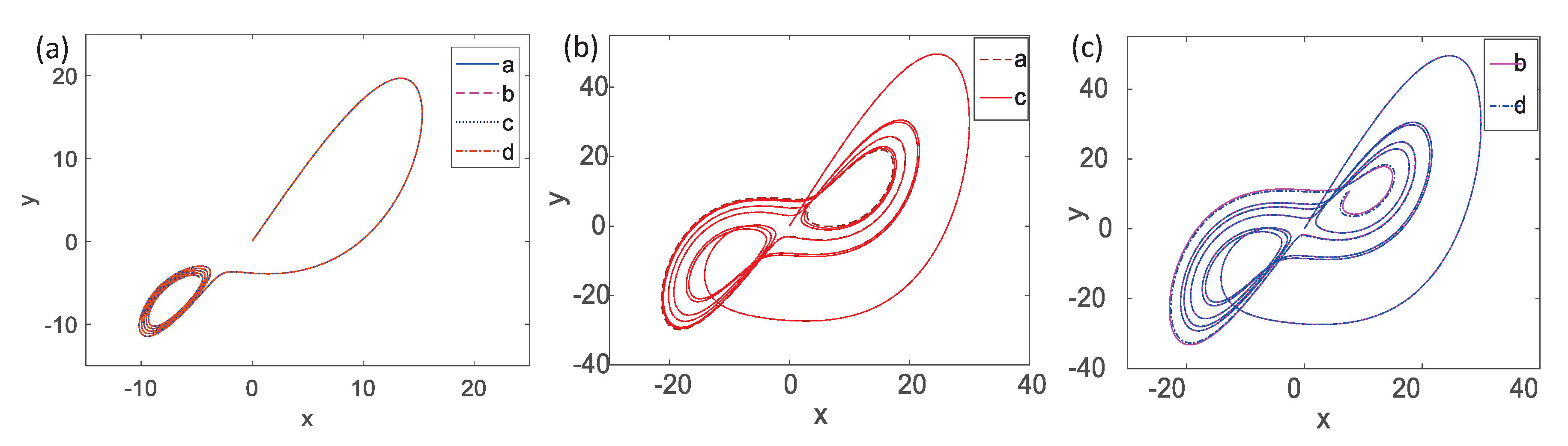
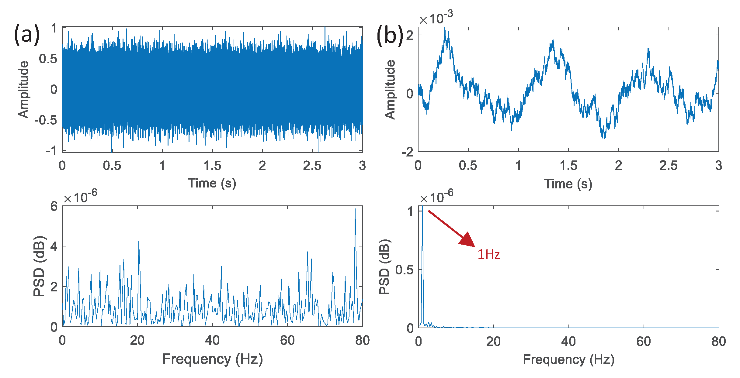
3.1. Simulation Analysis of the Coupled Lorenz System

When the tested signal is input into the coupled Lorenz system as a disturbance term, it will have an impact on the running state of the system, and the phase space trajectory of the two chaotic systems will lose synchronization. The synchronization error $e\left(t\right)$ is the average value of the sum of the corresponding deviations of the three state variables. The equation is as follows.

$$e\left(t\right)=\frac{1}{3}\left(e_x+e_y+e_z\right).$$

(9)

According to the effect of the white noise and the periodic signal on the phase space trajectory, the synchronization error between the two ends $e\left(t\right)$ is mainly influenced by the periodic signal, and the SNR of the synchronization error data will be greatly improved compared with the tested signal.

The structural parameters of the Lorenz system are set to $\sigma =10$, $\beta =2.6$. Referring to Figure 3b, when $\rho =50$, the Lorenz system runs in the chaotic state, which can better identify the periodic signal. Therefore, we configured the chaotic system as the above parameters. To verify the inference proposed above, a sinusoidal signal $0.001sin\left(2\pi t\right)$ and a white noise ($N(0,0.05)$) are superimposed as the tested signal $r\left(t\right)$, and its SNR is

$$SN{R}_{r\left(t\right)}=10lg\left(P_{s\left(t\right)}/P_{n\left(t\right)}\right)=-50dB.$$

(10)

The time domain waveform and power spectral density of the tested signal and the synchronization error are shown in Figure 4.

It can be seen that the weak sinusoidal signal has been masked in the noise in Figure 4a. It is difficult to directly distinguish in the frequency domain. In Figure 4b, a considerable amount of noise is filtered out in the synchronization error, and its SNR is greatly improved. By finding the peak value of the power spectral density, the frequency of the sinusoidal signal obtained from this figure is 1 Hz, which is consistent with the actual value. The simulation result shows that the new coupled Lorenz system has a good noise reduction function.

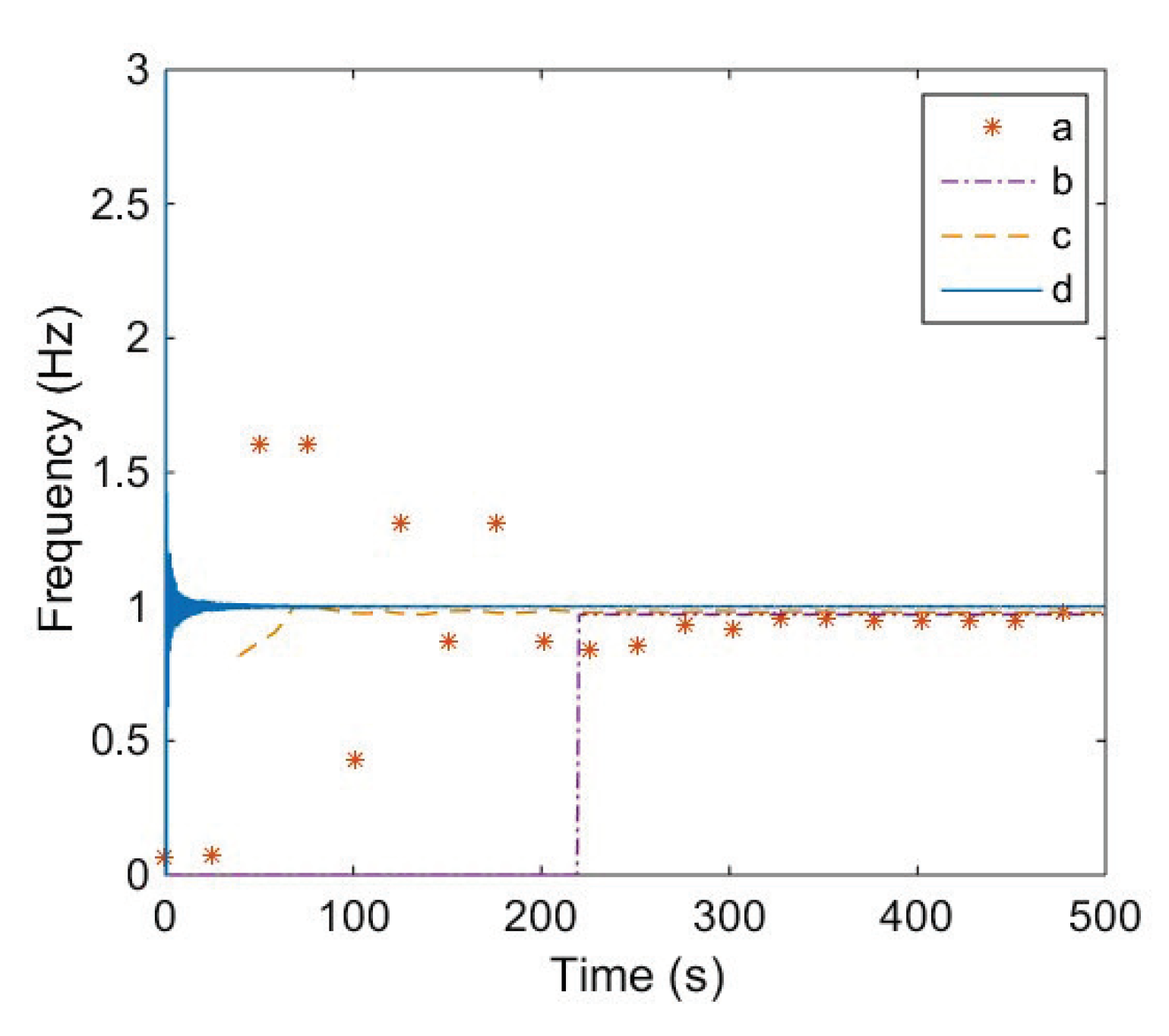
3.2. Effective Range of Frequency Detection

For practical application, it is necessary to study the effective detection range of the coupled Lorenz system, including the amplitude and frequency of the tested signal. To this end, we obtained the bifurcation diagram of the sinusoidal signal A and the SNR curve with frequency variation using the same model and parameter settings used in Section 3.1, as shown in Figure 5.

In Figure 5a, it can be seen that the running state of the Lorenz system varies between the multi-periodic state and the chaotic state with as the amplitude of the sinusoidal signal increases. The amplitude of the sinusoidal signal $A=45$ is the critical point of the state transition of the chaotic system. Therefore, considering that only when the Lorenz system is running in the chaotic state can it have filtering characteristics, the detection range of the amplitude is from 0 to 45 when the Lorenz system uses the above parameters.

In Figure 5b, the curve is the corresponding SNR value of the synchronization error obtained by changing the frequency of the sine signal submerged in the tested signal. It can be seen that the SNR of the synchronization error is greatly improved by the chaotic system compared with that of the tested signal. The improvement effect is greater than 30 dB in the range of 0–200 Hz. This means that the accuracy of the traditional method can be greatly improve when the data preprocessed by this method is used for analysis.

3.3. Comparison with Existing Chaotic Detection Methods

The new method proposed in this paper is not consistent with the existing chaotic detection methods in principle and the implementation mode. To reflect the difference between these methods, the new method is compared with the methods used in the Refs. [8,10,11,18] in some aspects, as shown in

Table 1. Detection methods comparison.

Type	Mode	Measurable Range	Measurable Parameters	Time
Method I [8]	Duffing oscillator	$S_1$	A	$T_1$
Method II [10]	Duffing oscillator array	$S_2$	$\omega$	$T_2$
Method III [11]	Duffing oscillator array	$S_3$	$\omega$	$T_3$
Method IV [18]	Chua’s circuit	$S_4$	$\omega$	$T_4$
Proposed method	Lorenz system	S	$\omega$	T

.

By comparing the principles of these detection methods, it can be seen that method I is based on a single Duffing system to achieve amplitude detection of the weak signal with specific frequency. The measurable range $S_1$ depends on the critical point chosen and the interval width to keep the operation state; it can only be used for amplitude detection, and the time length for determining the system running state is related to the frequency and phase of the tested signal. The detection time $T_1$ is not less than $6/\omega$ to prevent misjudgement, in which $\omega$ is the frequency value of the tested signal.

Method II is based on the optimization algorithm, and method III is based on the intermittent chaos. The measurable range $S_2$ and $S_3$ is related to the number of oscillators used. The larger the range is, the more the number of oscillators needed, which will greatly increase the complexity of the system. Both methods can achieve frequency measurement and need to judge the running state of the system, which affects the detection efficiency. In method II, the detection time $T_2$ is equal to $m\times T_1$, and m is the iteration times of the optimization algorithm. In method III, the determination of intermittent chaos is more difficult, and the detection time $T_3$ is approximately (5∼6) $T_1$.

Method IV is based on two chaotic synchronization systems; its measurable range is affected by the divergent state of the Chua’s circuit, and the amplitude of the tested signal cannot be greater than 0.147. Its detection time is limited by the adaptive controller and is usually set to $T_4=(4-5)/\omega$.

Correspondingly, the simulation results show that the measurable range of the new method S is much larger than that of other methods $S\gg S_2,S_3,S_4$. When the detection time $T=3/\omega$, the new method achieves a good noise reduction effect. Its detection efficiency is much higher than other methods $T\approx T_4\gg T_3\gg T_2\approx m\times T_1$.

To compare the detection efficiency and accuracy of the above methods, we used these methods to estimate the frequency of the same test signal ($r\left(t\right)$ in Section 3.1), and the results obtained are shown in Figure 6.

In Figure 6, there are four curves, which represent the estimated frequencies obtained by the different methods. Curve a obtained by method II is composed of a set of discrete points, which are the optimal particles after each iteration of the genetic algorithm. The final estimated value is 0.965 Hz, and the time required is more than 470 s. Curve b obtained by method III is stable when the time is more than 219 s and the detection value is 0.97 Hz. Curve c obtained by method IV changes around the actual value 1 Hz after 60 s, and fluctuation range is gradually decreasing. When the time reaches 150 s the estimated value is 0.98 Hz. Curve d obtained by proposed method estimates that the frequency value of the test signal is 1.02 Hz at 15 s, then fluctuates between 9.995 Hz and 1.005 Hz. The simulation results show that the new method is superior to the existing methods in detection efficiency and accuracy.

4. Application of the New Method in Fault Diagnosis of Rolling Bearing

4.1. Fault Mechanism and Characteristic Frequency

When the rolling bearing is running, the main sources of vibration excitation include the following items: the error caused by installation and manufacture, the change of the axle center caused by the working load, the deformation of the contact position caused by a heavy load, and so on. These vibrations generate considerable noise, making it difficult to distinguish the vibration impact produced by the damaged part through the load area from them.

The frequency of the impact is the corresponding fault characteristic frequency, which can be calculated from the rotation speed of the shaft, the size of the bearing and the location of the damage point. The key parameters are as follows: z is the number of rolling elements, d is the diameter of the rolling body, D is the diameter of bearing, $\alpha$ is the contact angle, $f_r$ is the frequency of the inner ring, and $f_a$ is the frequency of the outer ring. The following is the calculation formula of the fault characteristic frequency in three cases of inner ring damage $f_i$, outer ring damage $f_o$ and rolling element damage $f_b$.

$$f_i=\frac{z}{2}\left|f_a-f_r\right|(1+\frac{d}{D}cos\alpha ).$$

(11)

$$f_o=\frac{z}{2}\left|f_a-f_r\right|(1-\frac{d}{D}cos\alpha ).$$

(12)

$$f_b=\frac{D}{2d}\left|f_a-f_r\right|(1-\frac{d^2}{D^2}co{s}^2\alpha ).$$

(13)

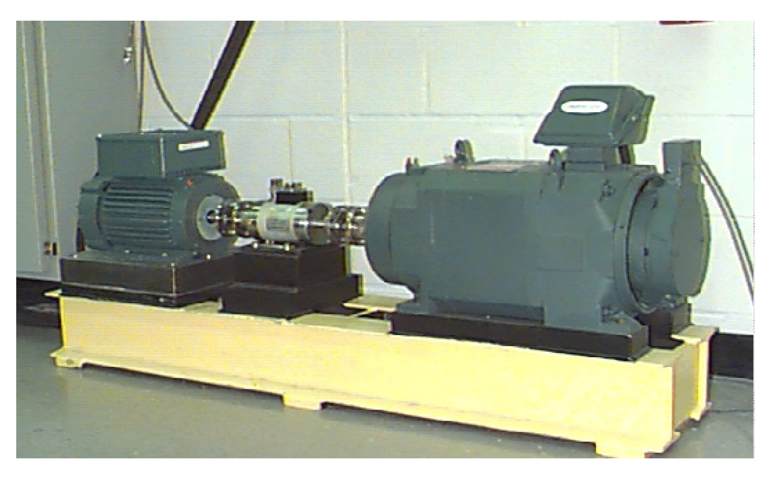
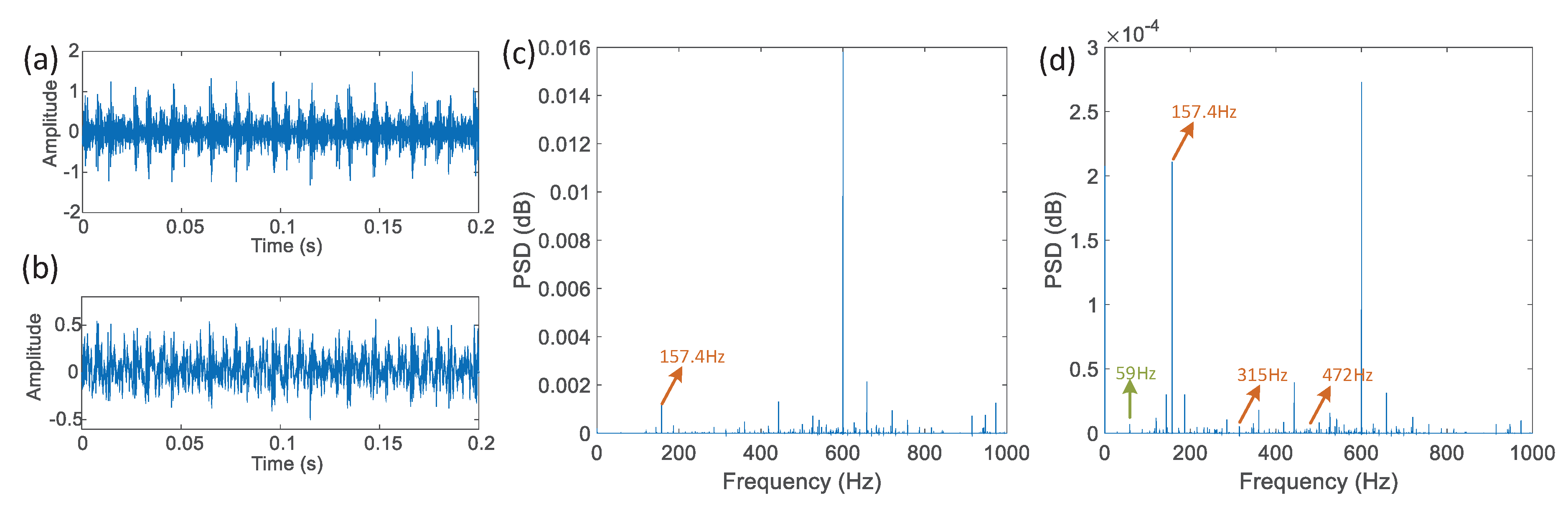
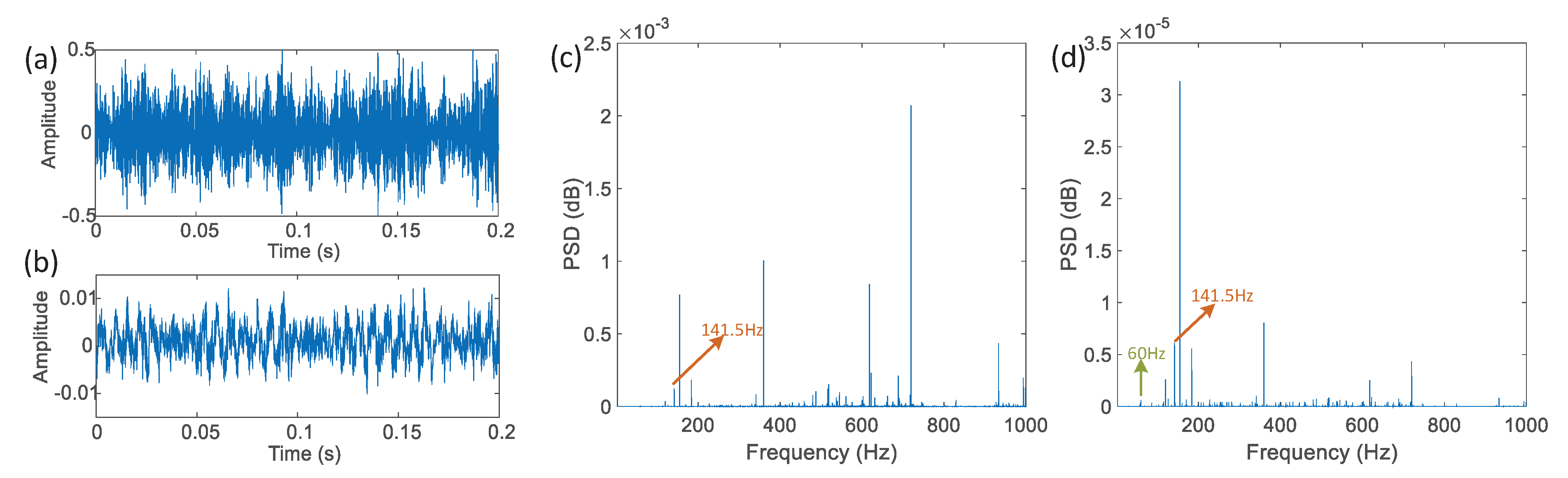
4.2. Experimental Verification

We use the actual measured data to verify the feasibility of the coupled Lorenz system applied to rolling bearing vibration signal processing. These data are measured by the bearing data center of the Case Western Reserve University, and the test platform used is shown in Figure 7.

In this figure, the test stand consists of a 2 hp motor (left), a torque transducer/encoder (center), a dynamometer (right), and control electronics (not shown). The test bearings support the motor shaft. Single point faults were introduced to the test bearings using electro-discharge machining. Vibration data were collected using accelerometers that were attached to the housing with magnetic bases, and the sampling rate is 12,000 S/s. The tested bearing is a 6205-2RS JEM SKF deep groove ball bearing, and its basic parameters are shown in

Table 2. Bearing specification table (inches).

Inside Diameter	Outside Diameter	Thickness	Ball Diameter	Pitch Diameter
0.9843	2.0472	0.5906	0.3126	1.537

.

The number of the rolling element z is 9, and the contact angle $\alpha$ is 0. Referring to Equations (11)–(13), the coefficient relationship between the fault characteristic frequency and the rotation rate can be obtained, when the inner ring, outer ring and rolling element are damaged. These coefficients are shown in

Table 3. Defect frequencies (multiple of running speed in Hz).

Inner Ring	Outer Ring	Rolling Element
5.4152	3.5848	4.7135

.

We take the vibration data of the inner ring with $0.007inch$ of single point damage as the tested signal, and implement it in the coupled Lorenz system established above. Then, the time domain waveform of the vibration signal and the synchronous error and the power spectrum density of these two signals are obtained, as shown in Figure 8.

Figure 8c is directly calculated from the actual vibration signal in Figure 8a, and Figure 8d is calculated from the synchronous error data in Figure 8b. At this time, the motor speed is 1748 rpm, and the double rotation frequency of bearing is 59 Hz. Combined with the coefficients in Table 1, the characteristic frequency of the inner ring fault is 157.7628 Hz. Compared with the subgraphs Figure 8c,d, it is obvious that the double frequency of bearing rotation, the fault feature frequency of the inner ring damage and multiple harmonics of fault frequency are greatly enlarged after the noise reduction, which can be easily identified.

Furthermore, we use the same method and model to process the vibration data of the outer ring with $0.007inch$ of single point damage. The obtained waveforms are shown in Figure 9.

In this figure, the motor speed is 1796 rpm, and the rotation frequency of bearing is 29.9 Hz. Combined with the coefficients in Table 3, the characteristic frequency value of the inner ring fault is 107.3050 Hz. Compared with the two subgraphs, in Figure 9c, the fault characteristic signal in the actual vibration signal has been completely covered by the background noise, and it cannot be found by the peak search. In Figure 9d, the frequency of bearing rotation, the fault characteristic signal and multiple harmonics of fault frequency can be observed by finding the peak of the power spectrum density of the synchronization error data, and it can be used as the basis of the fault diagnosis.

Finally, we use the same method and model to process the vibration data of the rolling element with 0.007 inch of single point damage. The obtained waveforms are shown in Figure 10.

In this figure, the motor speed is 1796 rpm, and the double rotation frequency of bearing is 60 Hz. Combined with the coefficients in Table 3, the characteristic frequency of the inner ring fault is 141.0908 Hz. Comparing the peak power spectral density of the two subgraphs, it can be seen that the double rotation frequency of bearing and the fault characteristic signal is magnified significantly by the coupled Lorenz system, and it can be more easily identified. As the slight bearing fault in the experiment, the multiple harmonics of the fault frequency are not obvious.

5. Conclusions

In this paper, a new noise reduction method based on the chaotic synchronization system using the Lorenz system is proposed and applied to the fault diagnosis of a rolling bearing. The simulation and experimental results show that the new method retains the detection characteristics of a single chaotic system, and its special coupling structure improves the applicability of chaotic detection methods. The approach has wide application prospects in many measuring situations with strong noise. The influence of the chaotic system type and the synchronization mode on the detection characteristics of this method is a future research direction.

References

1. Chen, Y.; Zhang, T.; Luo, Z.; Sun, K. A Novel Rolling Bearing Fault Diagnosis and Severity Analysis Method. Appl. Sci. 2019, 9, 2356. [Google Scholar] [CrossRef] [Green Version]
2. Qin, Y. A New Family of Model-Based Impulsive Wavelets and Their Sparse Representation for Rolling Bearing Fault Diagnosis. IEEE Trans. Ind. Electron. 2018, 65, 2716–2726. [Google Scholar] [CrossRef]
3. Wang, G.; He, S. A quantitative study on detection and estimation of weak signals by using chaotic Duffing oscillators. IEEE Trans. Circuits Syst. I-Regul. Pap. 2003, 50, 945–953. [Google Scholar] [CrossRef]
4. Wang, G.Y.; Chen, D.J.; Lin, J.Y.; Chen, X. The application of chaotic oscillators to weak signal detection. IEEE Trans. Ind. Electron. 1999, 46, 440–444. [Google Scholar] [CrossRef]
5. Zhang, S.; Rui, G.S. Chaotic detector for BPSK signals in very low SNR conditions. Int. J. Bifurc. Chaos 2012, 22, 1250144. [Google Scholar] [CrossRef]
6. Xiang, X.; Shi, B. Weak signal detection based on the information fusion and chaotic oscillator. Chaos 2010, 20, 013104. [Google Scholar] [CrossRef]
7. Faber, J.; Bozovic, D. Noise-induced chaos and signal detection by the nonisochronous Hopf oscillator. Chaos 2019, 29, 043132. [Google Scholar] [CrossRef]
8. Rashtchi, V.; Nourazar, M. Detecting the stateof the duffing oscillator by phase space trajectory autocorrelation. Int. J. Bifurc. Chaos 2013, 23, 1350065. [Google Scholar] [CrossRef]
9. Cong, C.; Li, X.K.; Song, Y. A method of detecting line spectrum of ship-radiated noise using a new intermittent chaotic oscillator. Acta Phys. Sin. 2014, 63, 064301. [Google Scholar]
10. Li, G.; Zhang, B. Novel method for detecting weak signal with unknown frequency based on duffing oscillator. Yi Qi Yi Biao Xue Bao/Chin. J. Sci. Instrum. 2017, 38, 181–189. [Google Scholar]
11. Zhao, Z.; Wang, F.L.; Jia, M.X.; Wang, S. Intermittent-Chaos-and-Cepstrum-Analysis-Based Early Fault Detection on Shuttle Valve of Hydraulic Tube Tester. IEEE Trans. Ind. Electron. 2009, 56, 2764–2770. [Google Scholar] [CrossRef]
12. Rashtchi, V.; Aghmashe, R.; Ojaghi, M. Application of Duffing Oscillators to Dynamic Eccentricity Fault Detection in Squirrel Cage Induction Motors. Int. Rev. Electr. Eng. 2011, 6, 1196–1203. [Google Scholar]
13. Bai, C.; Ren, H.P.; Grebogi, C.; Baptista, M.S. Chaos-Based Underwater Communication With Arbitrary Transducers and Bandwidth. Appl. Sci. 2018, 8, 162. [Google Scholar] [CrossRef] [Green Version]
14. Acho, L. A Chaotic Secure Communication System Design Based on Iterative Learning Control Theory. Appl. Sci. 2016, 6, 311. [Google Scholar] [CrossRef] [Green Version]
15. Ouannas, A.; Debbouche, N.; Wang, X.; Pham, V.T.; Zehrour, O. Secure Multiple-Input Multiple-Output Communications Based on F-M Synchronization of Fractional-Order Chaotic Systems with Non-Identical Dimensions and Orders. Appl. Sci. 2018, 8, 1746. [Google Scholar] [CrossRef] [Green Version]
16. Cheng, C.K.; Chao, P.C.P. Trajectory Tracking between Josephson Junction and Classical Chaotic System via Iterative Learning Control. Appl. Sci. 2018, 8, 1285. [Google Scholar] [CrossRef] [Green Version]
17. Hajipour, A.; Tavakoli, H. Dynamic Analysis and Adaptive Sliding Mode Controller for a Chaotic Fractional Incommensurate Order Financial System. Int. J. Bifurc. Chaos 2017, 27, 1750198. [Google Scholar] [CrossRef]
18. Li, G.Z.; Zhang, B. A Novel Weak Signal Detection Method via Chaotic Synchronization Using Chua’s Circuit. IEEE Trans. Ind. Electron. 2017, 64, 2255–2265. [Google Scholar] [CrossRef]
19. Cheng, C.K.; Chao, P.C.P. Chaotic Synchronizing Systems with Zero Time Delay and Free Couple via Iterative Learning Control. Appl. Sci. 2018, 8, 177. [Google Scholar] [CrossRef] [Green Version]
20. Lorenz, E.N. Designing chaotic models. J. Atmos. Sci. 2005, 62, 1574–1587. [Google Scholar] [CrossRef]
21. Salarieh, H.; Shahrokhi, M. Adaptive synchronization of two different chaotic systems with time varying unknown parameters. Chaos Solitons Fractals 2008, 37, 125–136. [Google Scholar] [CrossRef]
22. Carroll, T.L.; Pecora, L.M. Synchronizing chaotic circuits. IEEE Trans. Circuits Syst. 1991, 38, 453–456. [Google Scholar] [CrossRef] [Green Version]
23. Shevitz, D.; Paden, B. Lyapunov stability theory of nonsmooth systems. IEEE Trans. Autom. Control 1994, 39, 1910–1914. [Google Scholar] [CrossRef] [Green Version]
Figure 1. The principle block diagram of the detection system.
Applsci 10 04086 g001
Figure 2. Bifurcation diagram of the parameter ρ of the Lorenz system.
Applsci 10 04086 g002
Figure 3. The phase space trajectory diagram of the Lorenz system running in multi-periodic state (a) and chaotic state (b) and (c).
Applsci 10 04086 g003
Figure 4. The time domain waveform and power spectral density of the tested signal (a) and the synchronization error (b).
Applsci 10 04086 g004
Figure 5. (a) Bifurcation diagram of the amplitude of the sinusoidal signal A; (b) the SNR curve with frequency variation.
Applsci 10 04086 g005
Figure 6. Simulation results of different methods.
Applsci 10 04086 g006
Figure 7. The rolling bearing test platform.
Applsci 10 04086 g007
Figure 8. The vibration signal (a), the synchronous error (b), the power spectral density of inner ring damage using the vibration signal (c) and the synchronization error (d).
Applsci 10 04086 g008
Figure 9. The vibration signal (a), the synchronous error (b), the power spectral density of outer ring damage using the measured signal (c) and the synchronization error (d).
Applsci 10 04086 g009
Figure 10. The vibration signal (a), the synchronous error (b), the power spectral density of rolling element damage using the measured signal (c) and the synchronization error (d).
Applsci 10 04086 g010