Article

Numerical Analysis of Multi-Phase Flow around Supercavitating Body at Various Cavitator Angle of Attack and Ventilation Mass Flux

by
Dong-Hyun Kim
,
SalaiSargunan S Paramanantham
and
Warn-Gyu Park
*
School of Mechanical Engineering, Pusan National University, Busan 46241, Korea
*
Author to whom correspondence should be addressed.
Appl. Sci. 2020, 10(12), 4228; https://doi.org/10.3390/app10124228
Submission received: 6 May 2020 / Revised: 15 June 2020 / Accepted: 16 June 2020 / Published: 19 June 2020
(This article belongs to the Section Aerospace Science and Engineering)

Abstract

:
Cavitation flow is an important issue in many areas of mechanical engineering. In this study, the natural and ventilated cavitation analyses were performed using the developed code for the cavitation flow analysis. The governing equation is the Navier-Stokes equation based on a homogeneous mixture model. This model assumes that all fluids are in an equilibrium state of momentum. The momentum equations are solved using the homogeneous mixture phase, although the continuity equations are solved in the liquid, vapor, and gas phases, separately. Computational analysis was performed for the different injection conditions and inflow velocity conditions under the same conditions as the experiments. The comparison between the cavitation shape and the drag showed good agreement with the experiments. Based on this, this study predicted the change of cavitation shape according to the change of cavitator angle of attack.

1. Introduction

Cavitation refers to one of the vaporization phenomena due to local pressure drop, and in the general mechanical engineering category, there is a negative perception of problems such as corrosion and noise of the machine resulting from the process of creating and destroying cavities. Recently, researches have been conducted to apply these cavitations in various ways. One of them, the field of underwater vehicles, is actively researching super cavitation high-speed underwater vehicles using cavitation.
In the supercavitation underwater vehicle using the cavitation, the entire body is covered by the cavitation except for the part of the head, which causes the overall drag to decrease drastically due to the difference in water density and the density inside of cavitation. This drag reduction leads to an increase in speed, which achieves ultrafast conditions. Some countries have already conducted a considerable amount of research and actual size experiments [1], and some groundbreaking results have been published. However, most of them are not publicly related to the military sector. In the results published overseas, partial and super cavitation studies using preconditioning and dual time-stepping methods were performed using the homogeneous mixture model [2]. However, Kunz’s model did not consider the compressibility effect, and recently a computational analysis using the fully compressible model considering both compressibility and temperature change was performed [3,4,5,6,7,8,9]. Fundamental research has been actively conducted in the last few years. A partial cavitation flow analysis around an underwater vehicle was performed using a three-dimensional Navier-Stokes equation-based computational analysis program [10]. A multiphase flow computational analysis of the injection cavitation considering the compressibility effect was also performed [11]. Recently, several cavitation tunneling experiments have been carried out [12,13]. However, there are not many examples of the development of a computational analysis program that can be directly compared with the super cavitation experiment. In addition, there are still not enough direct comparisons with the supercavitation computational analysis based on the three-dimensional Navier-Stokes equation that takes into account the viscous effects.
In this paper, we compared and verified the results of a multi-phase flow analysis program based on the three-dimensional Navier-Stokes equation developed in-house for the cavitation experiment. Experimental results and verification were performed through analysis of the injection cavitation under various injection volume conditions. Based on this, computational analysis of cavitation type changes according to various attack angles was performed.

2. Governing Equation and Numerical Method

2.1. Governing Equations

In this study, we identified the dimensionless variables that are needed for the related studies of the cavitation shape around the underwater vehicle. To confirm the characteristics of the cavitation according to the change of the dimensionless variable such as cavitation number (σ) and ventilated gas flux coefficient (Cq), the computational analysis using the multiphase flow analysis program was performed. The program solves a multiphase flow field problem based on a three-dimensional Navier-Stokes equation. In the case of continuity equations, each phase is solved individually. In the case of the momentum equations, a homogeneous mixture model using a mixture equation is used.
Continuous equations, momentum equations, and energy equations can be expressed in vector form and represented again as a governing equation for a generalized coordinate system in the analysis space [3,11,13,14,15]:
Q ^ t + ( E ^ E ^ V ) ξ + ( F ^ F ^ V ) η + ( G ^ G ^ V ) ζ = S ^ ,
where, Q ^ is the vectors of the conserved variables; E ^ , F ^ and G ^ are the viscid flux terms; E ^ v , F ^ v and G ^ v are the viscous terms; S ^ is the source term. These vectors are given by
Q = 1 J [ Y l ρ m ρ m u ρ m v ρ m w ρ m h 0 Y v ρ m Y n g ρ m ] ;   E = 1 J [ Y l ρ m U ρ m U u + ξ x p ρ m U v + ξ y p ρ m U w + ξ z p ρ m h 0 U Y v ρ U Y n g ρ U ] ;   F = 1 J [ Y l ρ m V ρ m V u + η x p ρ m V v + η y p ρ m V w + η z p ρ m h o V Y v ρ V Y n g ρ V ] ;   G = 1 J [ Y l ρ m W ρ m W u + ζ x p ρ m W v + ζ y p ρ m W w + ζ z p ρ m h o W Y v ρ W Y n g ρ W ]
E ^ V = 1 J [ 0 ξ x τ x x + ξ y τ x y + ξ z τ x z ξ x τ y x + ξ y τ y y + ξ z τ y z ξ x τ z x + ξ y τ z y + ξ z τ z z ξ x b x + ξ y b y + ξ z b z 0 0 ] ;   F ^ V = 1 J [ 0 η x τ x x + η y τ x y + η z τ x z η x τ y x + η y τ y y + η z τ y z η x τ z x + η y τ z y + η z τ z z η x b x + η y b y + η z b z 0 0 ] ;   G ^ V = 1 J [ 0 ζ x τ x x + ζ y τ x y + ζ z τ x z ζ x τ y x + ζ y τ y y + ζ z τ y z ζ x τ z x + ζ y τ z y + ζ z τ z z ζ x b x + ζ y b y + ζ z b z 0 0 ]
S ^ = 1 J [ m ˙ + + m ˙ ρ m g x ρ m g y ρ m g z 0 m ˙ + m ˙ 0 ]
where,
b x i = u j τ x i x j q x i ,   h 0 = [ h + 1 2 ( u 2 + v 2 + w 2 ) ] ,
Y is the mass fraction, α is the volume fraction, p is the pressure, ρm is the mixture density, u, v, and w are the cartesian velocity components, and h is the mixture enthalpy. Here, ξx, ξy, ξz, ηx, ηy, ηz, ζx, ζy, ζz, and J are the metrics and the Jacobian of the transformation, respectively. U, V, and W are the contravariant velocity components in the ξ, η, and ζ directions, respectively. τ x i , τ x j are the viscous stresses, q x i is the heat flux and g is the acceleration from gravity. U, V, and W are contravariant velocity components:
U = ξ x u + ξ y v + ξ z w ,   V = η x u + η y v + η z w ,   W = ζ x u + ζ y v + ζ z w .
Subscripts l, v and ng can be assumed to be liquid, vapor and non-condensable gas in this paper. The volume fraction of mixture flow (α) satisfies the following relationship:
α l + α v + α n g = 1 .
The viscosity and density of vapor, liquid, and non-condensable gas are assumed to be constant. The viscosity and density for the mixture flows are given by
μ m = α l μ l + α v μ v + α n g μ n g ,
ρ m = α l ρ l + α v ρ v + α n g ρ n g .
In the case of the cavitation model based on the homogeneous mixture, the mathematical modeling of the mass transfer between the gas and liquid phase is carried out using m ˙ and m ˙ + representing the ratio of evaporation and condensation. In this study, we used a model in which the dependent variable problem was corrected by Ha et al. [16]
m ˙ = k v ρ v α l t min { 1 , max ( ( p v p ) k p p v , 0 ) } ,
m ˙ + = k l ρ v α v t min { 1 , max ( ( p p v ) k p p v , 0 ) } ,
where kp, kv, and kl are the scaling constants and t is characteristic time (t = D/U). In this study, kp is 0.02, kv is 15.0 and kl is 10.

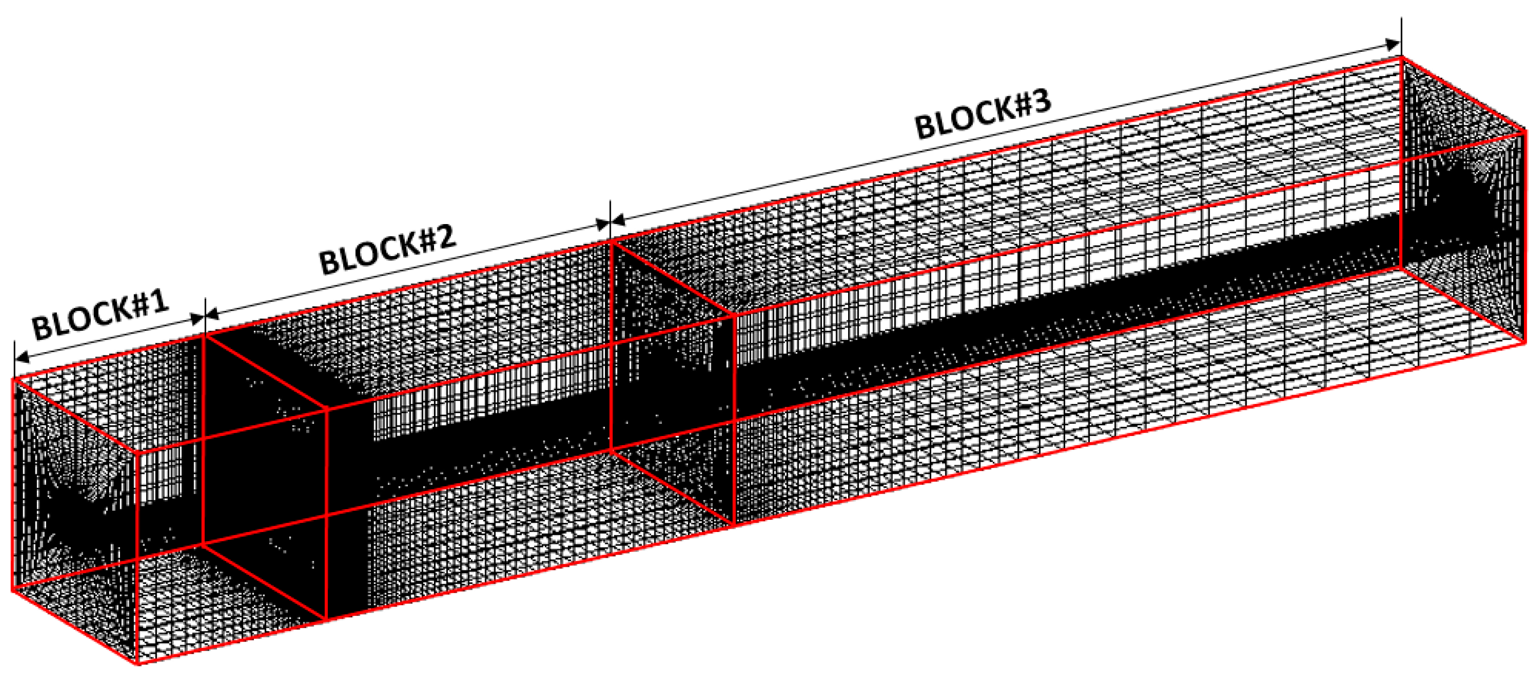
2.2. Numerical Method for Homogeneous Mixture Model

In the case of the homogeneous mixture model, since the volume fraction of the gas phase and the liquid phase are mixed, this makes the mach number 1.0 or higher even at low speed conditions due to different sound velocity conditions between the gas phase and the liquid phase. Numerical stiffness problems arise due to differences in sound velocity in each phase. This problem degrades convergence and causes a problem of diverging the solution, so an appropriate numerical analysis technique is required. In this study, the preconditioning technique was applied as shown in Equation (14). In Equation (14), the superscript ′ is a preconditioning parameter [2,4,5,17]. However, when the preconditioning method is applied, the accuracy of time is reduced. This change in time accuracy negatively affects the reliability of the analysis for unsteady-state flow. Therefore, the time accuracy was secured by applying the dual time stepping technique as shown in Equation (12). Applying this to Equation (1) is as follows [3,18]:
Γ e Q ^ t + Γ Q ^ τ + ( E ^ E ^ V ) ξ + ( F ^ F ^ V ) η + ( G ^ G ^ V ) ζ = S ^ .
Γe is a Jacobian matrix and Γ is a pre-conditioning matrix. The term t is physical time and τ is pseudo time. The Jacobian matrix and pre-conditioning matrix are given by:
Γ e = [ Y l ρ m p 0 0 0 Y l ρ m T ρ m + Y l ρ m Y v ρ m + Y l ρ m Y n g u ρ m p ρ m 0 0 u ρ m T u ρ m Y v u ρ m Y n g v ρ m p 0 ρ m 0 v ρ m T v ρ m Y v v ρ m Y n g w ρ m p 0 0 ρ m w ρ m T w ρ m Y v w ρ m Y n g h o ρ m p + ρ m h p 1 ρ m u ρ m v ρ m w h 0 ρ m T + h T h 0 ρ m Y v + ρ m h Y v h 0 ρ m Y n g + ρ m h Y n g Y v ρ m p 0 0 0 Y v ρ m T ρ m + Y v ρ m Y v Y v ρ m Y n g Y n g ρ m p 0 0 0 Y n g ρ m T Y g ρ m Y v ρ m + Y n g ρ m Y n g ]
Γ = [ Y l ρ m p 0 0 0 Y l ρ m T ρ m + Y l ρ m Y v ρ m + Y l ρ m Y n g u ρ m p ρ m 0 0 u ρ m T u ρ m Y v u ρ m Y n g v ρ m p 0 ρ m 0 v ρ m T v ρ m Y v v ρ m Y n g w ρ m p 0 0 ρ m w ρ m T w ρ m Y v w ρ m Y n g h o ρ m p + ρ m h p 1 ρ m u ρ m v ρ m w h 0 ρ m T + h T h 0 ρ m Y v + ρ m h Y v h 0 ρ m Y n g + ρ m h Y n g Y v ρ m p 0 0 0 Y v ρ m T ρ m + Y v ρ m Y v Y v ρ m Y n g Y n g ρ m p 0 0 0 Y n g ρ m T Y g ρ m Y v ρ m + Y n g ρ m Y n g ]
where
ρ m p = ρ m p + ( 1 c 2 1 c 2 ) ,
here c is the speed of sound in the mixture and c is the pseudo-speed of sound. The speed of sound is given by
c 2 = 1 ρ m p + 1 ρ m h p ρ m h T ρ m T .
The definition of the pseudo-sound speed is
( c ) 2 = min [ c 2 , max ( | U | 2 , β ) ] .
Here β is a parameter used as a performance benchmark of algorithm convergence to prevent the divergence of the calculation due to a too low convective propagation velocity. β = 1 is used in this study.
The constant CFL is used to restrict the time step for convergence. In the 3D multi-phase flow analysis based on the homogeneous mixture model, CFL was used as a reference to Ha [11], and 0.2 was used.

2.3. Turbulence Model

For the cavitation flow analysis, a filter-based k-ε model was used as the turbulence model. In the k-ε model, k represents the kinetic energy due to turbulence, and ε represents the dissipation rate due to turbulence.
ρ m d k d t = x j [ ( μ m + μ t σ k ) k x j ] + P k ρ m ε ,
ρ m d ε d t = x j [ ( μ m + μ t σ ε ) ε x j ] + c ε 1 P k ε k c ε 2 P k ε 2 k ,
where Pk is the production of turbulence defined as P k = τ i j ( u i / u j ) , and σk, σε, σε1, σε2, and cμ are the empirical constants. In this paper, the constants are used as σk = 1.0, σε = 1.3, σε1 = 1.44, σε2 = 1.92, and cμ = 0.09. This k-ε model is not suitable for an unsteady state due to excessive turbulent viscosity. To compensate for this, an improved turbulence model using a filtering method by Johansen was used. The grid size for filtering and the turbulent viscosity using it is expressed as follows [19]:
δ = ( Δ x Δ y Δ z ) ,
μ t = ρ m c μ M i n [ 1 , Δ · ε k 3 2 ] k 2 ε .

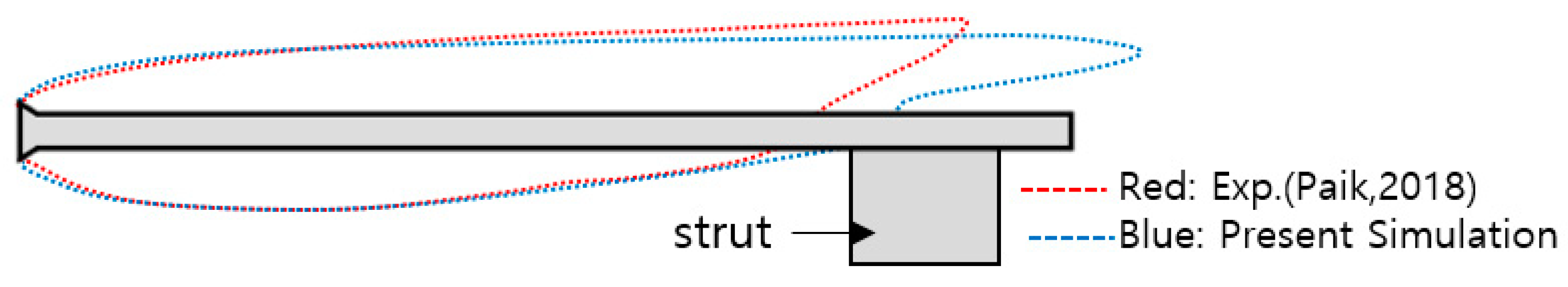
3. Ventilated Supercavitation Achievement

Cavitation is produced by a local pressure drop. When the speed of an object is high in the water, cavitation occurs to cover the body. The dimensionless number representing this physical phenomenon is the cavitation number. The cavitation number (σ) for the influent flow is as follows.
σ = P P V 1 2 ρ V 2 ,
where P is the pressure around the object or inflow, PV is the vapor pressure of water (fluid), ρ is the density of water (fluid), and V is the velocity in the direction of travel around the object or inflow. In general, the lower the cavitation number, the larger the size of the cavities. As V increases, σ decreases to achieve supercavitation. Achieving supercavitation by this method is called a natural supercavitation method.
Another way to reduce the cavitation number is to reduce the difference between inflow pressure and another. If gas is artificially injected, it can give a pressure change for cavitation production. The case of achieving supercavity by this method is called vetilated superacavitation, and the cavitation number can be defined as follows.
σ c = P P c 1 2 ρ V 2
where Pc is the pressure value in the cavitation formed by the artificially injected air, and when Pc, the pressure in the cavitation formed through the artificial injection, increases, ΔP decreases and, as a result, σc decreases. This enables supercavitation to be achieved even at low inflow velocity conditions. Normally, when the cavitation number is the same, the shape characteristic of the cavitation by natural cavitation and ventilated cavitation is known to be the same [5].
Therefore, in order to achieve supercavitation conditions by ventilation, gas injection is required. As the injection amount of gas increases, the ventilated cavitation number decreases and the cavitation shape fits the supercavition. At this time, the injection condition is related to the ventilated gas flux coefficient (Cq), and can be written as follows. In the case of the natural supercavitation, σ was reduced by increasing the thrust of the underwater vehicle.
C q = Q ˙ V d C 2 ,
where Q ˙ is the supply flow rate and dc is the cavitator diameter.
In this paper, we investigated the relationship between the ventilated cavitation resulting from the ventilated gas flux coefficient, the angle of attack of the cavitator and body velocity.

4. Numerical Results

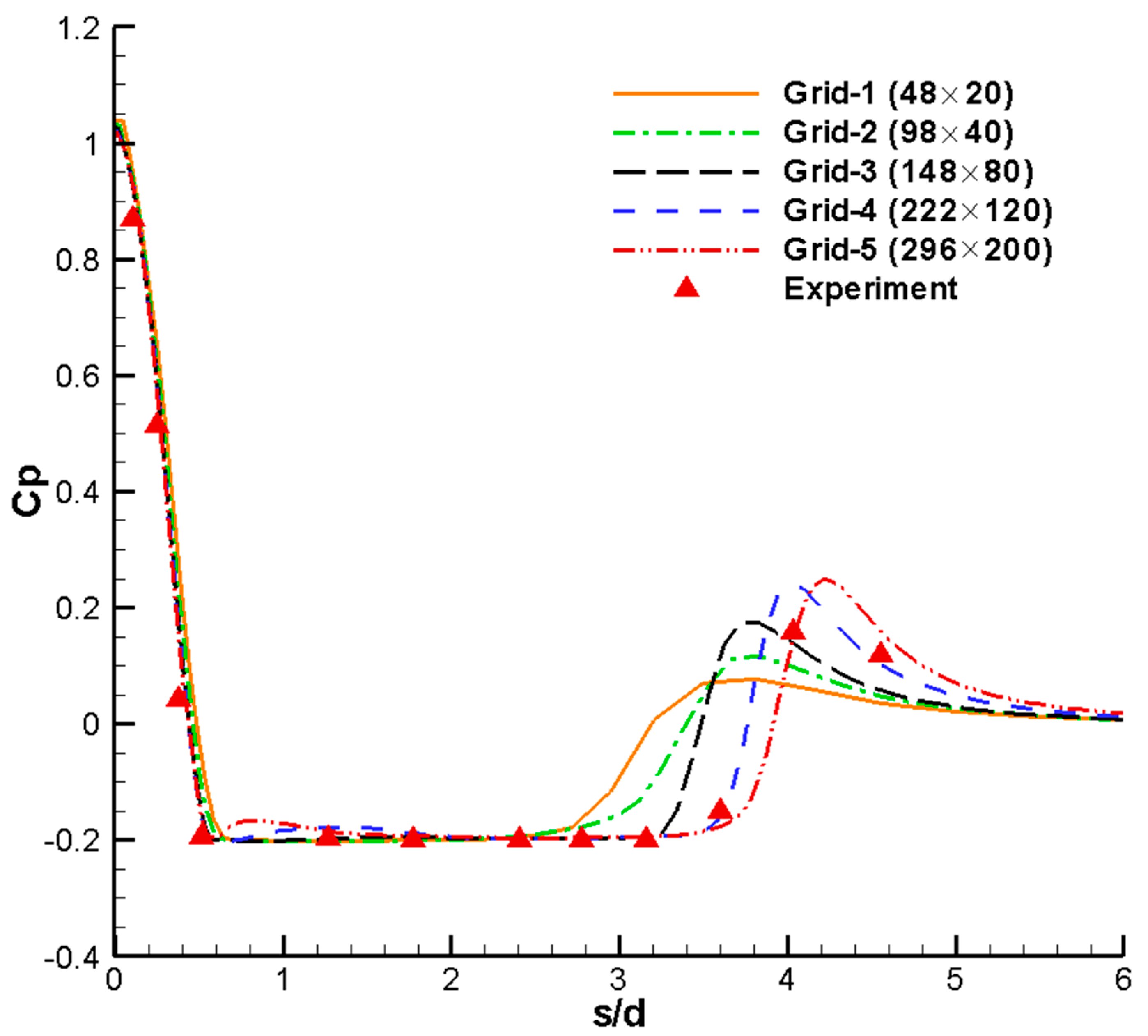
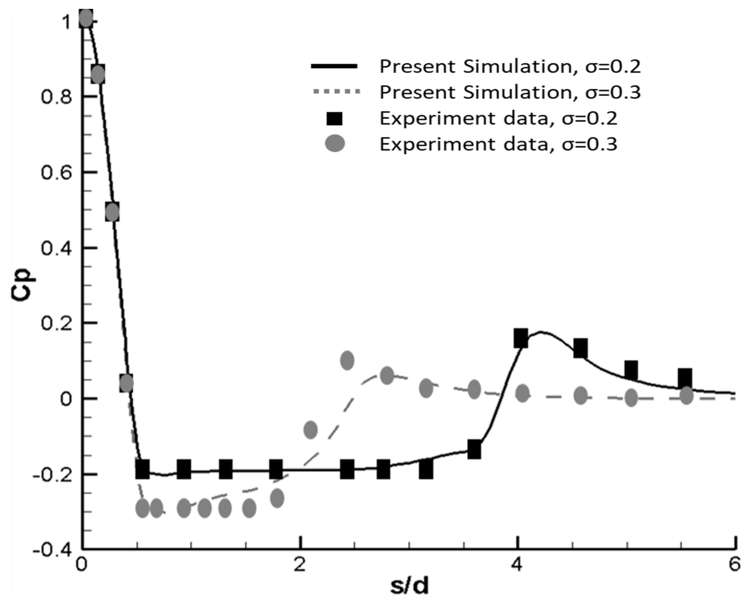
4.1. Natural Cavitation

Studies on natural cavitation have experimental data cited by many researchers [1], which have been verified in various ways [10,11]. In this paper, computational analysis of natural cavitation around a hemispherical head cylinder shape was performed using code developed in-house.
In this study, a grid sensitivity analysis was performed. It consists of a total of 5 steps of the grid and is as follows. Grid-1 (48 × 20 nodes), Grid-2 (98 × 40 nodes), Grid-3 (148 × 80 nodes), Grid-4 (222 × 120 nodes), and Grid-5 (296 × 200 nodes). Here, Grid-1 and Grid-2 are considered as the coarse grid, Grid-3 as the medium grid, and Grid-4 and Grid-5 as the fine grid. These grids use corresponding minimum grid sizes of 0.023, 0.009, 0.004, 0.0025 and 0.0015 in the normal direction near the wall. Figure 1 presents the time-averaged surface pressure coefficient distribution compared to that of the experiment. As can be seen from the results, grid resolution contributes to the prediction of cavitation dynamics. Current analysis results do not give good results on a coarse grid. The length of cavitation is predicted to be too short. The results of the medium grid show the quasi-stable state, and the results obtained with the fine grid show the unsteady behavior. As mentioned in Kinzel [20], improvements in the grid tend to improve cavitation dynamics and pressure solutions. In this paper, computational analysis was performed by applying a grid system that can define a fine grid based on the size near the wall.
Figure 2 compares the surface pressure coefficients at various cavitation numbers in experimental results [1] and analysis. The number s/d is dimensioned by the length and diameter of the hemispherical cylinder. The surface pressure coefficient (CP) is a dimensionless difference between the pressure on the surface and the ambient flow, and is generally multiplied by −1 to the result of Equation (18). When the cavitation number determined by Equation (16) is 0.2, CP cannot be lower than −0.2, and when the value is −0.2, it can be determined that a complete cavity is formed. When the number of cavities is 0.2 and 0.3, it is shown that the process of generating and developing cavities is in good agreement when comparing the experimental results with the analysis. There are some differences at the end of the cavitation because of the increased instability caused by the re-entrant jet occurring at the end of the cavitation. This is a physical phenomenon common to experiments and computational analysis. Figure 3 shows the results of the computational analysis of natural cavitation over time. Over time, the cavitation repeats the process of creation, destruction, and regeneration. The size of the cavitation shape is larger as the cavitation number is smaller. Also, since the natural cavitation is a phase change process caused by local pressure drop, it can be confirmed that the cavitation disappears as the pressure is restored. This is a very important physical phenomenon that is distinguished from ventilated cavitation through artificial injection.

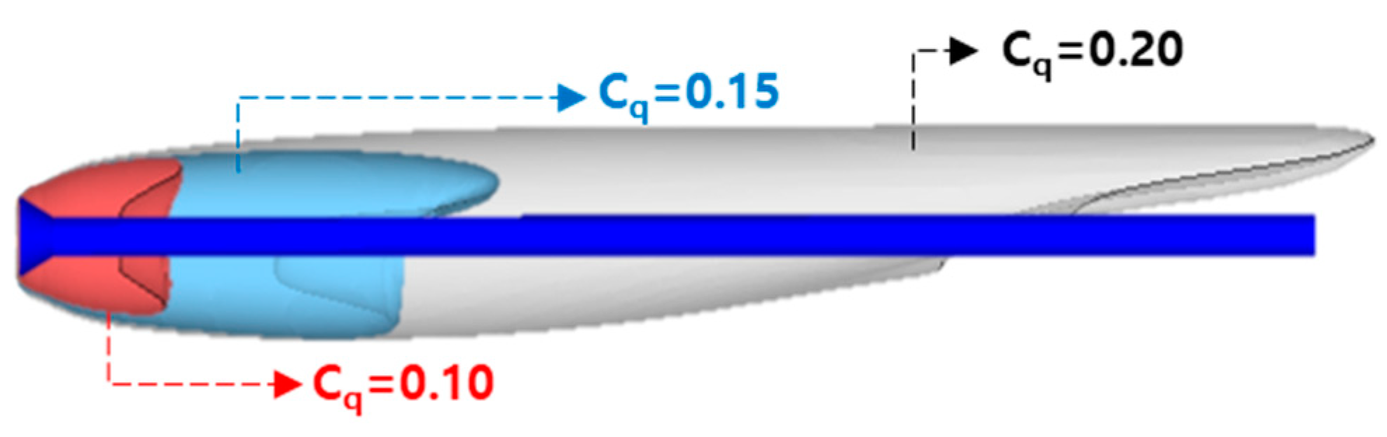
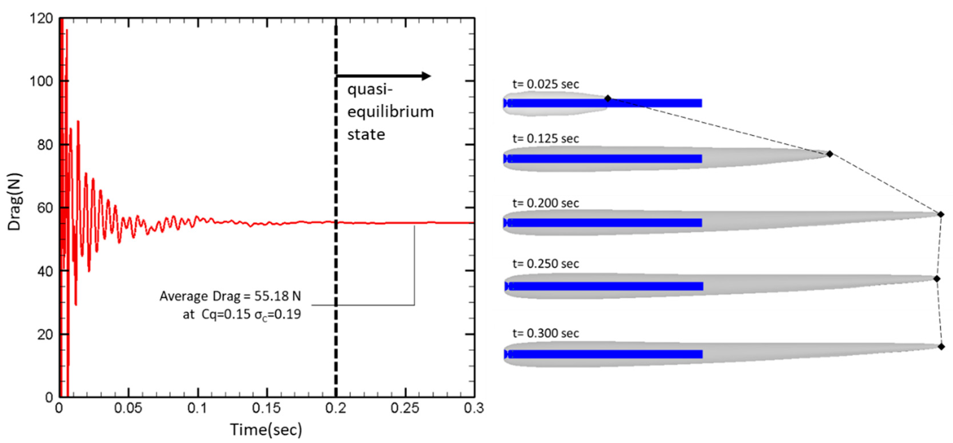
4.2. Ventilated Cavitation

For the supercavitation flow analysis, an alignment grid with three blocks is constructed. Figure 4 shows the entire grid system. The total number of cells is about 600,000. Many cells were placed around the cavitator and body to improve the stability and accuracy of the analysis. Figure 4 and Figure 5 show length information and boundary conditions for the entire grid. In the case of the front grid of the cavitator, if sufficient length is ensured, the flow can develop well and stably. However, in this study, only 10 times the diameter of the cavitator was secured because the size of the cavitation tunnel to be compared was modeled. The rear grid also considered the size of the cavitation tunnel. The value of D/dc = 9.49 was chosen to be identical to the environment in which the blockage effect affecting the cavitation size was verified. The boundary conditions include velocity inlet conditions and pressure outlet conditions. As an experiment for ventilated cavitation, conditions that do not generate natural cavitation are required. Therefore, in the experiment and analysis, the low speed (6 m/s) and total pressure (40 kPa) conditions are maintained. In the analysis, a ventilated area with the same area as the experiment was modeled. The four ventilated areas are evenly distributed along the body diameter. The ventilated area is the velocity inlet condition equal to the inflow condition. At this time, the ventilated velocity was determined by the ventilated gas flux coefficient.
Figure 6 shows the change of cavitation shape according to the change of Cq. In the experiment and analysis, the cavitation shape was confirmed after enough time had passed while Fn and Cq were kept constant. After enough time, the cavitation shape remains almost constant for a ventilated cavitation case [13]. Fn(= V / g d C ) is the flow field characteristic (gravity effect) according to the inflow velocity. The results of the computational analysis indicate that Fn is 10.8, which means low-speed conditions (V = 6 m/s). At this time, the shape characteristic of ventilated cavitation is asymmetric due to the buoyancy effect due to low Fn. When Fn is 10.8, it can be seen that the area of the cavitation covering the body increases as the ventilated gas flux coefficient increases, and the experimental and computational results are in good agreement. Figure 7 shows that when Fn is maintained and Cq is increased, the cavitation width and length become large. Since the increase in cavitation width is limited by the blockage effect, it can be confirmed that the length increase is relatively large. Figure 8 shows the result of comparing experiments and analysis for cavitation formation when Fn is 10.8 and Cq is 0.2. Experiment and analysis agree well except for the closing part of the cavity. This difference is the strut with and without. In the case of the experiment, there was a strut, but the analysis did not include the strut in the modeling. In the experiment, the strut inhibits the development of cavitation. In contrast, in analysis, there is no strut, so cavitation develops backward. This causes differences in the closing part of the cavitation.
In this study, computational analysis was performed not only of the cavity shape, but also of the drag force in the injection cavity. The following Figure 9 models for drag analysis. The shapes of the cavitator, body, and ventilated areas are modeled with reference to the shape of the test [13]. Figure 10 is the result of computational analysis of the drag coefficient value according to the change in the injection cavitation number. The drag coefficient is given by
C D = D r a g 1 2 ρ w a t e r V 2 A ,
where A is the area of the cavitator facing the flow. Drag is the sum of both form drag by pressure and skin friction due to viscosity.
It can be seen that the results of the cavitation tunnel test and computational analysis are in good agreement. As the injection amount increases, the cavitation number decreases and approaches the supercavitation. According to the cavitation shape change from the experimental and analysis results, it can be confirmed that the supercavitation occurs when the cavitation number is below 0.23. It can be confirmed by tests and computational analysis that the CD value is maintained at a certain level when it is supercavitation. In the case of the drag, there is no change after the supercavity is achieved, but the cavitation shape changes. In Figure 10, when the cavitation number is 0.19 and 0.21, the drag coefficient values are the same, but the cavitation length is different. In the case of the partial cavitation, instability by the re-entrant jet and the influence of the strut in Figure 8 exist, so the test and the analysis are not completely consistent. When the Cq is small and cavitation number high, the instability is expected to be greater. This difference can be seen in Figure 10 when the cavitation number is the largest. In order to minimize this instability in the computational analysis, the average value when the cavitation change reached the quasi-equilibrium state was employed. Figure 11 shows the results of computational analysis of the drag change and cavitation shape over time in a state where the cavitation number reaches 0.193. In the case of computational analysis, the flow field remains stationary until the analysis begins. At the same time as the analysis begins, the inflow is given a constant velocity value without acceleration. Therefore, the initial perturbation can be regarded as meaningless data that can occur numerically. To reduce uncertainty, the average value for data after 0.2 s was used as the result value for the condition. In the case of natural cavitation, the creation and destruction of cavitation are repeated, and the re-entrant jet occurs (see Figure 3). However, when the ventilated cavitation is continuously supplied with air, the cavitation shape is almost constant after the quasi-equilibrium state. In the cavitation shape analysis result on the right of Figure 11, the dotted line connects the cavitation end change over time. After 0.2 s, which is the quasi-equilibrium state, it can be confirmed that there was little change in the length of cavitation. These results indicate that in the case of ventilated cavitation when the gas is constantly supplied, the cavitation shape is independent of the time variable. In this case, the CPU time is approximately 44 h from the start of analysis to the semi-equilibrium state (0.2 s). The total CPU time up to 0.3 s is about 65 h (Xeon E5-2640, 2.40 GHz).

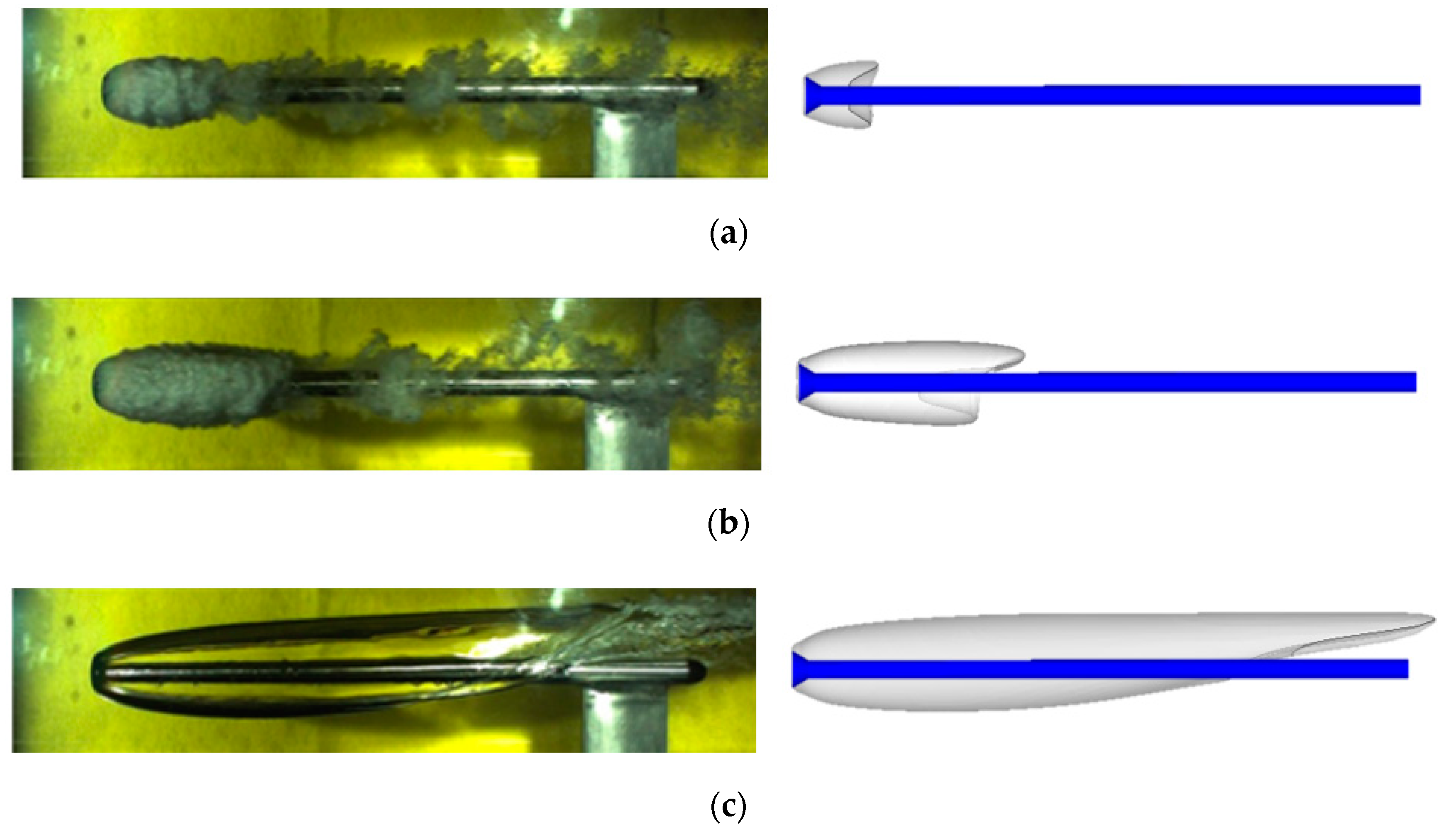
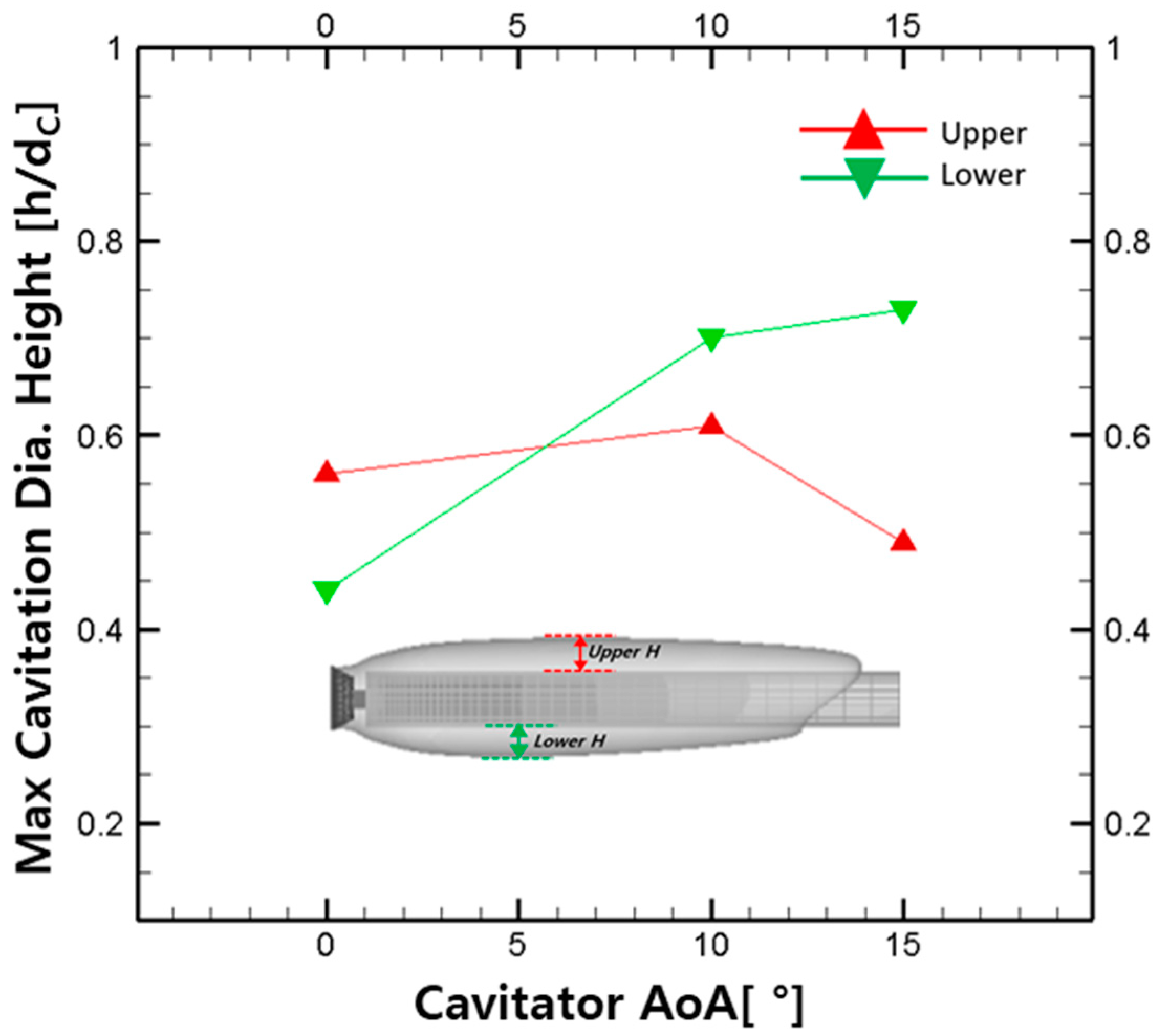
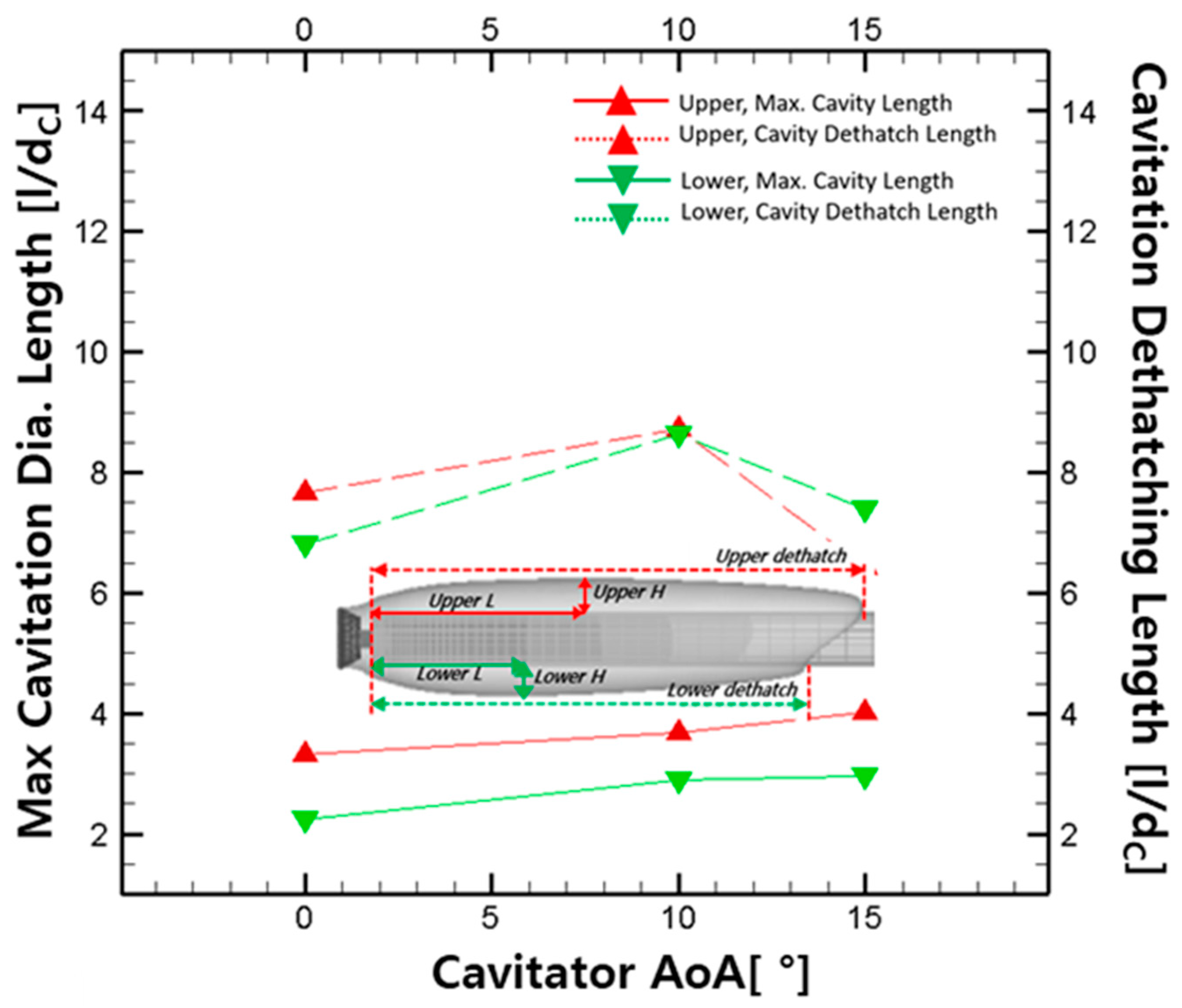
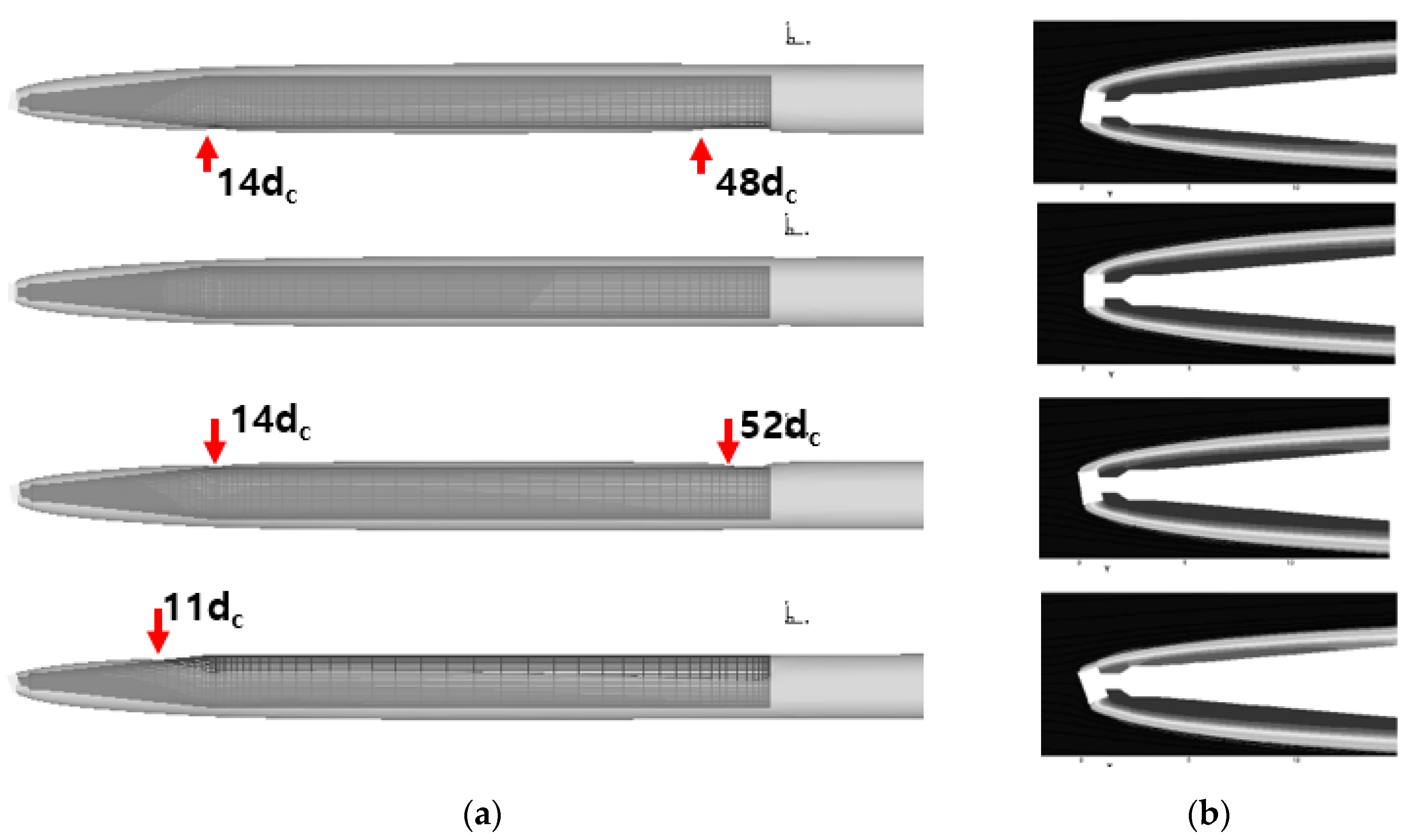
4.3. Cavitation Shape with Cavitator Angle of Attack

Factors that determine the maximum diameter and length of the cavitation are Fn at ambient speed and Cq and σC at the injection rate. In addition, there are angles of attack of the cavitator that can have a very large impact in real environments. In this study, we studied how the shape of cavitation changes when the cavitator has an angle of attack. Figure 12 shows the cavitation shape change according to the angle of attack of the cavitator in the injection cavitation computational analysis with the injection characteristic of Cq = 0.15.
When the angle of attack (AoA) is 0°, the cavitation asymmetry due to the rise of the cavitation tail due to the gravity and buoyancy effect occurs as shown in Figure 6. If the angle of attack is 10 degrees, the cavitation generated from the cavitator is generated below the body, thereby canceling the asymmetry of the cavitation trailing edge caused by buoyancy. When the angle of attack is 15°, the cavitation shape becomes more prominent, and it can be seen that the cavitation covers more area under the body. Figure 13 shows the height (h) from the body surface to the maximum cavitation diameter with the cavitator angle. The maximum cavitation diameter means the largest point formed on the upper and lower, respectively. As the cavitator angle increases, the asymmetry of the cavity is formed with a larger distance from the lower surface to the cavitation maximum diameter. In the case of the upper surface, when the angle is 15 degrees, the distance to the maximum diameter of the cavitation is greatly reduced. Figure 14 shows the length of the shape of the cavity according to the angle of attack. The solid line indicates the distance to the point where the maximum cavitation occurs. As the cavitator angle increases, it can be seen that it increases slightly without significant difference. The dotted line represents the cavitation dethatching length. When there was no angle of attack, the upper length was longer. However, as the angle of attack increased, the upper length and lower length became the same and eventually reversed. Being able to predict the length of the cavitation according to the angle of attack is important information in maintaining the super cavitation. Asymmetric formation of cavitation with changes in cavitator angle is related to body shape characteristics. In the case of the analyses of Figure 12, Figure 13 and Figure 14, the diameter of the cavitator is similar to that of the body, so the cavitation generated from the cavitator propagates well backward. As shown in Figure 15, in real scale the diameter of the body is larger than the diameter of the cavitator. In this geometry, the change in cavitation size caused by the angle of attack of the cavitator can have a significant effect on the body’s motility. Figure 15 shows the result of changing the angle of attack to −10°, +10°, and +20° for the case of the super cavitation formed around the high-speed underwater vehicle. At 0°, there is no wetted surface where water and body come in contact with anything other than the front of the cavitator. In addition, it can be confirmed that the cavitation asymmetry does not occur due to the buoyancy effect as shown in Figure 12 even though the angle of cavitation is 0° due to the high-speed condition. In this case, when the angle of attack has a value of 10° in the upward direction, the generation of the cavitation to the lower surface is limited. Therefore, the receiving surface, where the cavitation is destroyed and the water and the body come into contact, occurs at 14dc from the front. The destroyed cavitation will recover and cover the body again, but one can see that the receiving surface occurs once again at 48 dc. This phenomenon is similar to the above result when the angle of attack has a value of 10° in the downward direction, because the buoyant effect is insufficient at high-speed conditions and the cavities and the body are symmetrical in shape. If the angle of attack increased further to 20°, the fractured cavitation in the upper surface exited the body without recovering again, resulting in a large wetted surface. This increase in wetted surface means that the body suddenly receives resistance due to the very large density difference between liquid and vapor. This is a very serious problem in terms of coordination of the body’s motion, so it is important to maintain the cavitation well. Therefore, the cavitation shape prediction according to the angle of attack becomes an important factor in the reorientation of the supercavitation moving body.

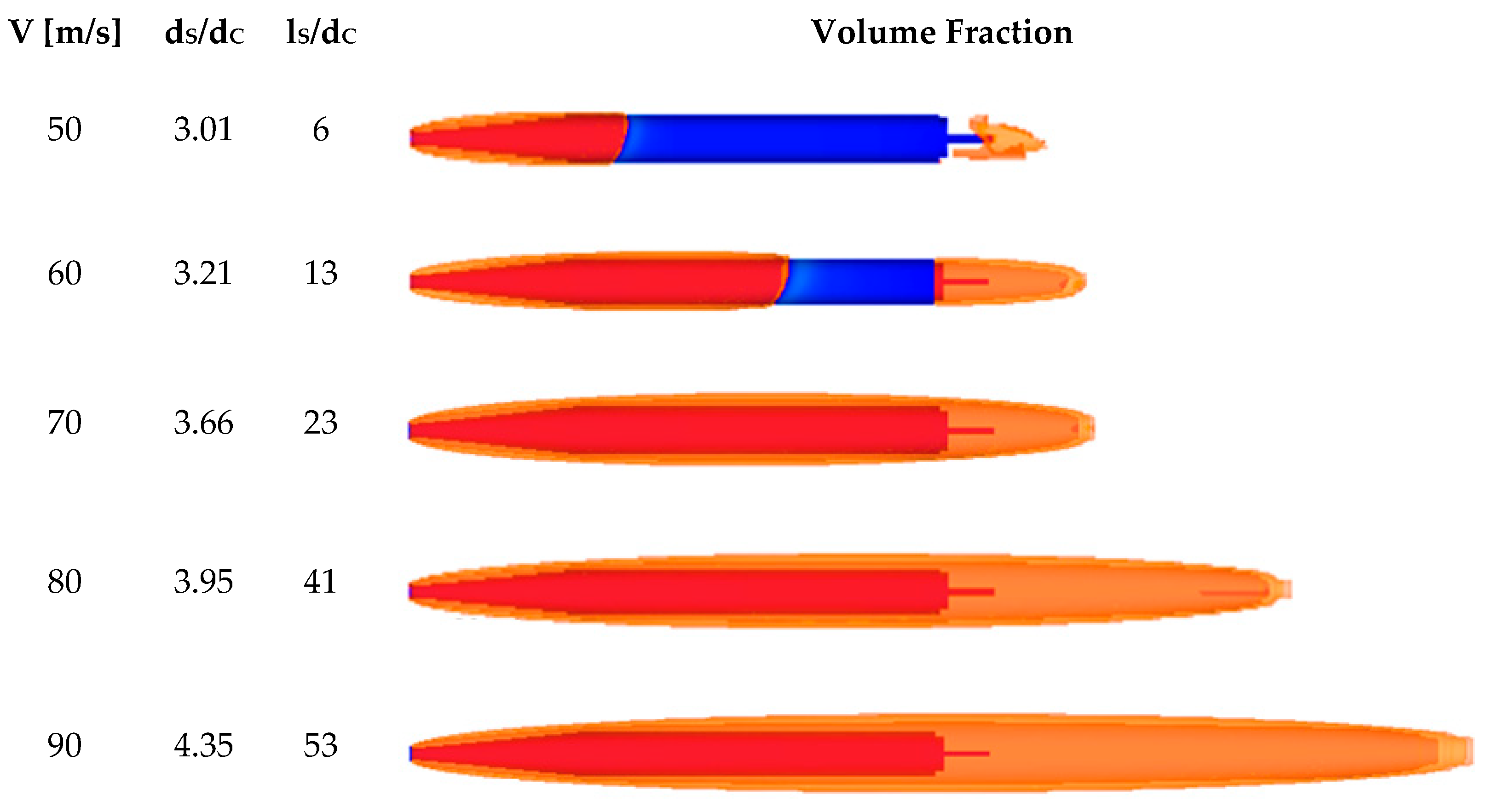
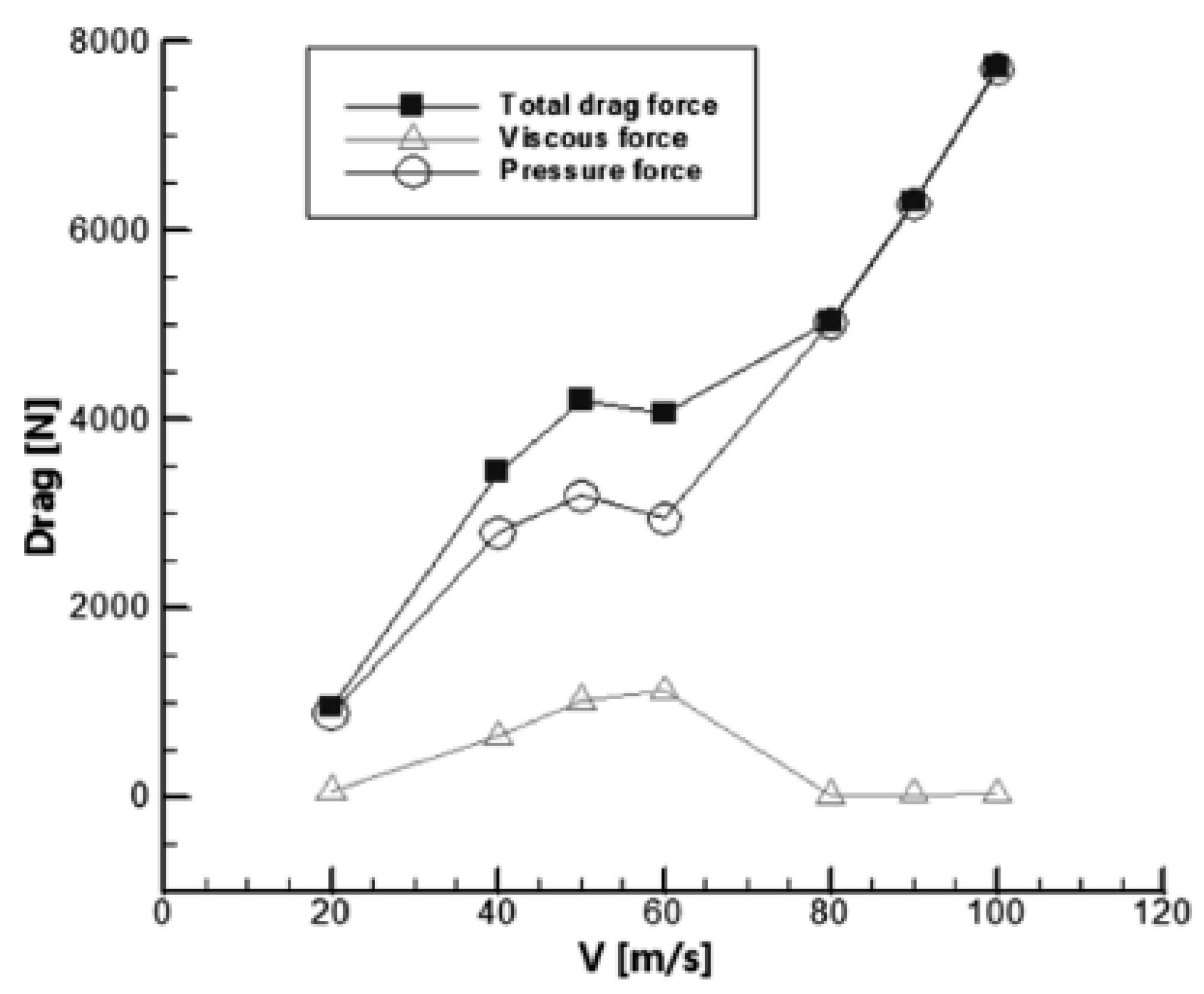
4.4. Cavitation and Drag Change According to Speed Variation

In this section, the computational analysis of the change of the cavitation shape according to the speed change was studied. For the underwater body to achieve a super cavitation only with a natural cavitation without the injection cavitation, it needs a speed higher than a certain speed. When supercavitation is achieved by these high speed conditions, the object can receive a large drag reduction effect.
Figure 16 shows the natural cavitation shape as the velocity increases. V is the velocity of inflow, dS is the maximum diameter of the cavitation, dC is the diameter of the cavitator, and lS is the maximum length of the caviation. In the case of a natural cavitation, it can be confirmed that the body speed is completely covered by the cavitation between 70 and 80 m/s. As the speed increased, the maximum diameter of the cavitation increased, and after 70 m/s, the cavitation generated from the front met the cavitation created in the tail, and the maximum length of the cavitation increased significantly. Figure 17 shows the total force of drag divided by the forces for pressure and viscous. The total drag is given by,
D r a g = p cos θ d A + τ sin θ d A ,
where θ is the angle to the flow direction and A is the microsurface area.
Figure 18, Figure 19 and Figure 20 show the results of time analysis of pressure and viscosity forces when the speed conditions are 50, 70, and 90 m/s, respectively. It can be assumed to be in a semi-equilibrium state from 0.05 s onward, starting from a stationary state, and then the average value is applied to Figure 16. The pressure force is a function of the magnitude of the pressure and the direction the surface acts on. In this case, since the cavitator is perpendicular to the flow, most of the pressure force occurs at the cavitator and the slope. The pressure force decreases in spite of increasing speed in the range of 40 to 60 m/s. The reason is that the cavitation develops completely covering the slope after the cavitator.
Figure 18 shows the results of the partial cavitation computational analysis with a speed of 50 m/s. The reason for the oscillation of the graph results is that the wetted surface continuously changes due to the partial cavitation, which is the result of the unsteady state analysis. The oscillation is more severe due to the cavitation shape falling off of the tail. Figure 19 is the result of the computational analysis of 70 m/s. This is the result of the computational analysis of the transition point from the partial cavitation to the supercavitation. Although not yet complete supercavitation, it can be seen that the viscous force is reduced compared to Figure 18 because it is close to the supercavitation state. Figure 20 shows the force in a complete super cavitation as a result of the computational analysis of 90 m/s. As the speed increases, the pressure force is increased by the exposed head, but it can be seen that the viscous force is completely removed due to the complete supercavitation. By the relationship between the supercavitation and the viscous force, the supercavitation contributes to lowering the level of the total force.

4.5. Ventilated Cavitation with High Speed Underwater Vehicle

In the case of a natural cavitation, a velocity condition higher than a certain value is required to achieve a super cavitation. However, if the injection cavitation is used as in Section 4.2, a super cavitation can be achieved even at low-speed conditions. The velocity condition in Figure 21 is 30 m/s. It can be seen from the results of Figure 16 that the supercavitation cannot be reached when the velocity condition is 30 m/s. However, the artificially injected cavitation in front of the body makes this possible. It can be seen that the gas injected from the front of the body forms a cavitation and covers the entire body in a very short time. The injected gas is a non-condensing gas, which is transmitted to the rear, and it can be seen that the rear end cavitation rises upward due to the buoyancy effect in the low-speed condition. This is a physically valid result even when compared with the results in Figure 5, Figure 6 and Figure 7. However, because the body itself is low in speed, even if the super cavitation is achieved, the problem is that the maximum diameter of the cavitation is small and the tail cavitation is short compared to the super cavitation shape of 80 m/s or more in Figure 16. However, since the injection cavitation can achieve super cavitation even at low-speed conditions, it is expected that it can be used to assist and maintain the formation of the initial super cavitation in the design of the super-high-speed underwater vehicle.

5. Conclusions

This study is the result of the multi-phase flow field analysis including supercavitation phenomena, using a 3D Navier-Stokes equation based homogeneous mixture model. For the verification of the analysis program, natural and ventilation cavities were tested respectively. In the case of the natural cavitation, the results of previous researchers’ results were compared with the results of computational analysis, and it was confirmed that the cavitation shape was in good agreement. The ventilation cavitation was compared with the experimental results. It was confirmed that the experimental and analysis results, according to the change of the ventilation coefficient, were in good agreement. As a result, it was confirmed that the analysis program had sufficient suitability to analyze both natural and ventilation cavitations. In addition, a computational analysis of the drag force in the quasi-equilibrium state was performed and compared with the experiment. The results show good agreement.
Using the verified code, the shape of the cavitation according to the angle of attack was studied for the experimental scale and the actual scale, respectively. In the experimental scale, there was a limitation of the speed condition, so it was possible to confirm the cavitation asymmetry phenomenon caused by the buoyancy effect. The paper also analyzed how these cavitation asymmetries change with the angle of attack. It was confirmed that the asymmetric phenomenon caused by buoyancy did not occur in the high-speed condition of the actual scale shape.
Computational analysis was performed to increase the speed on an actual scale. As the velocity increased, the width and length of the cavity were expressed as a dimensionless number by the cavitator diameter. At this time, the total resistance was expressed by dividing it into pressure resistance and viscous resistance. This shows why the drag reduction effect caused by supercavitation occurs. Finally, it was confirmed that supercavitation was achieved by performing computational analysis of ventilated cavitation on the actual shape.
It is thought that these research results and verified programs could contribute to engineering in the case of using super-cavitation phenomena such as super-high-speed water bodies in the future.

Author Contributions

Conceptualization, W.-G.P.; formal analysis, D.-H.K.; funding acquisition, W.-G.P.; investigation, D.-H.K.; methodology, D.-H.K. and W.-G.P.; project administration, D.-H.K. and W.-G.P.; software, D.-H.K. and S.S.P.; supervision, W.-G.P.; validation, D.-H.K.; writing—original draft preparation, D.-H.K. and S.S.P.; writing—review and editing, D.-H.K. and W.-G.P. All authors have read and agreed to the published version of the manuscript.

Funding

This work was supported by National Research Foundation of Korea (NRF) grant funder by the Korea government (MIST) (NRF-2018R1A2B6008864) and the Human Resources Development program (No. 20184030202060) of the Korea Institute of Energy Technology Evaluation and Planning (KETEP) grant funded by the Korea government Ministry of Trade, Industry and Energy.

Conflicts of Interest

The authors declare no conflict of interest.

References

  1. Rouse, H.; McNown, J.S. Cavitation and Pressure Distribution: Head Forms at Zero Angle of Yaw; State University of Iowa: Iowa City, IA, USA, 1948. [Google Scholar]
  2. Kunz, R.F.; Lindau, J.W.; Billet, M.L.; Stinebring, D.R. Multiphase CFD Modeling of Developed and Supercavitaing Flows. In Proceedings of the Von Karman Institute, Special Course on Supercavitating Flows, Rhode-Saint-Genese, Belgium, 12–16 February 2001; RTO EN-013. pp. 12–16. [Google Scholar]
  3. Ahuja, V.; Hosangadi, A.; Arunajatesan, S. Simulation of cavitating flow using hybrid unstructured meshes. J. Fluids Eng. 2001, 123, 331–340. [Google Scholar] [CrossRef]
  4. Kunz, R.F.; Boger, D.A.; Stinebring, D.R.; Chyczewski, T.S.; Lindau, J.W.; Gibeling, H.J.; Venkateswaran, S.; Govindan, T.R. A preconditioned Navier-Stokes method for two-phase flows with application to cavitation prediction. Comput. Fluids 2000, 29, 849–875. [Google Scholar] [CrossRef]
  5. Kunz, R.F.; Boger, D.A.; Chyczewski, T.S.; Stinebring, D.R.; Gibeling, H.J.; Govindan, T.R. Multi-phase CFD analysis of natural and ventilated cavitation about submerged bodies. ASME Pap. FEDSM 1999, 99, 7364. [Google Scholar]
  6. Lindau, J.W.; Venkateswaran, S.; Kunz, R.F.; Merkle, C.L. Computation of compressible multiphase flows. In Proceedings of the 41st Aerospace Sciences Meeting and Exhibit, Reno, NV, USA, 6–9 January 2003; p. 1285. [Google Scholar]
  7. Lindau, J.W.; Kunz, L.F.; Venkateswaran, S.; Stinebring, D.R. Homogeneous multiphase CFD modeling of large scale cavities. In Proceedings of the ECCOMAS 2004, Jyväskylä, Finland, 24–28 July 2004. [Google Scholar]
  8. Merkle, C.L.; Feng, J.Z.; Buelow, P.E.O. Computational modeling of the dynamics of sheet cavitation. In Proceedings of the 3rd International Symposium on Cavitation, Grenoble, France, 7–10 April 1998; pp. 307–311. [Google Scholar]
  9. Owis, F.M.; Nayfeh, A.H. Computations of the compressible multiphase flow over the cavitating high-speed torpedo. J. Fluids Eng. 2003, 125, 459–468. [Google Scholar] [CrossRef]
  10. Kim, D.H.; Park, W.G.; Jung, C.M. Numerical simulation of cavitating flow past axisymmetric body. Int. J. Naval Archit. Ocean Eng. 2013, 4, 256–266. [Google Scholar] [CrossRef]
  11. Ha, C.T.; Park, W.G. Evaluation of a New Scaling Term in Preconditioning Schemes for Computations of Compressible Cavitating and Ventilated Flows. Ocean Eng. 2016, 126, 432–466. [Google Scholar] [CrossRef]
  12. Ahn, B.K.; Jeing, S.W.; Kim, J.H.; Shao, S.; Hong, J.; Arndt, R.E.A. An Experimental Investigation of Artificial Supercavitation Generated by Air Injection Behind Disk-shaped Cavitator. Int. J. Naval Archit. Ocean Eng. 2016, 9, 227–237. [Google Scholar] [CrossRef] [Green Version]
  13. Paik, B.G.; Lee, S.J.; Ahn, J.W.; Kim, K.S.; Baek, B.K.; Jeong, Y.R.; Kim, K.Y.; Ahn, J.W.; Seol, H.S.; Ki, S.K. Fundamental Studies for Ventilated Supercavitation Experiments in New High-speed Cavitation Tunnel. J. Soc. Naval Archit. Korea 2018, 55, 330–340. [Google Scholar] [CrossRef]
  14. Ha, C.T.; Park, W.G. Application of preconditioning to compressible multi-phase mixture flow computation. In Proceedings of the 5th International Symposium on Fluids Machinery and Fluids Engineering, Jeju, Korea, 24–27 October 2012; pp. 24–27. [Google Scholar]
  15. Ha, C.T.; Kim, D.H.; Park, W.G. A compressive interface-capturing scheme for computation of compressible multi-fluid flows. Comput. Fluids 2017, 152, 164–181. [Google Scholar]
  16. Ha, C.T.; Park, W.G.; Merkle, C.K. Multiphase flow analysis of cylinder using a new cavitation model. In Proceedings of the 7th International Symposium on Cavitation, CAV2009, Ann Arbor, MI, USA, 16–18 August 2006; p. 99. [Google Scholar]
  17. Owis, F.; Nayfeh, A. Numerical simulation of super-and partially-cavitating flows over an axisymmetric projectile. In Proceedings of the 39th Aerospace Science Metting and Exhibit, Reno, NV, USA, 8–11 January 2001; p. 1042. [Google Scholar]
  18. Lindau, J.W.; Kunz, R.F.; Venkateswaran, S.; Merkle, C.L. Development of a fully—Compressible multiphase Reynolds Navier–Stokes model. In Proceedings of the 15th AIAA Computational Fluid Dynamics Conference, Anaheim, CA, USA, 11–14 June 2001; pp. 11–14. [Google Scholar]
  19. Johansen, S.T.; Wu, J.; Shyy, W. Filter-based unsteady RANS computations. Int. J. Heat Fluid Flow 2004, 25, 10–21. [Google Scholar] [CrossRef]
  20. Kinzel, M.P. Computational Techniques and Analysis of Cavitating-Fluidflows; The Pennsylvania State University: State College, PA, USA, 2008. [Google Scholar]
Figure 1. Sensitivity of grid resolution to surface pressure prediction.
Applsci 10 04228 g001
Figure 2. Surface pressure coefficient on the hemispherical head cylinder at various cavitation numbers.
Applsci 10 04228 g002
Figure 3. Analysis of changes in natural cavitation shape over time in two cavitation numbers.
Applsci 10 04228 g003
Figure 4. Computational grid for underwater vehicle.
Applsci 10 04228 g004
Figure 5. Schematric view of the computational model and boundary conditions.
Applsci 10 04228 g005
Figure 6. Cavitation formation at various ventilated rate coefficients: (a) Fn = 10.8, Cq = 0.10, (b) Fn = 10.8, Cq = 0.15, and (c) Fn = 10.8, Cq = 0.20. (Abbreviations: gas flux coefficient (Cq), flow field characteristic (Fn))
Applsci 10 04228 g006
Figure 7. Cavitation formation at various ventilated rate coefficients.
Applsci 10 04228 g007
Figure 8. Cavitation formation at various ventilated rate coefficients (Fn = 10.8, Cq = 0.20).
Applsci 10 04228 g008
Figure 9. Schematric view of the computational model and cavitation shape for σc = 0.19.
Applsci 10 04228 g009
Figure 10. Comparison of drag coefficient according to the various ventilated supercavitations.
Applsci 10 04228 g010
Figure 11. Result of computational analysis of drag change and cavitation shape over time (Cq = 0.152).
Applsci 10 04228 g011
Figure 12. Cavitation formation at various cavitator angles of attack (Cq = 0.15, angle of attack = 0, 10, 15°).
Applsci 10 04228 g012
Figure 13. Comparison of maximum cavitation diameter for various cavitator angles of attack.
Applsci 10 04228 g013
Figure 14. Comparison of length for maximum cavitation diameter and dethatch for various cavitator angles of attack.
Applsci 10 04228 g014
Figure 15. Real scale underwater body cavitation formation at various cavitator angles of attack (angle of attack = −10°, 0°, 10°, 20°): (a) cavity shape and point of collapse (−10°, 0°, 10°, 20°), and (b) cavitator angle of attack (−10°, 0°, 10°, 20°).
Applsci 10 04228 g015
Figure 16. Prediction of supercavitation shape according to velocity change.
Applsci 10 04228 g016
Figure 17. Prediction of drag change according to velocity change.
Applsci 10 04228 g017
Figure 18. Analysis of drag unsteady state pressure force and viscous force at 50 m/s.
Applsci 10 04228 g018
Figure 19. Analysis of drag unsteady state pressure force and viscous force at 70 m/s.
Applsci 10 04228 g019
Figure 20. Analysis of drag unsteady state pressure force and viscous force at 90 m/s.
Applsci 10 04228 g020
Figure 21. Prediction of ventilated super cavitation shape change over time.
Applsci 10 04228 g021

