Abstract
A separated foundation model was proposed in order to reduce the calculation scale of the numerical model for analyzing soil-bridge structure dynamics. The essence of the wave input analysis model considering soil-structure interaction was analyzed. Based on the large mass method, a one-dimensional time-domain algorithm of the free field was derived. This algorithm could simulate the specified ground motion input well. The displacement expansion solution of the free wave field was solved based on the propagation law of waves in a medium. By separating the soil foundations around the pile foundations of the bridge, the ground motion was transformed into an equivalent load applied on an artificial boundary. The separated foundation model could consider the incoherence effect and soil-structure interaction simultaneously; the number of model elements were reduced, and the computational efficiency was improved. In order to investigate the seismic response of a curved bridge considering soil-structure interaction under spatially varied earthquakes, a curved bridge with small radius was adopted in practical engineering. Spatially correlated multi-point ground motion time histories were generated, and the nonuniform ground motion field was simulated based on the wave input method on an artificial viscoelastic boundary. The effects of different apparent wave velocities, coherence values, and site conditions on the seismic response of the bridge were analyzed. The results showed that the spatial variation of seismic ground motion had a considerable effect on the bending moment and the torsion of the girder. The site effect had great influence on the bending moment of the pier bottom. When considering soil-structure interaction, the spatial variation of ground motion should be fully considered to avoid underestimating the structural response.
1. Introduction
Curved bridges are common in many cities and mountainous areas because of their good landscape and environmental adaptability, especially at graded intersections and space-limited overpass bridges. However, such bridges are more susceptible to earthquake-induced damage than conventional bridges, mainly because of their irregular geometry and uneven mass distribution. Studies have shown that the spatial variability of ground motions will have adverse effects on curved bridges [1]. Although during many earthquakes, curved bridges have incurred severe damage, most of the current seismic specifications, including the American AASHTO Seismic Design Guide (AASHTO 2011) and Caltrans Seismic Design Standard (Caltrans 2010) and the Highway Bridge Seismic Design Specifications 2008, did not make recommendations or take measures to avoid these problems. This is because of the lack of complete understanding of the dynamic performance of curved bridges during earthquakes. During the Wenchuan earthquake in China, many ramp bridges with small radii collapsed, but the main bridge remained almost intact [2]. In view of the novel geometrical characteristics of small-radius curved bridges and the lack of relevant regulations, it is particularly important to carry out a comprehensive and systematic analysis of the behavior of such bridges under ground motion with spatial variation.
Few researchers have reported about the seismic response of curved bridges under ground motion with spatial variation. Desroches [3] pointed out the importance of considering multi-support input with the actual curved bridge collapse. Chen Yanjiang and Wang Jinjie [4] studied the response of curved girder bridges under ground motion with spatial variation from the perspective of random vibration angles. Sextos and Kappos [5] analyzed the seismic response of curved bridges under multi-support excitation by synthesizing multi-support ground motion. Burdette and Elnashai [6] compared the influence of the traveling wave and incoherence on the seismic response of curved bridges and regular bridges. Through shaking table tests, Li Xi and Jia Hongyu [7] found that the traveling wave effect affects curved bridges more adversely than straight bridges. Cheng Maili and Li Qingning [8] pointed out through the shaking table test that the influence of multi-support excitation effect should be considered in the seismic analysis of irregular high-rise curved beam bridges. However, most of the current studies have not considered the soil-structure dynamic interaction, and the seismic real response of the structure is quite different from that of the base fixed model [9].
With regard to models considering soil-structure interaction. There are still many problems unsolved, and many researchers are still actively exploring this field [10,11,12,13]. Dai Gonglian and Liu Wenshuo [14] used the m method to establish a curved beam bridge finite element model. However, it is cumbersome to define a large number of simulated soil-structure interaction units and pre-calculate the ground motion time history of the horizontal position of different units. Sextos and Taskari [15] studied the effects of multi-angle input on the seismic responses of curved beam bridges based on the refined finite element model. Ye Aijun and He Jian [16] proposed a seismic response analysis method for the site-structure integral model for bridges with pile foundations. However, in references [17,18], a consistent acceleration or displacement time history at the bottom of the model was employed and artificial boundaries were laterally introduced, without considering the non-uniform input of ground motion. The fundamental features of the seismic soil-structure interaction on the response of pile-supported structures are investigated [17]. Papadopoulos [18] transformed ground motion into an equivalent load acting on the bottom and side boundaries of the overall model to simulate the ground motion input field; however, the input equivalent load satisfies the displacement boundary conditions only but not the force boundary conditions, resulting in some errors in the result. Liu Jingbo and Tan Hui [19] obtained the artificial boundary equivalent load by adopting the substructure dynamic analysis method, which has the same precision as the wave input method. It is necessary to pre-establish the substructure model to calculate the equivalent load on an artificial boundary.
There are significant differences in ground motion, such as differences in amplitude, spectral composition, and arrival time of ground motion, at different points on the ground. However, studies have shown that the results obtained from the seismic response analysis are conservative if the effects of ground motion spatial variations are not considered [20,21]. Because of the obvious spatial characteristics of the seismic responses of curved beam bridges, the numerical model of the dynamic interaction of the whole soil-bridge structure considering the foundation and soil has a large scale. In fact, all the information obtained in a bridge engineering survey forms the site data near the pile foundation. Therefore, it is necessary to simplify the numerical model of the overall soil-bridge structure in order to reduce the size and calculation.
At present, the soil and pile combined with the bridge structure have not been considered in one numerical model, and the seismic research of the curved beam bridge has not been carried out. For curved bridges, multiple points inputs and pile-soil interactions will have a greater impact on the structure. The method proposed in this paper presents a feasible method for curved beam bridges considering multi-point seismic effects, multi-directional seismic input and pile-soil interaction.
A separated foundation-bridge system model is proposed. In addition to the ground motion correlation at each point, the model can also consider the pile-soil interaction, thereby considerably reducing computational space and calculation time. The wave input model was analyzed. Based on the mass method, the one-dimensional time domain algorithm of free field was derived. The displacement expansion solution of the free field was solved based on the wave propagation law in the medium and Snell’s law. Thereafter, the ground motion was transformed into an equivalent load on the artificial boundary, and the equivalent load was calculated by the compiled auxiliary calculation program. The spatial correlation multi-support ground motion time history was synthesized. The seismic performance of the curved beam bridge under the action of spatially varying earthquakes was systematically studied using the proposed model. The effects of different apparent wave velocities, degrees of coherence, and site conditions on the seismic performance of the structures were considered.
2. Wave Input Calculation Model
Pile-soil dynamic interaction is a classic problem. Research has been carried out for many years. There are mainly two directions of research in this area. One is to combine the Fourier transform in the frequency domain for research. The other is to consider the whole of soil and structure and conduct research in the time domain. There are many studies on the former. In terms of vibration, research and testing in the frequency domain can be achieved. However, because it is difficult to consider nonlinear problems happened in soil, research based on the frequency domain under earthquake action has obvious limitations. The real soil should be simulated into the numerical model. Because of the seismic wave input and calculation amount of the overall model, it is difficult to consider the overall model of soil and structure in the time domain. A soil-structure dynamic interaction system is shown in Figure 1. Generally, when solving such problems, a certain range of soils on the structural foundation is cut out, and then, the artificial boundary elements are introduced into the finite element model to absorb the outer wave [22]. Simultaneously, a force boundary condition (Figure 2) is applied to the node. Therefore, the motion equation of the finite element model of the soil-structure dynamic interaction can be presented as shown in Equation (1).

Figure 1.
Schematic diagram of the soil-structure dynamic interaction system.
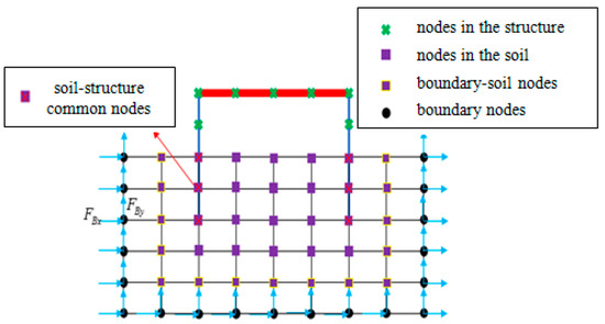
Figure 2.
Finite element model of soil-structure dynamic interactions.
Here, U, I, S, and B represent the nodes in the structure, the nodes in the soil, the boundary-soil nodes, and the boundary nodes, respectively; M, C, and K are the mass matrix, damping matrix, and stiffness matrix, respectively; are the acceleration, velocity, and displacement vector of a node; is the equivalent load acting on the artificial boundary node. Therefore, the equivalent load can be obtained by expanding the last line of Equation (1) as follows:
Equation (2) indicates that the unknown is the displacement of all boundary nodes and the node displacement connected to the boundary directly. Therefore, the equivalent load can be solved simply by using and .
3. Free-Field One-Dimensional Time Domain Algorithm Based on the Mass Method
The incident wave used in reference [23] was an upward wave, while the response of the bottom node was s also affected by the downward wave. When a deep well borehole ground motion record is known or for a given input to a vibration table, the ground motion input is the total motion time history. For the problem of simulating the given input, the mass method can be used to solve the motion equation of the vertical soil node.
The finite element discretization model of horizontal layered soil layer is shown in Figure 3. In the finite element method of the concentrated mass method, the restoring force and damping force of any one node are only related to the movement of the adjacent nodes [24]. If the displacement of node (m, n) at moment is denoted as , the equation of motion of the node (m, n) at t moment can be expressed as shown below.
where is the node mass matrix; is the damping coefficient matrix, with the subscript indicating the damping force of unit velocity of j to (i); is the stiffness matrix coefficient, with the subscript indicating the restoring force of unit displacement of j to (i); and is the external force received by the node. When the input excitation is specified for the bottom, the boundary node is treated by the mass method [25]; that is, the boundary node is given a large mass (which may be 105 of the total mass), and the corresponding seismic excitation equivalent load is . This will generate additional damping force for large mass points when considering Rayleigh damping, resulting in a smaller calculation result [26]. Therefore, the damping force at the large mass point is omitted in the dynamic equations to improve the accuracy of the mass method. Further, according to Equation (3), the motion equation of the node of the mth column can be obtained as follows:
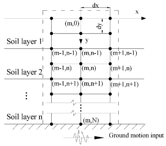
Figure 3.
Finite element discretization model of a horizontal layered soil layer.
When the SV wave or the P wave is incident perpendicularly, according to the propagation law of the wave in the medium, . The display method was used to solve Equation (4) as is shown in conference [27], and the acceleration and velocity terms were approximated by the finite difference method. The step value should meet the requirements stated in the conference [23]:
4. Free-Field Displacement Extension Solution
The relationship between the propagation velocity of waves in a medium and the horizontal apparent wave velocity is shown in Figure 4. If the medium is a horizontal layered medium, assuming the wave velocity of P wave or SV wave is c, Snell’s law [28] dictates that the horizontal apparent wave velocity , propagation velocity c, and incident angle of the incident wave are related as follows:
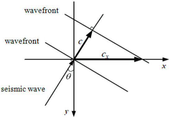
Figure 4.
Relationship between wave velocity and horizontal apparent wave velocity.
Figure 5 is the schematic diagram of the displacement expansion solution for the free wave field. After calculating the displacement of a column of nodes, the expansion can be solved according to the propagation law of the wave in the medium:
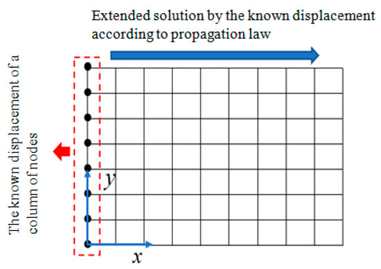
Figure 5.
Schematic diagram of the free-field displacement expansion solution.
When a P or SV wave is incident vertically, the horizontal apparent wave velocity is infinite (Equation (8)). According to Equation (9), the displacement of all boundary nodes and that of the nodes connected to the boundary nodes directly can be obtained. By substituting the solution into Equation (2), we can obtain the equivalent load on the boundary nodes. The above is the solution of the free-field two-dimensional plane model. For the three-dimensional model, the expansion solution can be obtained by using consistent displacement in the outward plane direction.
5. Near-Field Foundation-Bridge Model and Numerical Verification
In consideration of general vibration, research and testing using frequency domain methods can be achieved. But, considering the earthquake action, it is difficult to verify the test. It needs to be verified by shaking table test or large-scale test like centrifuge. This paper mainly proposes a numerical calculation method that simultaneously considers multi-point seismic and soil-dynamic interactions. And for the curved beam bridge, there is no test to verify it. The new method proposed in this paper is mainly compared with the extended numerical method that considers all the integral soil under the bridge. The results show that the method can achieve the accuracy of the extended numerical solution.
As shown in Figure 6, a pier model is located in a homogeneous semi-infinite space, regardless of the damping effect, and the pier parameters are shown. According to the characteristics of the soil-bridge structure system, a near-field foundation-bridge system model (right) shown in Figure 7 was established, and a direct solution model (left) was established for comparison to verify the model shown in Figure 7. In the direct solution model, a large space should be selected to eliminate the influence of the boundary, and the size of the selected soil region is 1000 × 1000 × 200 m. In the near-field foundation-structure system model, a small part of the soil area near the pier of dimensions 10 × 10 × 60 m was cut, and the equivalent viscoelastic artificial boundary element was introduced on the intercepting boundary. This is about 2 or 3 times by the dimension of the foundation.
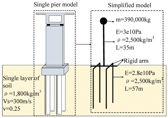
Figure 6.
Simplified model of the pier.
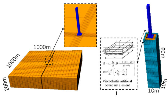
Figure 7.
Direct solution model (Left) and the substructure model (near-field.foundation-bridge model) (Right).
The displacement time history for input wave is shown in Figure 8. In the direct solution model, the horizontal displacement time history was applied at the bottom of the soil layer. In the substructure model, the input of ground motion was applied by transforming the displacement response of the intercepted area in the direct model into the equivalent load. The acceleration and displacement response time history at the media surfaces of the two models and those on the pier top are shown in Figure 9.
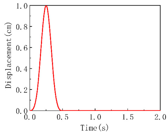
Figure 8.
Displacement loading function.
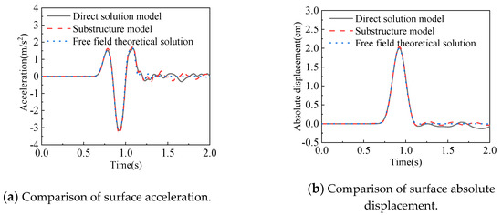
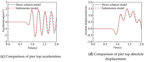
Figure 9.
Comparison of model responses.
Figure 9 compares the surface acceleration response and displacement response of the two models. The blue lines in (a) and (b) are the theoretical solutions of the free-field surface response of the without-pier model. The acceleration and displacement responses of the two models are highly fitted and are close to the free field theoretical solution of the without-pier structure. The impact of the pier on the free field response is negligible. Because of the kinematic interaction and the inertial interaction between the soil and foundation, the acceleration and displacement responses at the surfaces of the two models both oscillate after 1.17 s. Further, (c) and (d) show the acceleration and displacement response time history of the pier top, respectively. The results of the two models are very close. Therefore, the seismic response analysis based on the near-field foundation-bridge model is correct and has sufficient accuracy.
6. Synthesis of Multisupport-Related Ground Motion
Base on the near-field foundation-bridge numerical model, the coherence function is introduced to synthesize spatial multi-support related ground motion, considering nonuniform seismic action with spatial variation. This allows us to consider the influence of spatial variation of ground motion and the coherence effect between different foundations.
In this study, we chose the spatial coherence function model with anisotropic frequency as the independent variable [29]:
where X is the horizontal distance between i and j; is the circular frequency; is the shear wave velocity; and s is the coherence degree parameter. The larger the value, the higher is the degree of coherence, and the smaller the value, the lower is the coherence.
Based on the trigonometric series method, the correlated nonstationary ground motion time history of n points in space can be presented as the product of the stationary stochastic process and the nonstationary process envelope function [30]:
where , is the frequency step; N is the number of frequency points; is the upper cutoff frequency; , is the discrete frequency points; is the random phase angle uniformly distributed inside ; is the lower triangular matrix obtained by power spectral density matrix decomposition; and is the nonstationary strength envelope function for ground motion. The specific values of the parameters are taken in accordance with reference [30]. Baseline correction and filtering are performed after synthesizing the ground motions that satisfy certain error conditions to solve the baseline drift problem and removing spectral components unnecessary.
7. Analytical Method Based on the Separated Foundation Model
Based on the theoretical basis and numerical verification results, a seismic response analysis method for soil-curved beam bridge based on the separated foundation model was proposed. The method involves two parts: In the first part, the equivalent load of the simulated nonuniform ground motion field, which is implemented by MATLAB, is calculated. In the second part, the corresponding separated foundation finite element model is established. The specific process is shown in Figure 10.
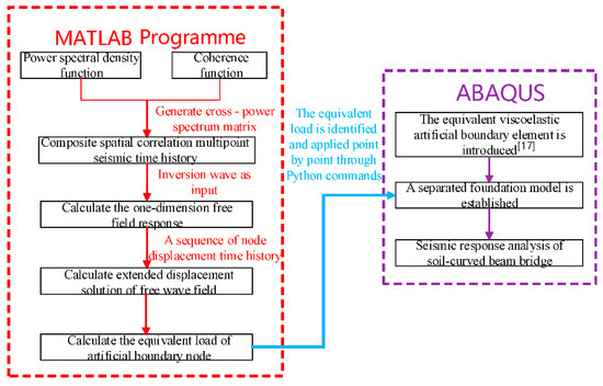
Figure 10.
Flow chart of the seismic response analysis.
8. Seismic Response Analysis of the Curved Beam Bridge
8.1. Project Overview
As shown in Figure 11, a typical curved beam bridge with a radius of curvature of 60 m and a span of m is taken as an example. The beam is box shaped with the top and bottom plates 8.75 m and 3.82 m wide, respectively, and its height is 2.12 m. The pier is rectangular, and its dimensions are . The height of piers P1–P5 is 35 m; and the pier has basin bearings to connect the upper and lower structures. Two fixed bearings are installed at piers P2–P4, and sliding bearings are installed at P1 and P5. All the piers are supported on the platform. The length of the pile is 57 m, and its diameter is 1.2 m. The foundation soil can be divided into four types: clay, silt, medium-coarse sand, and weakly differentiated fractured sandstone. The values of the soil parameters are shown in Figure 11. The beam concrete is C40; the pier is C30; the steel is HRB335 (); and the foundation pile is C25. The substructure layout and its dimensions of the bridge structure is the same as that of Figure 7.
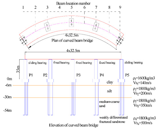
Figure 11.
Overall layout of the curved beam bridge.
8.2. Separated Foundation-Bridge System Finite Element Model
In order to consider the spatial variation effect of the ground motion, the foundation of the model was separated, and a separated foundation-bridge system model was established as shown in Figure 12. The curved beam bridge model and near-field soil were simulated by B31 beam element and solid element C3D8R in ABAQUS, respectively. For the pier, a uniaxial hysteresis model of concrete and steel materials was used based on implicit calculation [31]. The concrete constitutive was based on the Kent–Park model [32]. The ultimate stress was , and the corresponding ultimate strain was , ; Here, represents the volume-stirrup ratio; , the yield strength of the stirrup; and , the axial compressive strength. For the steel, a double-fold line model was used. The platform was modeled by a rigid body. The mass of the platform is added to the gravity center of it. The foundation piles were assumed as elastic and were simulated using elastic beam elements. The connection unit was used to simulate the connection between the beam and lower structure; the connection unit was assigned a proper hysteresis relationship. The yield force of the movable support was ; where , the sliding friction coefficient, was 0.02. The vertical force of the support was obtained by static analysis. The beam unit mesh of the area where the stress was concentrated near the beam and pier and the pier and platform was encrypted. The dimension of the separated foundation soil was 10 × 10 × 60 m, and that of the grid unit was 1 × 1 × 1 m. This is the same dimension as the one shown in Figure 7. The viscoelastic artificial boundary element was introduced at the same time [22]. The initial elastic modulus of the soil in the low strain state was , where is the ith layer density; is the ith layer shear wave velocity; and Rayleigh damping ().
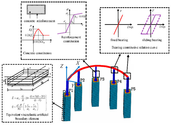
Figure 12.
Finite element model of the separated foundation-bridge system.
8.3. Generation of Seismic Coherent Waves
In order to study the influence of the spatial variation of ground motion on the seismic response of the curved beam bridge, the effects of different apparent wave velocities, degrees of coherence, and site conditions on the structural response were considered. Due to the limited space of the article, the theory of coherent wave generation is not fully described. But the basic flow can be obtained according to Figure 10. The ground motion needs to be synthesized according to the target spectrum. And after inversion of seismic waves, seismic acceleration and seismic velocity are obtained. Finally, the seismic velocity is used to obtain the time history force added to the model, which is used to simulate the seismic load.
According to the method described in Figure 10, four sets of displacement time histories of ground motions with different degrees of coherence were synthesized. Inversion waves were used as the input, and the displacement time histories of the inversion waves as obtained from the inversion of the soil layer parameters are shown in Figure 13. The wave passage effect was achieved by setting the time difference of the displacement time history curve of each point in advance. A total of 13 working conditions were considered, and the cases for different apparent wave velocities, degrees of coherence and site conditions are presented in Table 1. For the ground motion, two-way input was used, that is, in the axis direction of the string of the curved beam and the axis direction perpendicular to the string, the amplitude proportional coefficient of the input in the two directions was adjusted by 1:0.85 [33].
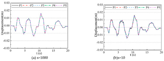
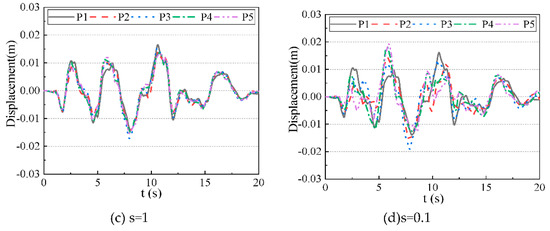
Figure 13.
Displacement time history of ground motion with different degrees of coherence.

Table 1.
Working conditions corresponding to different spatial parameters.
The maximum bending moment and torsion of the beam and the bending moment of the pier bottom under 13 different working conditions were considered according to the calculation results. The analysis of the effects of different ground motion parameters on the seismic response of the curved beam bridge is shown in Table 1.
8.4. Effect of Different Apparent Wave Velocities on the Structural Response
Figure 14 shows the magnitude of the seismic response—the internal force of the structure under working conditions 1–5. Compared with the situation under working condition 5 (apparent wave velocity is ), bending moment of the beam increased 0.67 times to 1.13 times; bending moment of the beam, 0.84 times to 5.26 times; the torsion of the beam, 0.74 times to 1.53 times; the tangential bending moment at the bottom of pier, 0.83 times to 1.32 times; and the radial bending moment, 0.84 times to 1.15 times.
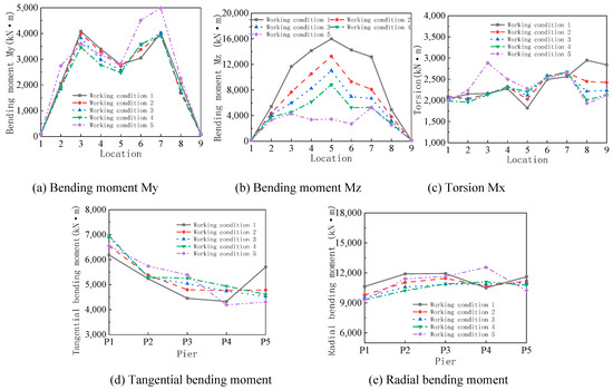
Figure 14.
Internal force responses of the beam and the bottom of the pier for different apparent wave velocities.
These results show that bending moment Mz of the beam is more sensitive to changes in the apparent wave velocity and that it increases as the apparent wave velocity decreases. Wave passage has little effect on the bending moment at the bottom of the pier.
8.5. Effect of Different Coherence on the Structural Response
Figure 15 shows the magnitude of the seismic response of the structure under working conditions 5–8. Compared with completely coherent working condition 5 (completely coherent), bending moment of the beam increased 0.62 times to 1.30 times; bending moment , 0.98 times to 7.15 times; the torsion of the beam, 1.08 times to 1.85 times; the tangential bending moment at the bottom of the pier, 0.68 times to 1.04 times; and the radial bending moment, 0.67 times to 1.18 times.
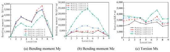
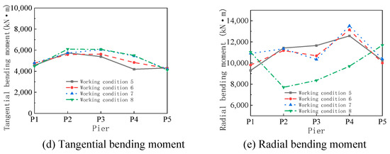
Figure 15.
Internal force response of the beam and the bottom of the pier under different values of coherence.
The results show that the incoherence has a great effect on bending moment response and the torsion response of the beam, and the structural response increases with the degree of incoherence. Bending moment of the beam decreases as the degree of incoherence increases. Incoherence has less effect on the bending moment at the bottom of the pier.
8.6. Effect of Different Site Conditions on the Structural Response
Figure 16 shows the magnitude of the seismic response of the structure under working conditions 9–13. Compared with working condition 11 (), bending moment of the beam increased 1.04 times to 2.81 times; bending moment , 1.01 times to 8.28 times; the torsion of the beam, 1.09 times to 3.03 times; the tangential bending moment at the bottom of the pier, 0.80 times to 1.47 times; and the radial bending moment, 1.02 times to 1.98 times.
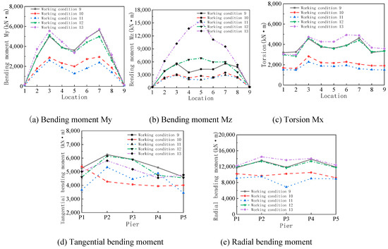
Figure 16.
Internal force response of the beam and the bottom of the pier under different site conditions.
The results show that the site conditions significantly change the magnitude of the seismic response of the structure. Overall, the worse the site conditions, the greater is the structural response. Bending moment of the beam is greatly affected when the stiffness of adjacent soil layers is different.
9. Conclusions
A new, feasible, and effective seismic response analysis method based on the separated foundation-curve-beam bridge model was proposed. This method employs the viscoelastic artificial boundary and wave input method in combination with the related ground motion synthesis method. The proposed method can reasonably consider the soil-structure interaction and the spatial variation effect of ground motion. It can be applied to the seismic response analysis of large bridges.
The seismic performance of curved beam bridges considering the soil-structure interaction was systematically analyzed. The effects of different apparent wave velocities, coherence, and site conditions were considered. The wave passage effect, effect of incoherence, and local site effect exert a large influence on bending moment and torsion when considering the soil-structure interaction. Soft soil sites have a greater impact on the bending moment at the bottom of the pier. Differences in the stiffness of adjacent soil layers have considerable influence on bending moment . Therefore, for small-radius curved beam bridges, the influence of spatial variation of ground motion should also be considered to avoid erroneous estimation of structural responses.
Author Contributions
L.Z. analyzed the data; Y.G. wrote the paper. All authors have read and agreed to the published version of the manuscript.
Funding
This research was funded by Ningxia Hui Autonomous Region Key R&D Projects (Grant No. 2018BDE02049) and General Program of National Natural Science Foundation of China (Grant No. 51578157).
Conflicts of Interest
The authors declare no conflicts of interest.
References
- Kahan, M.; Gibert, R.J.; Bard, P.Y. Influence of Seismic Waves Spatial Variability on Bridges: A Sensitivity Analysis. Earthq. Eng. Struct. Dyn. 1996, 25, 795–814. [Google Scholar] [CrossRef]
- Wang, D.; Sun, Z.; Li, X. Analysis of seismic damage and failure mechanism of curved beam bridge in Wenchuan earthquake. J. Disaster Prev. Mitig. Eng. 2010, 5, 572–579. [Google Scholar]
- Desroches, R.; Fenves, G.L. Evaluation of Recorded Earthquake Response of a Curved Highway Bridge. Earthq. Spectra 1997, 13, 363–386. [Google Scholar] [CrossRef]
- Chen, Y.; Wang, J.; Li, X. Random vibration analysis on A curved beam bridge Considering the Seismic Spatial Effect. Eng. Seism. Resist. Reinf. Transform. 2014, 36, 81–87. [Google Scholar]
- Sextos, A.; Kappos, A.J.; Mergos, P. Effect of Soil-Structure Interaction and Spatial Variability of Ground Motion on Irregular Bridges: The Case of the Krystallopigi Bridge. In Proceedings of the 13th World Conference on Earthquake Engineering, Vancouver, BC, Canada, 1–6 August 2004. [Google Scholar]
- Burdette, N.J.; Elnashai, A.S.; Lupoi, A.; Sextos, A.G. The Effect of Asynchronous Earthquake Motion on Complex Bridges. J. Bridge Eng. 2008, 23, 158–165. [Google Scholar] [CrossRef]
- Li, X.; Jia, H.; Li, Q. Experimental study on long-span curved rigid frame bridge under near-fault ground motion. J. Vib. Shock 2017, 36, 199–207, 237. [Google Scholar]
- Cheng, M.; Li, Q.; Yan, L. Experimental study on seismic response of irregular high-pier curved bridge under multi-point excitation. J. Vib. Eng. 2016, 5, 874–880. [Google Scholar]
- Bourouaiah, W.; Khalfallah, S.; Boudaa, S. Influence of the soil properties on the seismic response of structures. Int. J. Adv. Struct. Eng. 2019, 11, 309–319. [Google Scholar] [CrossRef]
- Zangeneh, A.; Battini, J.M.; Pacoste, C.; Karoumi, R. Fundamental modal properties of simply supported railway bridges considering soil-structure interaction effects. Soil Dyn. Earthq. Eng. 2019, 121, 212–218. [Google Scholar] [CrossRef]
- Khan, B.L.; Farooq, H.; Usman, M.; Butt, F.; Khan, A.Q.; Hanif, A. Effect of soil–structure interaction on a masonry structure under train-induced vibrations. Proc. Inst. Civ. Eng. Struct. Build. 2019, 172, 922–934. [Google Scholar] [CrossRef]
- Ramadan, O.M.O.; Mehanny, S.S.F.; Kotb, A.A.M. Assessment of seismic vulnerability of continuous bridges considering soil-structure interaction and wave passage effects. Eng. Struct. 2020, 206, 1–11. [Google Scholar] [CrossRef]
- Zain, M.; Usman, M.; Farooq, S.H.; Mehmood, T. Seismic vulnerability assessment of school buildings in seismic zone 4 of Pakistan. Adv. Civ. Eng. 2019, 14, 1–14. [Google Scholar] [CrossRef]
- Dai, G.; Liu, W.; Zeng, M. Research on ground motion response of urban viaduct curved beam bridge with small radius. Vib. Shock 2012, 31, 155–160. [Google Scholar]
- Sextos, A.G.; Taskari, O.; Manolis, G.D. Influence of Seismic Wave Angle of Incidence Over the Response of Long Curved Bridges Considering Soil-Structure Interaction. In Dynamic Response of Infrastructure to Environmentally Induced Loads; Springer: Berlin, Germany, 2017. [Google Scholar]
- Ye, A.; He, J. Seismic response analysis method of cable-stayed bridge based on integrated model. J. Tongji Univ. (Nat. Sci.) 2013, 41, 1326–1332. [Google Scholar]
- Cairo, R.; Francese, G.; Moraca, R.; Aloe, F. Seismic Soil-Pile-Structure Interaction. Theoretical Results and Observations on Pile Group Effects. In CNRIG 2019: Geotechnical Research for Land Protection and Development; Springer: Berlin, Germany, 2020. [Google Scholar]
- Papadopoulos, S.; Sextos, A.; Kwon, O. Impact of spatial variability of earthquake ground motion on seismic demand to natural gas transmission pipelines. In Proceedings of the 16th World Conference on Earthquake, Santiago, Chile, 9–13 January 2017. [Google Scholar]
- Liu, J.; Tan, H.; Bao, X. Seismic wave input method based on artificial boundary substructure in soil-structure dynamic interaction analysis. Chin. J. Theor. Appl. Mech. 2018, 50, 32–43. [Google Scholar] [CrossRef]
- Hao, H. Effects of Spatial Variations of Ground Motion on Large Multiple-Supported Structures; Earthquake Engineering Research Center, University of California at Berkeley: Berkeley, CA, USA, 1989. [Google Scholar]
- Shinozuka, M.; Deodatis, G. Effect of Spatial Variation of Earthquake Ground Motion on Seismic Response of Bridges; Technical Report; NCEER: Burlingame, CA, USA, 1997. [Google Scholar]
- Gu, Y.; Liu, J.; Du, Y. Three-dimensional uniform viscoelastic artificial boundary and equivalent viscoelastic boundary element. Eng. Mech. 2007, 24, 31–37. [Google Scholar]
- Liu, J.; Wang, Y. One-dimensional time domain algorithm for in-plane free wave field in layered media. Eng. Mech. 2007, 24, 16–22. [Google Scholar]
- Liao, Z. Finite element method for near-field fluctuation problem. Earthq. Eng. Eng. Vib. 1984, 2, 3–16. [Google Scholar]
- Zhou, G.; Bao, Y.; Li, X.; Peng, X.B. Review of multi-point excitation problems in structural dynamic analysis. World Earthq. Eng. 2009, 25, 25–32. [Google Scholar]
- Huang, B.; Shen, W.; Lu, Z. Influence of Rayleigh damping on large-mass direct integration time history calculation method. Nucl. Power Eng. 2015, 2, 21–23. [Google Scholar]
- Zhuo, W.; Gao, Z.; Gu, Y. One-dimensional time-domain algorithm for free wave field of damped layered media when P-SV wave is obliquely incident. J. Water Resour. Archit. Eng. 2016, 14, 18–24. [Google Scholar]
- Li, Z.; Liu, D. Waves in Solid; Beijing Science Press: Beijing, China, 1995. [Google Scholar]
- Vanmarke, E.H. Conditional simulation of spatially correlated ground motion. J. Eng. Mech. 1993, 119, 2333–2352. [Google Scholar] [CrossRef]
- Novak, M.Š.; Lazarević, D.; Atalić, J. Influence of spatial variability of ground motion on seismic response of bridges. Građevinar Časopis Hrvatskog Saveza Građevinskih Inženjera 2015, 67, 943–957. [Google Scholar]
- Pan, P.; Qu, Z.; Xiao, M.; Zhou, F.; Ye, L.P. Elastoplastic time history analysis of reinforced concrete structures based on ABAQUS. In Proceedings of the Academic Seminar on Collapse Resistance of Building Structures, Beijing, China, 5 June 2010. [Google Scholar]
- Scott, B.D.; Park, R.; Priestley, M.J.N. Stress-strain behavior of concrete confined by overlapping hoops at low and high strain rates. ACI J. 1982, 79, 13–27. [Google Scholar]
- GB50011-2010. Code for Seismic Design of Buildings; National Standard of the People’s Republic of China: Beijing, China, 2010. (In Chinese) [Google Scholar]


© 2020 by the authors. Licensee MDPI, Basel, Switzerland. This article is an open access article distributed under the terms and conditions of the Creative Commons Attribution (CC BY) license (http://creativecommons.org/licenses/by/4.0/).