Abstract
Deep learning based intelligent fault diagnosis methods have become a research hotspot in the fields of fault diagnosis and the health management of rolling bearings in recent years. To effectively identify incipient faults in rotating machinery, this paper proposes a novel hybrid intelligent fault diagnosis framework based on a convolutional neural network and support vector machine (SVM). First, an improved one-dimensional convolutional neural network (1DCNN) was adopted to extract fault features, and the state information and intrinsic properties of the raw vibration signals were mined. Second, the extracted features were used to train the SVM, which was applied to classify the fault category. The proposed hybrid framework combined the excellent classification performance of the SVM for small samples and the strong feature-learning ability of CNN network. In order to tune the parameters of the SVM, an improved novel particle swarm optimization algorithm (INPSO) which combined the Tent map and Lévy flight strategy was proposed. Numerical experimental results indicated that the proposed PSO variant had a better performance in searching accuracy and convergence speed. At last, multiple groups of rolling bearing fault diagnosis experiments were carried out and experimental results showed that, with the proposed 1DCNN-INPSO-SVM model, the hybrid framework was capable of diagnosing with high precision for rolling bearings and superior to some traditional fault diagnosis methods.
1. Introduction
Rotating machinery plays an important part in modern industrial manufacture, and its failure may cause unpredictable security accidents and economic losses [1]. Therefore, the identification and diagnosis of rotating machine faults is one of the major topics in the study of mechanical systems fault prevention [1,2]. Rolling element bearings are considered to be the key components in a rotating mechanism system, and faults occurring in the rolling element bearings can not only have a direct and massive influence on the stability of the system, but also shorten the service life of the machine [3]. Therefore, after the vibration signals are collected from the sensors, the most effective way for the rolling bearings to avoid possible damage is to establish a highly efficient and intelligent fault diagnosis and health monitoring system [4]. Generally, intelligent fault diagnosis methods can be divided into two steps, namely feature extraction based on signal processing and health status recognition based on the classification model [5]. The raw signals collected from multiple sensors contain useful information about the running status of the machine, as well as useless noises in the time domain. Therefore, it is necessary to find an effective feature extraction method to obtain intrinsic features of the signals. Wavelet packet transformation (WPT) [6], empirical mode decomposition (EMD) [7] and fast Fourier transformation (FFT) [8] are three kinds of widely applied feature extraction methods in the vibration signal processing field. After feature extraction, principal component analysis (PCA) [9] and independent component analysis (ICA) [10] methods usually are selected to remove the low sensitivity and useless data from the extracted features. With the feature vectors selected and extracted from raw signals, state classification is accomplished by K nearest neighbor (KNN) [11], support vector machine (SVM) [12] and other machine learning algorithms and statistical frameworks [13,14]. The application of traditional fault diagnosis algorithms has achieved certain results, but there are still some shortcomings, such as the feature selection excessively relies on the experience and prior knowledge of the engineers [15], furthermore, it is very subjective and time-consuming [16]. At the same time, traditional machine learning models are faced with dimensional disaster, overfitting and other problems, and the shallow models are difficult to represent the complex mapping relationships between signal samples and health status [17].
As Hinton et al. [18] proposed the method of layer-by-layer unsupervised training combined with supervised fine-tuning, deep learning (DL) theory has become a great breakthrough in the field of machine learning and artificial intelligence [16]. Compared with traditional intelligent fault diagnosis methods, the deep model can learn representative invariable features and complex nonlinear relationships from the raw data automatically. As a classical deep learning model, the convolutional neural network (CNN) has a strong feature learning ability with its unique convolution structure, which has achieved great success in the field of image recognition and has been widely applied in fault diagnosis. Chen et al. [19] proposed a CNN model used for intelligent fault diagnosis of gearboxes with manually extracted features. Wang et al. [20] proposed a CNN model for rotating machinery conditions recognition whose inputs are two-dimensional matrix transformed by time domain signals. Janssens et al. [21] adopted the data processed by the discrete Fourier transform method as the inputs of a three-layer CNN model for fault diagnosis. Many research results show that the CNN network has a strong ability for learning sensitivity and robustness. However, how to preprocess the raw data efficiently, e.g., the transformation process of one-dimensional vibration signals into two-dimensional matrices for CNN inputs, is a thought-provoking question. To the best of our knowledge there is no complete theory to guarantee the transformation is reasonable. In this paper, the proposed 1DCNN network avoids time-consuming data preprocessing and extracts features more accurately by carrying out automatic adaptive learning on one-dimensional raw vibration signals. In the field of image processing, the fully connected layer of a CNN network generally adopts softmax function to classify, which can achieve a good classification accuracy. However, for fault diagnosis problems, the training data volume is much smaller than that of the image processing, which means that the depth model is difficult to obtain ideal results in dealing with fault diagnosis problems independently. For SVM, the idea of kernel function is adopted to map nonlinear samples to a high-dimensional space and make it linearly separable, and then SVM finds an optimal hyperplane that maximizes the classification interval between data sets, thus promoting classification performance [22]. Many research works have proved that the SVM has a strong learning ability for small sample classification problems. Therefore, by combining 1DCNN with the SVM, the extracted sparse representative feature vectors from the second fully connected layer of the network are taken as the inputs of the SVM for achieving optimal classification accuracy. However, the standard SVM needs to preset two crucial parameters (i.e., penalty factor c and kernel parameter g), which have a great influence on its classification performance [23]. To solve this problem, various optimization methods are applied to tune SVM parameters, such as genetic algorithm (GA) [24] and particle swarm optimization (PSO) [23]. Recently, the particle swarm optimization algorithm has achieved remarkable results in many works. However, the original PSO algorithm has some drawbacks, e.g., premature and slow convergence speed. To avoid those shortcomings, this paper proposed an improved novel particle swarm optimization algorithm (INPSO) for SVM parameter optimization.
In this paper, we propose a novel fault diagnosis method based on the one-dimensional convolution neural network (1DCNN) and SVM optimized by INPSO (INPSO-SVM) to improve diagnosis accuracy. To sum up, there are three main contributions existing in the proposed method. Firstly, the proposed method directly extracts the features of the original time-domain vibration signals by applying a 1DCNN network, without any time-frequency conversion. Secondly, the excellent small sample learning abilities of the SVM is combined with the powerful deep feature adaptive learning ability of 1DCNN to improve the diagnosis accuracy. Finally, an improved particle swarm optimizer variant is presented to tune the parameters of SVM, which can improve the classification accuracy and generalization performance of SVM. The engineering application and contrastive tests reveal the effectiveness and superiority of the proposed method.
The remainder of this paper is organized as follows: Section 2 is dedicated to the basic knowledge of CNN, SVM, and PSO. Section 3 introduces the proposed fault diagnosis method based on 1DCNN model and INPSO optimized SVM. Section 4 discusses the results of the experiments. The conclusion is summarized in Section 5.
2. Fundamental Theories
2.1. Convolutional Neural Network
CNN is a typical feed-forward neural network model which is composed by a trainable feature extraction part and a classification part [16,25]. The feature extraction part mainly includes convolutional layers and pooling layers [21], and the classification part is a multilayer perceptron consisting of several fully connected layers [26].
In the convolutional layers, the input samples are convolved with a bunch of learnable convolution kernels to extract feature vectors [16]. Usually a convolution layer has multiple convolution kernels and a class of features learned from a convolution kernel are called mapping graphs. The operation can be expressed as follows.
where donates the convolution operator, i donates the layer number of the network, k is the index of the output feature maps, is the input feature map of j-th local region, and is the k-th output feature map after the convolution calculation. and are the weight and the bias of the k-th group filter in the i-th layer.
In recent years, the rectified linear unit (ReLU) has been widely used as an activation element to accelerate the convergence of neural networks [26]. ReLU model can be described by Equation (2).
where is the output value of the convolution operation, is the activation of .
A pooling operation is adopted to reduce the computational complexity, and effectively control the risk of overfitting [27]. Max-pooling is defined as follows.
where denotes the value of t-th neuron in the k-th output feature map of the i-th layer. is the pooling length, and is the output feature map after the pooling operation.
In a traditional convolutional neural network, after several convolutional layers and pooling layers, the feature maps learned by each kernel function are flattened into a one-dimensional array as the input of the fully connected layer. The output of the fully connected layer is a one-dimensional vector, and the mathematical model of the fully connected layer is described as follows.
where is the activation function, is the input of a fully connected layer, denotes the output of a fully connected layer, and w, b are the bias and the weight.
2.2. SVM Classifier Parameters Tuning
2.2.1. Support Vector Machine
A SVM is a widely used machine learning method based on the minimization principle of structural risk [23]. It has many unique advantages in solving small sample, multi-class, non-linear and high-dimensional pattern recognition problems [5]. In this paper, the proposed method mainly uses a nonlinear multi-class SVM as the backend multi-class classifier to solve the classification problem [28]. Given a group of sample set , where presents the N dimensional input feature of the i-sample, and is the corresponding label for the input sample. If the hyperplane equation reaches the criterion of the optimal separating plane, the optimal separation plane can be solved by the following objective functions and constraints.
where denotes the weight vector and depicts the bias vector, is the relaxing factor and c is a constant named as the penalty factor and it can relieve contradiction between algorithm complexity and classification accuracy. Finally, the classification problem of SVM are transformed to the following dual optimization problem.
where are the Lagrangian multipliers, and represents a kernel function that meets , where the is the inner product operation. The final SVM classification function is:
2.2.2. Particle Swarm Optimization Algorithm
In the original PSO algorithm, there are N particles in the population, and each particle i has a position vector and a velocity vector to calculate its current state, where D is the dimensions of the solution space. First, the initial positions and velocities of the particles are randomly initialized in the search area, where the position of each particle represents a solution. The fitness value can be calculated by substituting the vector into the target function. Then by comparing the fitness value of each particle, the position with the best fitness value is the optimal position of the current population. At last, in the t + 1 iteration of the particle, the positions and velocities of the particles are updated according to Equations (8) and (9).
where is inertia weight to control the impact of the previous velocity. are the learning factors, and are random numbers in [0, 1] for denoting remembrance ability. represent the g-th generation velocity and position of the i-th particle respectively, is the optimal position that the i-th particle has searched so far, and is the historical optimal value searched by the whole population.
3. Fault Diagnosis Method Based on 1DCNN and INPSO-SVM
3.1. Overall Framework of the Proposed Method
To improve the fault diagnosis accuracy of rolling bearings, a novel hybrid fault diagnosis scheme which combines the 1DCNN and INPSO-SVM is proposed in this paper. Figure 1 shows the flowchart of the proposed method, which can be divided into three major steps (i.e., data collection, feature extraction and fault classification). The raw fault data from multiple sensors is directly input into the improved 1DCNN model for the training of a CNN model. The outputs of the fully connected layer are taken as the feature vectors which are input into the SVM classifier for fault classification. Since the classification performance of an SVM classifier is susceptible to the values of parameters c and g, the proposed INPSO is adopted to tune the parameters of the SVM.
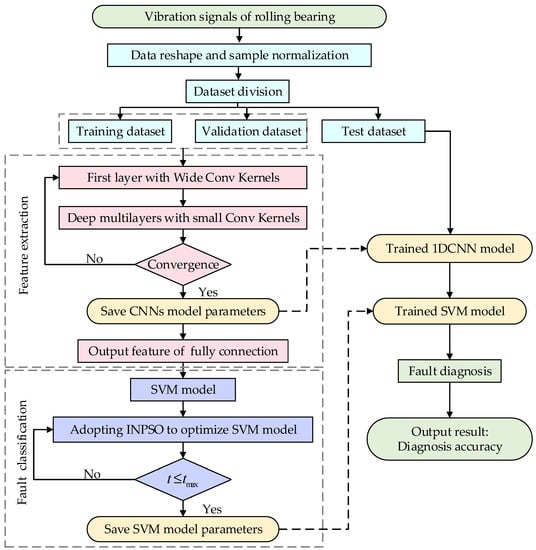
Figure 1.
The framework of the proposed one-dimensional convolutional neural network improved novel particle swarm optimization support vector machine (1DCNN-INPSO-SVM) intelligent fault diagnosis method.
3.2. Feature Extraction Based on 1DCNN
The training process of the convolutional neural network can be divided into a forward propagation stage and a backward propagation stage. In the process of forward propagation, the network firstly initializes the weights, and then convolution kernels filter each small region of the data to obtain the eigenvalues of the small region. The features obtained from the convolution layer are passed into the lower sampling layer, where the dimension and quantity of trainable parameters are reduced to avoid overfitting by pooling. Finally, the features extracted from the lower sampling layer are transferred to the fully connected layer and the softmax layer for classification, and the classification model is obtained to get the final fault diagnosis results. When the output results of the convolutional neural network are inconsistent with the real labels, the errors are propagated from the high level to the low level in the backward propagation stage. According to the ratio of each layer of errors to the total errors, the weights of each layer are updated. In the training stage of CNN, dropout technology, data sliding window expansion technology and batch normalization technology are used to prevent over-fitting and speed up the training process. The structure of the proposed 1DCNN network is shown in Figure 2.

Figure 2.
Structure of the proposed 1DCNN model.
The overall structure of proposed 1DCNN network is composed of four convolution layers, four maximum pooling layers and two fully connected layers. Details about the architecture of 1DCNN can be found in Table 1. The input signals are the normalized time-domain signals. Features can be extracted directly from the raw time domain signals by using one-dimensional convolution kernel and pooling kernel, which reduces the work of signal preprocessing. Compared with traditional CNN structure, the main advantage is that the convolution kernel of the first layer is larger in size to better suppress the high-frequency noise, and the following convolutional kernels are small with 3 × 1, which is helpful to obtain a good representation of the input signals and improve the network performance.

Table 1.
Parameters of 1DCNN algorithm applied in the experiments.
3.3. Fault Identification Based on INPSO-SVM Algorithm
A support vector machine (SVM) is an efficient machine learning tool developed by Vapnik [29], but the penalty factor c and kernel parameter g of a SVM classifier mainly rely on manual selection, which has a great impact on the recognition accuracy of the SVM classifier. In general, the penalty factor c represents the nonlinear fitting ability. If the parameter c is extremely large, SVM will lose the generalization ability [23]. The size of the kernel parameter g affects the kernel mapping distribution of the data samples. Therefore, parameter tuning is essential for the SVM to get a good classification performance. In view of this, an improved new PSO variant is proposed to optimize the SVM parameters in this study.
3.3.1. An Improved New PSO Algorithm (INPSO)
In order to overcome the problem of trapping into local minimums and facilitate the convergence speed of the basic PSO algorithm, a novel population initialization method based on Tent map and an enhanced particle position update approach based on Lévy flights was developed. The modified method can reduce the population degradation and enrich the population diversity. Moreover, the premature convergence is avoided by searching the neighborhood of the particles that have fallen into local optimums.
Chaos Based Initialization
In the standard PSO algorithm, the initial positions of the particles are initialized randomly, which affects the search efficiency of the algorithm and limits the optimization ability of the PSO algorithm. Since the 1990s, with the study of chaos theory, chaotic maps have been widely applied in various fields. Chaos is a typical nonlinear phenomenon in nature, a chaotic system can go through every state in a certain range without repeating according to its own rules. Adding chaos operator into the optimization algorithm can improve the global search ability of the algorithm [30]. Among the chaotic systems, the structure of Tent map is simple, and its ergodic performance produces uniform distribution chaotic sequences, and the iteration process is suitable for computer operation [31]. The mathematical model of Tent chaos map is defined as follows.
where, N is the population size, and rand (0, 1) is a random number within the range of (0, 1). The introduction of random variable not only ensures the randomness, ergodicity and regularity of the Tent chaotic map, but also effectively avoids iterations falling into the points of small period and unstable period.
An Enhanced Particle Position Updating Strategy
Lévy flight, proposed by Paul Lévy, is a non-gaussian random process [32]. The short distance walk of Lévy flight mechanism improves the diversity of the population, and the directional variability of the occasional long jump ensures that the population searches the surrounding area in detail. The combination of a short distance walk and a long distance jump can fully search the solution domain and greatly improve the global optimization ability of the algorithm.
In the proposed INPSO algorithm, this paper eliminates the influence of the velocity term, and the particle swarm position is updated by the following equation.
where, is a random particle in the current set of particles, represents the learning factor of random particle, is drawn from the uniform distribution range in [0, 1]. The fourth term is a random learning mechanism, which can increase the diversity of the population and overcome premature convergence.
In order to make a good balance between local and global search capability, the particle swarm optimization algorithm is combined with an improved Lévy flight strategy to obtain a new generation of particle swarm. The updating equation of group position is defined by Equation (12).
where, is random step size, represents the dot product, is a random search path that conforms to Lévy distribution and meets the following constraints [33].
where, follow a standard normal distribution, = 1.5, and is defined as follows.
Combined with the improved Lévy flight, the new algorithm has a better coordination between exploratory and exploitative patterns. At the same time, the greedy selection is added into the algorithm, which helps the PSO to only preserve the better-quality solutions with regard to the fitness values. The implementation of this process is described as follows.
The specific implementation steps of the proposed INPSO algorithm are presented as follows:
Step 1: Set the size of the population to N, dimension D, maximum number of iterations and initialize the values.
Step 2: Initialize population using Tent mapping defined by Equation (10).
Step 3: Calculate the individual fitness value .
Step 4: Select the global and local optimal solution.
Step 5: Use Equation (12) to update the location of particles, then recalculate the fitness values and update the values of the particles.
Step 6: Select the particles according to the greed principle described by Equation (15).
Step 7: Judge whether t reaches value, if reached, the fitness value of α is output, that is, the best solution. Else go to Step 3.
3.3.2. Optimization of SVM Parameters Based on INPSO
The position coordinates corresponding to the optimal solution of the particle swarm are the best values of SVM parameters c and g. The flow chart of the SVM parameters tuning process based on INPSO is illustrated in Figure 3.
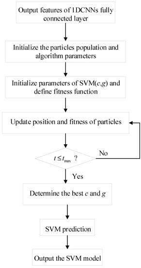
Figure 3.
INPSO-SVM flow chart.
4. Validation of the Proposed Method
4.1. INPSO Algorithm for Numerical Function Optimization
In order to strictly investigate the capabilities of the INPSO, eight classical benchmark functions were selected for simulation. The equations of selected functions and their brief descriptions are provided in Table 2, where are the unimodal benchmark functions, and are the multimodal functions. To substantiate the efficiency of INPSO, the SCA, CS and PSO were utilized to optimize these benchmark tasks and the experimental results were compared with those obtained by INPSO. For fair comparisons, the common parameter settings of the four algorithms were the same: population size N = 30, dimensions d = 30 and the maximum number of iterations was 500. For SCA, the parameters were set to be: a = 1, and were random numbers. The parameters of CS were set to be pa = 0.25. For PSO, the parameters were set to be: , , and . Then we separately simulated 30 times and recorded the average values and standard deviations. The average values of the experiments were used to reflect the convergence accuracy and speed of the algorithms with a given number of iterations. The standard deviations were used to reflect the stability of the algorithms. The results are shown in Table 3.
Table 2.
Benchmark functions.
Table 3.
Optimization results on unimodal and multimodal functions.
To further illustrate the optimization performance of the proposed INPSO, the convergence curves are exhibited in Figure 4. The curves shown in these figures were the average fitness values achieved from 30 independent experiments. As can be seen from Table 3 and Figure 4, in terms of , the INPSO algorithm was superior to the other algorithms and could obtain solutions quite close to the global optimums. The solution accuracy of function even reached the level of 5.97 × 10−63, which showed that the algorithm had obvious superiorities and made up for the deficiencies of the basic PSO algorithm. On two multimodal functions ( and ), though the INPSO algorithm could not get the minimum standard deviations under the specified maximum number of iterations, the best and mean of the objective values performed better than the other four algorithms. For the convergence curves of and , its convergence speed was obviously faster than the other three algorithms during the initial stage, and the curves showed that the INPSO algorithm could reveal a promising exploitation potential. To sum up, all simulation results indicated that the proposed INPSO had better performances in search accuracy and speed.
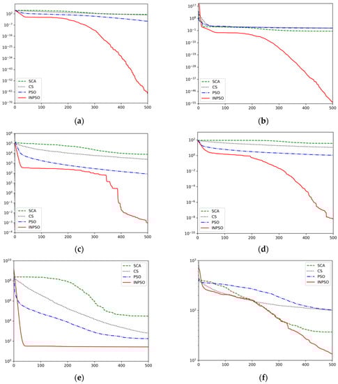
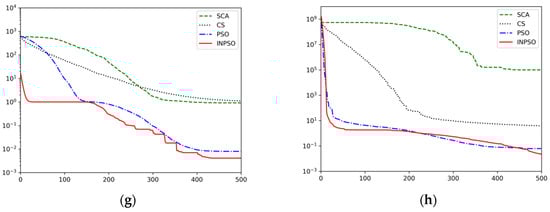
Figure 4.
Convergence trends for INPSO versus other optimizers: (a) Sphere function, (b) Schwefel 2.22 function, (c) Schwefel 1.2 function, (d) Schwefel 2.21 function, (e) Rosenbrock function, (f) Rastrigin function, (g) Griewank function, (h) penalized function.
4.2. Case 1: Experiment Results on the CWRU Bearing Dataset and Performance Analysis
4.2.1. Data Collection
In this section, vibration signals of different fault states collected by the motor experimental bench of Case Western Reserve University [34] were used as experimental data to verify the effectiveness of the proposed method in rolling bearings fault diagnosis. As shown in Figure 5, the experimental platform mainly consisted of a torque transducer, a load motor and a three-phase induction motor. In the test, vibration signals collected from the drive end (DE) were treated as the research target, where the sample frequency was 12 kHz and the rotation speed was 1730 r/min under the rated load of 3 hp. The experimental device adopted electric spark machining technology to simulate three fault states of rolling bearings: ball fault, inner race fault and out race fault, and the depth of the faults was 0.011 inches. Each fault state included three degrees of fault with width of 0.007 inch, 0.014 inch and 0.021 inch, respectively.
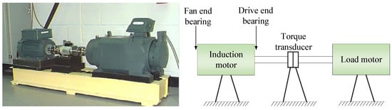
Figure 5.
The rolling bearing fault data acquisition experimental bench.
In this experiment, the data set contained 1000 groups of training data, and each training sample contains 864 sampling points. The standardized fault samples under each fault state were randomly divided into training data set and test data set with the scale of 7:3. Since different fault diameters at the same position were regarded as different fault types, so there were ten categories of health conditions in total. We selected the same amount of data under each operating condition, 70 samples were used as the training set and 30 samples were used as the test set. In this way, this method ensured the balance of data and facilitated the diagnosis model to get correct diagnosis results.
4.2.2. 1DCNN Feature Learning Verification and Analysis
In order to demonstrate the superiority of the proposed 1DCNN feature learning method, three other mainstream feature extraction methods, including wavelet packet transform (WPT), convolutional auto-encoder (CAE) and long short-term memory (LSTM), were applied to extract feature vectors for comparison using the same fault dataset. Firstly, the feature extractions of the raw vibration signals were conducted using the above four feature extraction methods. Then the SVM was adopted as the classifier to accomplish the fault classification task. To avoid randomicity, the grid search method and 3-fold cross validation were adopted for the parameter optimization of SVM, and the parameters c and g were set in the ranges of [0.001, 0.1] and [1, 100], respectively.
The main parameters of the other methods are briefly described as follows: (1) WPT: the energy spectra were calculated after the vibration signals were decomposed by three-layer wavelet packet decomposition. (2) CAE: using two layers of the convolutional layer, two layers of the pooling layer and two layers of the full-connected layer. The convolutional kernels were 64 × 1 and 8 × 1, the length of each pooling layer was 2, the Adam optimization algorithm was used and the activation function was ReLu. (3) LSTM: the model consisted of two LSTM layers, two fully connected layers, and one softmax layer. The dropout rate was 0.2, the batch size was 128, and the iteration epoch was 30.
As the dataset and the classifier used in the contrast experiments were the same, the differences in fault diagnosis performance were totally caused by the fault extraction processes. The precision rates and the recall rates of the four methods (i.e., 1DCNN-SVM, WPT-SVM, CAE-SVM and LSTM-SVM) are summarized in Table 4. To illustrate the differences more directly, F1-measure values (percentage form) of the four methods are presented in Figure 6.
Table 4.
The precision rate and recall rate of different methods.
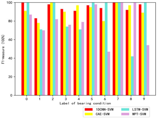
Figure 6.
The F1-measures of the bearing data using different methods.
From Table 4 and Figure 6, it can be observed that the average precision rate of SVM with manual feature extraction (WPT) was only 80.8%, while the deep learning models (LSTM-SVM, CAE-SVM) had better performances (about 10% improvement in precision rate) compared with traditional WPT feature extraction method. The 1DCNN-SVM model achieved the best average precision rate (95%) using a four-layer convolutional neural network. The accuracy of the proposed 1DCNN-SVM algorithm was obviously better than other competitors, which meant that the 1DCNN had advantages in feature learning of vibration signals compared with other intelligent feature extraction methods, e.g., CAE, LSTM. All four algorithms had high diagnosis accuracies for the normal state (condition 0), however the performance of 1DCNN-SVM algorithm was significantly better than those of the other three algorithms for the micro-fault identifications (condition 1 and condition 3). In summary, compared with WPT-SVM, CAE-SVM, and LSTM-SVM, the 1DCNN-SVM algorithm had a more superior overall performance both in diagnosis accuracy and stability, which indicated that 1DCNN was a more promising feature extraction tool for rolling bearings fault diagnosis. In addition, 1DCNN could extract the features of the raw vibration signals directly without a complicated signal preprocessing process, which had advantages over traditional methods.
Generally, the CNN was considered as a black box, and its inner working mechanism was difficult to understand [35]. In this paper, we tried to explore the internal operation process of the proposed 1DCNN model with a visual method. In order to explore the network feature extraction ability of each layer of 1DCNN, a t-Distributed Stochastic Neighbor Embedding(t-SNE) method was adopted in this paper to visualize the outputs of each network layer by mapping the high-dimensional feature vectors into three-dimensional space, and the data feature distributions of each layer after dimension reduction are shown in Figure 7. Figure 7a indicates that the original data sampled under 10 running states were overlapped seriously. However, it can be seen clearly from Figure 7b–f that the data sampled under different fault conditions were gradually separated due to the feature extraction ability of each layer being gradually enhanced. Finally, after the fully connected layer, the final obtained features were easily distinguishable which meant that the 1DCNN network had a good feature learning capability.
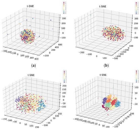
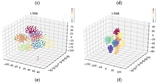
Figure 7.
Scatter plots of the feature visualization by t-SNE: (a) feature distribution of raw data, (b) feature distribution of convolutional layer 1, (c) feature distribution of convolutional layer 2, (d) feature distribution of convolutional layer 3, (e) feature distribution of convolutional layer 4, and (f) feature distribution of the fully connected layer.
4.2.3. Bearing Fault Diagnosis Experiment
Fault Diagnosis Results and Evaluation of the Proposed INPSO Optimization Method
During the optimization stage, the proposed INPSO approach was used to optimize the penalty factor c and the kernel parameter g, where the number of particles was set to 20, the number of iterations was 100, and the search ranges of c and g were set to [0.001,10]. Fitness values were calculated by threefold cross validation for the training samples. A group of samples was randomly selected as the test set, and the proposed 1DCNN was applied for feature extraction. The extracted feature vectors were respectively fed into three classifiers (SVM, PSO-SVM and INPSO-SVM), where the parameter settings of the PSO and INPSO algorithms were the same. Each method was performed 10 times and the diagnosis accuracy of three classifiers are listed in Table 5. As can be seen from Table 5, in the standard SVM, the default parameters c and g of SVM respectively were 1 and , where n was the data dimension. The fault diagnosis accuracy of the test set was 93.6% without the parameters tuning process of SVM. As a contrast, the PSO algorithm was used to optimize SVM parameters, and the average fault diagnosis accuracy of PSO-SVM was 90.56% with a standard deviation of 10.52. This means that the diagnosis accuracy was not stable and the parameter optimization process of the PSO was easily trapping into local optimums. In order to further evaluate the effectiveness of the proposed INPSO method, with the same test set, SVM optimized by INPSO was applied to do fault diagnosis experiments and the experimental results revealed that the average accuracy of the test set could reach 96.97%, and the standard deviation was only 0.69. Therefore, we could conclude that the diagnosis accuracy and robustness of INPSO-SVM was better than PSO-SVM and SVM method, which meant that the proposed INPSO overcame the shortcomings of original PSO, e.g., trapping into local optimums, and had a stronger global optimization ability.
Table 5.
The accuracy of different fault diagnosis methods.
Figure 8 and Figure 9 depict the convergence curves of INPSO algorithm compared with the original PSO algorithm in the first trial. The optimal fitness value of PSO and INPSO algorithm in the first iteration were both 70.72%. With the progress of iteration, the accuracies of the SVM optimized by two algorithms rose rapidly, while the particles fell into local optimums in the second iteration. At this point, the fitness achieved 80.87%. After a couple of iterations, the optimal fitness value of PSO algorithm did not change, while Lévy flight helped the particles jump out of the local optimums and find a better global solution in the proposed INPSO algorithm. The accuracy of the proposed INPSO-SVM method was higher than that of the PSO-SVM, reaching up to 100.0% in the training process. The training results also showed that the proposed INPSO approach had a better performance in the parameters tuning process and INPSO-SVM achieved a higher diagnosis accuracy.
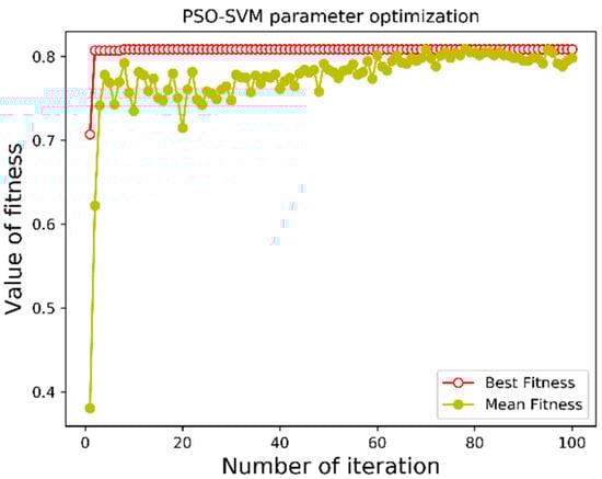
Figure 8.
Diagnosis accuracy of PSO-SVM algorithm.
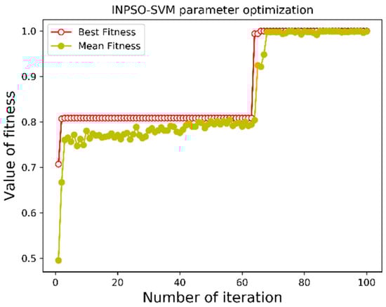
Figure 9.
Diagnosis accuracy of INPSO-SVM algorithm.
Comparisons Among Different Fault Diagnosis Methods
In this subsection, comparative studies between the WPT-INPSO-SVM and the proposed 1DCNN-INPSO-SVM were performed to verify the effectiveness and superiorities of the proposed algorithm. In the comparative experiments, there were three points that need to be emphasized. Firstly, the 8-dimensional vectors extracted by the three-layer wavelet packet were used as the inputs of the INPSO-SVM classifier for fault diagnosis, and the parameters of the proposed INPSO algorithm were consistent in the contrast experiments. Secondly, for the fault diagnosis comparison test, two algorithms processed the same ten group of data (A-J) which were randomly selected from the original signal. Thirdly, the average values of the two models were taken as the final experimental results after 10 trials for each group of data, where particles iterated 100 times to find the optimal value. Diagnosis results are listed in Table 6. There were some identical recognition results, such as the 80% accuracy for the first set of data. Because the raw data used in the ten experiments were the same, and WPT used the same three-layer wavelet packet to extract 8-dimensional feature vectors, which meant that the extracted features by WPT were the same in the ten times of experiments. In addition, the INPSO algorithm might find the same optimal parameter values for SVM. Therefore, the raw data, the extracted features and the models of classifiers were all the same in this case, and the experimental accuracies for the first set of data were all 80%. For datasets B, C, D, E, F, G and I, the INPSO algorithm found different optimal parameters for SVM, which meant the classifier models were different, we could see that the average testing accuracies of the 1DCNN-INPSO-SVM method were higher than those of the WPT-INPSO-SVM in all 10 groups of comparative experiments, which indicated that 1DCNN could extract richer invariant features compared with WPT.
Table 6.
Recognition results of ten trials using different methods.
4.3. Case 2: Experiment Results on the Jiang Nan University Bearing Dataset and Performance Analysis
4.3.1. Data Collection
The Jiang Nan University dataset was collected from a centrifugal fan system rolling bearing fault diagnosis test rig [36]. Figure 10 displays the experimental setup for rolling bearing fault diagnosis. The experimental bench used a PCB MA352A60 acceleration sensor to collect the vibration signals in the vertical direction. The speed was 1000 r/min, and the sampling frequency was set to 50 kHz.
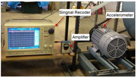
Figure 10.
Experimental setup for the rolling bearing fault diagnosis.
This study considered four bearing health conditions, including outer-race fault, inner-race fault, roller element fault and normal. Bearings under each health condition were operated at 800 rpm rotating speeds. These fault bearings are shown in Figure 11. In this experiment, the data set contained 2000 groups of training data, and each training sample contained 2400 sampling points. The standardized fault samples under each fault state were randomly divided into training data set and test data set with the scale of 7:3. We selected the same amount of data under each operating condition, 350 samples were used as the training set and 150 samples were used as the test set. In this way, this method ensured the balance of data and facilitated the diagnosis model to get correct diagnosis results.
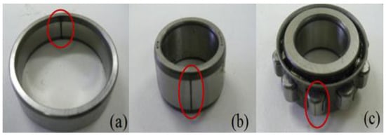
Figure 11.
Bearing fault: (a) outer-race fault, (b) inner-race fault, and (c) roller element fault.
4.3.2. Bearing Fault Diagnosis Experiment
Fault Diagnosis Results and Evaluation of the Proposed INPSO Optimization Method
During the optimization stage of SVM parameters (penalty factor c and the kernel parameter g), the proposed INPSO approach was adopted to tune appropriate parameters to improve fault diagnosis accuracy. The parameter settings of the algorithm were the same as in case 1. A group of samples was randomly selected as the test set, and the proposed 1DCNN was applied for feature extraction. Then the extracted feature vectors were respectively fed into the INPSO-SVM classifier, the SVM and PSO-SVM classifiers which were implemented as comparisons in this study. Each method was performed 10 times to reduce the effect of randomness and the diagnosis accuracy of the three classifiers are listed in Table 7. From Table 7, it can be seen that the fault diagnosis accuracy of SVM was only 91.98% without the parameters tuning process. In addition, the PSO-SVM performed better than SVM, where the average fault diagnosis accuracy was 93.3% with a standard deviation of 0.13. With the same test set, the proposed INPSO-SVM achieved the best performance in each trial and the average fault diagnosis could reach 94.186%. The standard deviation was 0.06, which indicated that the INPSO-SVM had good stability. Therefore, it could be concluded that the proposed algorithm had a stronger global optimization ability and played an important role in improving fault diagnosis accuracy.
Table 7.
The influence of parameter optimization on fault diagnosis accuracy.
Comparisons Among Different Fault Diagnosis Methods
In order to further prove that the proposed 1DCNN-INPSO-SVM could extract robust features and improve fault diagnosis accuracy, the WPT-INPSO-SVM method was used for comparative analysis. In the comparative experiments, the points to emphasize were the same as in case 1. The classification accuracies were evaluated and compared in Table 8. Table 8 lists the results obtained using the random 10 sets of data, where each set of data was used to test the 1DCNN-INPSO-SVM and the WPT-INPSO-SVM ten times respectively. The last column of Table 8 indicates that the proposed method achieved better performance, with the highest accuracy of 97.186%, while the competitor utilizing the features extracted by WPT obtained a lower accuracy.
Table 8.
Recognition results of ten trials using different methods.
5. Conclusions
As a promising machine learning algorithm, the convolutional neural network has been successfully applied in the field of intelligent fault diagnosis. In this paper, a novel hybrid fault diagnosis approach based on 1DCNN and INPSO-SVM is proposed for the fault diagnosis of rolling bearings. Firstly, the raw fault data is directly adopted as the inputs of the 1DCNN model to complete the training of CNN model, which can extract the invariant features of the original vibration signals. Moreover, in order to overcome the shortcomings of the basic PSO algorithm, e.g., trapping in the local optimums, a novel PSO variant INPSO is proposed, which combines two efficient strategies: Lévy flight and Chaos based initialization strategy. Finally, INPSO is used to tune the parameters of SVM and the features extracted by 1DCNN are used as the input of the INPSO-SVM classifier for fault classification. The proposed model can directly process the original vibration signals without any time-consuming manual feature extraction process. In addition, this method combines the excellent classification performance of SVM for small samples and the strong feature learning abilities of the CNN network, which avoids the problems of low representativeness and poor discrimination of traditional manual feature extraction, and improves the fault diagnosis accuracy. The INPSO algorithm is proposed to realize the automatic optimization of SVM parameters, which facilities the efficiency of SVM parameter optimization.
Extensive experiments were carried out to illustrate the effectiveness of the proposed method. First of all, numerical optimization experiments were conducted based on 8 widely applied benchmark functions and the simulation results indicated that the proposed PSO variant had a better performance in searching accuracy and convergence speed. Then, the feature learning ability of the 1DCNN was compared with three other feature extraction methods, including WPT, CAE and LSTM. The feature extraction results, which were presented in a novel visual manner, showed that the 1DCNN achieved a better performance. Finally, two cases of rolling bearing fault diagnosis experiments were carried out and experimental results showed that the proposed 1DCNN-INPSO-SVM hybrid framework was capable of diagnosing with high precision for rolling bearings and superior to some traditional fault diagnosis methods.
However, the proposed 1DCNN-INPSO-SVM does not use the temporal features of the vibration signals. The future work will focus on the extraction and utilization of the spatial-temporal characteristics. In addition, how to reduce the computational load and speed up the training process still deserve further study.
Author Contributions
Conceptualization, Y.S. (Yang Shao) and X.Y.; investigation, Y.S. (Yang Shao), X.Y. and Y.S. (Yang Song); methodology, Y.S. (Yang Shao) and X.Y.; software, Y.S. (Yang Shao); supervision, X.Y. and C.Z.; validation, Y.S. (Yang Shao), X.Y. and Q.X.; writing–original draft, Y.S. (Yang Shao) and X.Y. All authors have read and agreed to the published version of the manuscript.
Funding
This work is supported by the National Natural Science Foundation of China (Grant No. 61803227, 61973184, 61773242, 61603214), the National Key R & D Program of China (Grant No.2017YFB1302400), Independent Innovation Foundation of Shandong University (Grant No. 2082018ZQXM005).
Acknowledgments
We would like to thank the editors and the anonymous reviewers for their insightful comments and constructive suggestions.
Conflicts of Interest
The authors declare that there is no conflict of interests regarding the publication of this paper.
References
- Wang, S.; Selesnick, I.; Cai, J.; Feng, Y.; Sui, X.; Chen, X. Nonconvex sparse regularization and convex optimization for bearing fault diagnosis. IEEE Trans. Ind. Electron. 2018, 65, 7332–7342. [Google Scholar] [CrossRef]
- Jia, F.; Lei, Y.R.; Lu, N.; Xing, S. Deep normalized convolutional neural network for imbalanced fault classification of machinery and its understanding via visualization. Mech. Syst. Signal Process. 2018, 110, 349–367. [Google Scholar] [CrossRef]
- Jiang, W.; Cheng, C.; Zhou, B.; Ma, G.; Yuan, Y. A Novel GAN-based Fault Diagnosis Approach for Imbalanced Industrial Time Series. arXiv 2019, arXiv:1904.00575. [Google Scholar]
- Lei, Y.; Jia, F.; Zhou, X.; Lin, J. A deep learning-based method for machinery health monitoring with big data. J. Mech. Eng. 2015, 51, 49–56. [Google Scholar] [CrossRef]
- Sun, Y.; Gao, H.; Hong, X.; Song, H.; Liu, Q. Fault Diagnosis for Rolling Bearing Based on Deep Residual Neural Network. In Proceedings of the 2018 International Conference on Sensing, Diagnostics, Prognostics, and Control (SDPC), Xi’an, China, 15–17 August 2018. [Google Scholar]
- Zhao, M.; Kang, M.; Tang, B.; Pecht, M. Deep residual networks with dynamically weighted wavelet coefficients for fault diagnosis of planetary gearboxes. IEEE Trans. Ind. Electron. 2018, 65, 4290–4300. [Google Scholar] [CrossRef]
- Bi, F.; Ma, T.; Wang, X. Development of a novel knock characteristic detection method for gasoline engines based on wavelet-denoising and EMD decomposition. Mech. Syst. Signal. Process. 2019, 117, 517–536. [Google Scholar] [CrossRef]
- Tong, Z.; Li, W.H.; Zhang, B.; Li, B. Bearing fault diagnosis based on domain adaptation using transferable features under different working conditions. Shock. Vib. 2018, 2018, 1–12. [Google Scholar] [CrossRef]
- Chen, H.; Jiang, B.; Chen, W.; Yi, H. Data-Driven detection and diagnosis of incipient faults in electrical drives of high-speed trains. IEEE Trans. Ind. Electron. 2019, 66, 4716–4725. [Google Scholar] [CrossRef]
- Pan, L.; Zhu, D.; Shen, S.; Song, A.; Shi, X.; Duan, S. Gear fault diagnosis method based on wavelet-packet independent component analysis and support vector machine with kernel function fusion. Adv. Mech. Eng. 2018, 10, 1–10. [Google Scholar] [CrossRef]
- Tong, Z.; Li, W.; Zhang, B.; Jiang, F.; Zhou, G. Online bearing fault diagnosis based on a novel multiple data streams transmission Scheme. IEEE Access 2019, 7, 66644–66654. [Google Scholar] [CrossRef]
- He, Z.; Cheng, J.L.; Yang, Y. Linear maximum margin tensor classification based on flexible convex hulls for fault diagnosis of rolling bearings. Knowl. Based Syst. 2019, 173, 62–73. [Google Scholar] [CrossRef]
- Imani, M.; Dougherty, E.R.; Braga-Neto, U. Boolean Kalman filter and smoother under model uncertainty. Automatica 2020, 111, 108609. [Google Scholar] [CrossRef]
- Imani, M.; Ghoreishi, S.F. Bayesian Optimization Objective-Based Experimental Design; American Control Conference (ACC): Denver, CO, USA, 2020. [Google Scholar]
- Shao, H.; Jiang, H.; Lin, Y.; Li, X. A novel method for intelligent fault diagnosis of rolling bearings using ensemble deep auto-encoders. Mech. Syst. Signal. Process. 2018, 102, 278–297. [Google Scholar] [CrossRef]
- Gong, W.; Chen, H.; Zhang, Z.; Zhang, M.; Wang, R.; Guan, C.; Wang, Q. A novel deep learning method for intelligent fault diagnosis of rotating machinery based on improved CNN-SVM and multichannel data fusion. Sensors 2019, 19, 1693. [Google Scholar] [CrossRef]
- Chen, P.; Yuan, L.; He, Y. Deep learning. Neurocomputing 2015, 521, 436–444. [Google Scholar]
- Hinton, G.E.; Salakhutdunov, R.R. Reducing the dimensionality of data with neural networks. Science 2006, 313, 504–507. [Google Scholar] [CrossRef]
- Chen, P.; Yuan, L.; He, Y. Gearbox fault identification and classification with convolutional neural networks. Shock. Vib. 2016, 211, 202–211. [Google Scholar] [CrossRef]
- Wang, Q.; Zhao, B.; Ma, H.; Chang, J.; Mao, G. Fault diagnosis method based on FFT-RPCA-SVM for cascaded-multilevel inverter. ISA Trans. 2015, 2015, 1–10. [Google Scholar] [CrossRef]
- Janssens, O.; Slavkovikj, V.; Vervisch, B. Convolutional neural network based fault detection for rotating machinery. J. Sound Vib. 2016, 337, 331–345. [Google Scholar] [CrossRef]
- Fu, W.; Tan, J.; Zhang, X.; Chen, T.; Wang, K. Blind parameter identification of MAR model and mutation hybrid GWO-SCA optimized SVM for fault diagnosis of rotating machinery. Complexity 2019, 51, 1–17. [Google Scholar] [CrossRef]
- Yan, X.; Jia, M. A novel optimized SVM classification algorithm with multi-domain feature and its application to fault diagnosis of rolling bearing. Neurocomputing 2018, 313, 47–64. [Google Scholar] [CrossRef]
- Li, H.; He, C.; Malekian, R.; Li, Z. Weak defect identification for centrifugal compressor blade crack based on pressure sensors and genetic algorithm. Sensors 2018, 18, 1264. [Google Scholar] [CrossRef] [PubMed]
- Hao, X.; Zhang, G.; Ma, S. Deep Learning. Proc. Int. J. Semant. Comput. 2016, 10, 417–439. [Google Scholar] [CrossRef]
- Zhang, W.; Peng, G.; Li, C.; Chen, Y.; Zhang, Z. A new deep learning model for fault diagnosis with good anti-noise and domain adaptation ability on raw vibration signals. Sensors 2017, 17, 425. [Google Scholar] [CrossRef] [PubMed]
- Xia, M.; Li, T.; Xu, L.; Liu, L.; Silva, C. Fault diagnosis for rotating machinery using multiple sensors and convolutional neural networks. IEEE/ASME Trans. Mechatron. 2018, 23, 101–110. [Google Scholar] [CrossRef]
- Zheng, J.; Pan, H.; Cheng, J. Rolling bearing fault detection and diagnosis based on composite multiscale fuzzy entropy and ensemble support vector machines. Mech. Syst. Signal Process. 2017, 85, 746–759. [Google Scholar] [CrossRef]
- Vapnik, V.; Liu, L. The Nature of Statistical Learning Theory; Springer Science & Business Media: Berlin/Heidelberg, Germany, 2013. [Google Scholar]
- Teng, Z.; Lv, J.; Guo, L. An improved hybrid grey wolf optimization algorithm. Soft Comput. 2019, 23, 6617–6631. [Google Scholar] [CrossRef]
- Oliveira, J.; Oliveira, P.M.; Cunha, J.B.; Pinho, T. Chaos-based grey wolf optimizer for higher order sliding mode position control of a robotic manipulator. Nonlinear Dyn. 2017, 90, 1353–1362. [Google Scholar] [CrossRef]
- Yuan, X.; Jin, P.; Zhou, G. An improved QPSO algorithm integrating social learning with levy flights. Syst. Sci. Control. Eng. 2019, 6, 362–373. [Google Scholar]
- Zhang, W.; Peng, G.; Li, C.; Chen, Y. Antlion optimization algorithm integrating with Levy flight and golden sine. Appli. Res. Comput. 2018, 37, 1–6. [Google Scholar]
- Loparo, K. Case Western Reserve University Bearing Data Center, Cleveland, OH, USA, Tech. Rep. 2012. Available online: http://csegroups.case.edu/bearingdatacenter/pages/download-data-file (accessed on 28 September 2018).
- Zhang, W.; Li, C.; Peng, G.; Chen, Y.; Zhang, Z. A deep convolutional neural network with new training methods for bearing fault diagnosis under noisy environment and different working load. Mech. Syst. Signal Process. 2018, 100, 439–453. [Google Scholar] [CrossRef]
- Li, K. School of Mechanical Engineering, Jiangnan University. 2019. Available online: http://mad-net.org:8765/explore.html?t=0.5831516555847212 (accessed on 12 September 2019).


© 2020 by the authors. Licensee MDPI, Basel, Switzerland. This article is an open access article distributed under the terms and conditions of the Creative Commons Attribution (CC BY) license (http://creativecommons.org/licenses/by/4.0/).