Abstract
This paper presents a control method based the lateral interconnected air suspension system, in order to improve the road handling of vehicles. A seven-DOF (Degree of freedom) full-vehicle model has been developed, which considers the features of the interconnected air suspension system, for example, the modeling of the interconnected pipelines and valves by considering the throttling and hysteresis effects. On the basis of the well-developed model, a sliding mode controller has been designed, with a focus on constraining and minimizing the roll motion of the sprung mass caused by the road excitations or lateral acceleration of the vehicle. Moreover, reasonable road excitations have been generated for the simulation based on the coherence of right and left parts of the road. Afterwards, different simulations have been done by applying both bumpy and random road excitations with different levels of roughness and varying vehicle lateral accelerations. The simulation results indicate that the interconnected air suspension without control can improve the ride comfort, but worsen the road handling performance in many cases. However, by applying the proposed sliding mode controller, the road handling of the sprung mass can be improved by 20% to 85% compared with the interconnected or non-interconnected mode at a little cost of comfort.
1. Introduction
The vehicle suspension plays an important role in reducing the body vibration transmitted from the road excitations and ensuring handling stability of vehicles [1,2]. With the increasing demand on ride comfort and road handling, various control technologies and structures of suspensions are emerging continuously.
Vehicle suspensions can be classified into three types: active [3,4,5,6], semi-active [7,8,9,10,11,12], and passive [13,14,15,16]. Active suspension systems with appropriate control strategies can greatly improve both the comfort and handling, but they are expensive and consume large amounts of energy. Thus, energy-regenerative structures are proposed to reduce power consumption, resulting in more complex structure and costs [17,18,19,20]. Passive suspension systems with constant spring stiffnesses and damping coefficients only perform well under limited conditions, but new structures have also recently been proposed to improve the overall performance [20,21]. Meanwhile, semi-active suspension systems can reach a balance between cost and performance, thus the research of semi-active suspensions attracts lots of attention.
In terms of the semi-active suspension, the air spring has been widely used because of its significant advantages of low vibration-transfer coefficient and adaptive load-capacity ability [22,23,24]. In addition, the air spring is applicable for adjusting the body height or tuning the stiffness, which brings more control flexibility to the semi-active suspension [25,26,27,28]. Some new structures of the air spring have been proposed, such as the air suspension with an additional air chamber and the interconnected air suspension [29,30,31]. Generally, connecting the air spring to an additional chamber can soften the air spring. Similarly, the interconnected air suspension system connects springs with a pipeline, and each connected spring plays the role of the others’ additional chamber. However, different from the additional-chamber design, the sum gas volume of all the springs remains constant in the interconnected suspension system. Therefore, the vertical stiffness of the vehicle stays the same and only the roll and pitch dynamics are affected [31,32]. Besides, the pitch and roll dynamics affect the bounce response of the vehicle body [33,34,35], which brings the opportunity to improve the suspension performance via interconnection.
Interconnected suspension can be classified based on the transferred media, for example, mechanical, hydraulically, pneumatic, and hydro-pneumatic interconnected suspension [31,36,37,38,39]. The interconnected air suspension was proposed by Higginbotham in BHL in 1961 [40], which can be interconnected laterally and longitudinally. The longitudinally interconnected air suspension is mainly used in heavy trucks to achieve better road friendliness and ride comfort [41,42]. Hence, many studies can be found in the literature, such as modeling, characteristics analysis, structural optimization, and the corresponding control strategies [28,42,43]. Similarly, the laterally interconnected systems can also improve the road friendliness and comfort. On the basis of previous studies [22,31], the effect of the interconnection mostly depends on the diameter and length of the interconnection pipelines. The lateral interconnection structure significantly reduces the pipeline length compared with the longitudinal one. Thus, the laterally interconnected suspension system has a quicker response and achieves better comfort and road friendliness than the longitudinal one when using the same diameter of the pipelines.
However, the current studies on laterally interconnected air suspension system only focus on its modeling and characteristic analysis. To achieve a better use of laterally interconnected suspension system, an appropriate control method should be developed. Several methods have been proposed to overcome different shortcomings. Cui presented a simple condition-based control method according to the characteristics of the interconnected air suspension. Technically, it involves turning on or off the interconnection according to the vehicle speed, steering angle, and the roll angle of the sprung mass [44]. This method achieves a balance between handling and comfort. However, the coherence of the right and left parts of the road has not been considered, and owing to the rough classifications of the conditions, the proposed control method is not efficient and convincing enough. Moreover, Ju proposed an imitated skyhook control strategy, which gets rid of the estimation of vehicle speed and steering angle. Furthermore, it can adjust the performance weights between handling and comfort by changing its control parameters [45]. Essentially, however, it is just a trade-off between interconnection and non-interconnection.
In order to improve the handling and the safety, a sliding mode control method is proposed. The nonlinear characteristics of the interconnection pipelines and air springs are taken into consideration [29,41,42]. Because the performance of the laterally interconnected air suspension is strongly affected by the excitations of the right and left wheels, the coherence of left and right part of the roads is taken into consideration to present more fair and real results. Furthermore, different from other control strategies that aim to provide a balance between comfort and handling, the proposed control method focuses on improving the handling and safety of the laterally interconnected air suspension, and achieves a better roll motion than both the interconnected and non-interconnected suspensions under all scenarios.
This paper is organized as follows. Firstly, a nonlinear vehicle model equipped with the air suspensions system is introduced, and then the interconnection pipelines are modeled by considering the throttling and hysteresis effects. Secondly, to illustrate the effectiveness of the control strategy fairly, road excitations are generated based on the coherence of right and left parts of the road. Thirdly, the sliding mode controller is designed based on the constant rate reaching law. Finally, varying simulations are conducted to evaluate the performance of the sliding mode controller and compare with the imitated skyhook controller. In addition, the performance of interconnected air suspensions and non-interconnected air suspensions are also discussed.
2. Full Vehicle Modeling and Road Excitations
This section describes the modeling process of a full vehicle model with interconnected air suspensions and the generation of random road excitations.
2.1. Modeling of the Vehicle and Air Suspensions
Considering that the deformation speed of each air spring is no more than 15 m/s, while the air pressure transfers at a speed of 345 m/s, we assume that the thermodynamic state within each air spring is equal. Meanwhile, during work time, the air pressure of each spring is no more than 1 MPa and the temperature is much higher than 0 K, thus the air can be treated as ideal gas with acceptable error. In addition, the air spring has less heat exchange with outside world, which can be treated as an adiabatic process.
On the basis of the assumptions above and thermodynamic theory, air states in air spring can be described as
where I = 1,2,3,4 represents each air spring in this paper; Pi is the pressure of each air spring; Vi is the volume of each air spring; mi is the air mass of each air spring; κ is adiabatic exponent and equals to 1.4; and const means a constant.
Assuming no mass flow leakage in the system components, the pressure of each air spring at any time can be calculated with Equation (2)
where Pi0, Vi0, and mi0 represent the initial pressure, volume, and air mass of each air spring, respectively. The parameters Vi and mi can be expressed as
where dVi/dh is the volume change rate with height of each air spring. fdi is the suspension travel of each suspension. qai represents the air mass flow in and out of each air spring, which can be calculated with the interconnection model in the next section.
Moreover, the effect area of the air spring also varies with the suspension travel, thus the effect area Aei of each air spring can be calculated as
where Aei0 is the initial effect area of each air spring and dAei/dh is the effect area change rate with height of each spring.
Hence, the force of air spring can be expressed as
where Pa is the atmospheric pressure and equals to 1 × 10⁵ Pa.
For control purposes, this study utilizes a simplified seven-DOF suspension model. The more realistic vehicle suspension model and damper model can be found in [46,47]. The full-vehicle dynamic model with air suspension feature is established for modeling the entire system, which comprises the vertical, roll, and pitch movements of the body and vertical movements of four wheels, as shown in Figure 1.
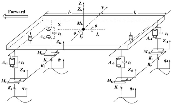
Figure 1.
A seven-DOF full-vehicle dynamic model for vertical vibration.
On the basis of Newton’s law and vehicle dynamics, the seven-DOF full vehicle model can be formulated as follows
where
where Mb is the sprung mass; Zb is the vertical displacement of the body centroid; Ir and θ are the rotational inertia of the body around the X-axis and the body roll angle, respectively; Ip and φ are the rotational inertia of the body around Y axis and the body pitch angle, respectively; lf and lr are the distances from front and rear axles to the body centroid, respectively; Bf and Br are the distances between front and rear wheel tread, respectively; ci is the damping of each suspension; Mti is the unsprung mass of the ith corner of the vehicle; Zti is the vertical displacements of each unsprung mass; Kt is the vertical stiffness of each tire; qi is the the vertical displacement excitations of four wheels, respectively; and fdi is the suspension travel of each suspension. The interconnection pipelines and valves are also illustrated in the figure; the valves are located in the middle of the pipelines.
2.2. Model of Interconnection Pipeline and Valve
As mentioned in Equation (4) above, the air mass in each spring changes as the air flows in and out of the spring. When the interconnection state is “ON” and the pressures of two air springs are different, the air will flow from the high-pressure side to the low-pressure side and changes the pressure of the two air springs, leading to a varying of spring forces.
During the progress of air exchanging, two main effects will be involved with the air passing through the interconnection pipeline and valve: one is the throttling effect and the other is the hysteresis effect. The transients of the valve are ignored in this paper as the response delay of the high-speed valve is much smaller than the hysteresis effect of the pipelines. Thus, the interconnection part can be treated as a combination of a throttle hole and a pipeline with the hysteretic effect.
Considering a throttle hole model and ignoring the dynamic property, the static area-normalized mass flow through the hole can be expressed as [48]
where qa is the air mass flow in the pipeline; Se is the flow coefficient and equals 0.7 in this model; S is the effect area of the hole; Pu and Pd are the upstream and downstream pressure, respectively; Tu is the upstream air temperature of the spring; R is perfect gas constant, and as with the air, equals 287 N∙m/(kg∙K); and Pu/Pd is pressure ratio and the comparison of the pressure ratio and the critical pressure ratio decides the flow type.
After the air mass comes through the throttle, it still needs to travel along the pipeline. At this progress, the friction occurs between the air flow and the inner wall of the pipeline, which results in the loss of energy and leads to the pressure of the air drops along the direction of its flow. Meanwhile, owing to the speed of the flow, a delay will be involved in the response of air mass between the outlet and inlet end of the pipeline. Considering those effects above, the function of the air mass flow in the different position of the pipeline changing with time can be described as
where L is the length of the pipeline; Vd and md are the downstream volume and air mass of the spring, respectively; vc is the sound velocity and equals 345.2 m/s at 25 ℃; and Rt is the resistance coefficient of the inner wall of the pipeline. As the air flow is mostly laminar flow when the interconnected air suspension works, Rt can be calculated as follows
where μ is air flow viscous coefficient and equals 1.8 × 10⁻⁵ Pa∙s at 25 ℃ and D is the diameter of the pipeline.
Associated with Equations (2)–(6) above, when the air springs are laterally interconnected, the forces of each air spring can be calculated, and hence the seven-DOF full vehicle model of laterally interconnected air suspension is established.
2.3. Generation of Road Excitations
In order to accurately describe the performance of laterally interconnected air suspensions, a reasonable road excitation model should be built.
According to [49,50,51], the road roughness input in the time domain can be expressed by
where q(t) represents the road vertical displacement in time domain. fmid-i is the ith middle frequency of ith part. Gq(fmin-i) is PSD (Power spectral density) of fmid-i. Φi is the independent and identically distributed (IID) random phase within (0.2 π). fa and fb are lower and upper frequency bounds, respectively. Considering that the commonly used vehicle speed v ranges from 10~30 m/s, and the lower and upper spatial frequency are set to 0.011/m and 2.83/m according to ISO 8608, the fa and fb should be equal to 0.33 Hz and 28.3 Hz, respectively.
Road profiles of left and right wheels are different, but not independent. Dieter Ammon presents a widely used method for calculating the coherence γ(Ω,Tw) of left and right side of the road profiles, as [52,53,54]
where Ω is the angular spatial frequency of the road, Tw is the track width, W is the frequency exponent and equals 2, p is the reference coefficient, Ωp is the reference angular spatial frequency, and a is a constant exponent of Tw. For the isotropic process, a = 1.
Considering two given road vertical displacements q1(t) and q2(t) for left and right side of wheels, the transfer function G(s) of q1(t) and q2(t) can be written as
where Q1(s) and Q2(s) are the Laplace transform of q1(t) and q2(t), respectively. Taking the coherence γ(Ω,Tw) in Equation (13) into consideration, the norm of this transfer function should be equal to the norm of γ(Ω,Tw). Thus, a Pade algorithm is applied and a GA (genetic algorithm) method is used to obtain acceptable parameters of this transfer function [46]. The result of the transfer functions is marked as G12(s) in this paper.
Assuming that the vehicle runs along under a straight-line condition, the road profiles for rear wheels are roughly the same as those of front wheels, except a time delay is involved. Therefore, the left and right road vertical displacements q3(t) and q4(t) for rear axle can be expressed as follows
where t ≥ τ and τ are the delay time lying on the track width and vehicle speed, respectively, and τ = (lf + lr)/v in this paper.
Recall the road vertical displacement for one wheel in time domain can be calculated with Equation (12); firstly, two road vertical displacements q1 0(t) and q2 0(t) in the time domain are generated separately, then the road excitations for four wheels can be generated with q1 0(t), q2 0(t), and the coherence transfer function above, as Figure 2a shows the generated random C-class road excitations at a 20 m/s vehicle speed. The PSD of roads for the front left and front right wheels are illustrated in log-log scale in Figure 2b, which also contains the roughness indexes information classified by ISO. Those two figures illustrate the model the road excitations are current enough to use.
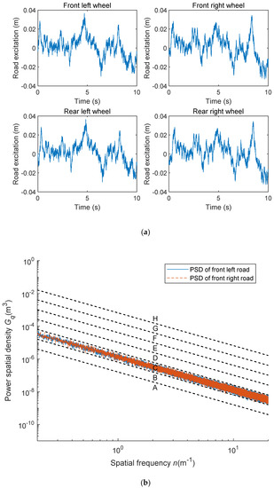
Figure 2.
The generated road excitations: (a) C-class road profile for four wheels; (b) road roughness classification and PSD of generated front left and right road.
3. Sliding Mode Controller for Interconnection
The main aim of the controller is to minimize the roll angle subject to road disturbances, thereby providing better handling.
Considering that the interconnection decouples the vertical and roll vibrations and only has an effect on the roll movement of the sprung mass, let e be the error, defined as
where θref is the reference roll angle of sprung mass and equals 0.
Let C = [c,1], error vector E = , then the sliding surface s is defined as follows
By selecting the Lyapunov function,
To ensure the existence and attractiveness of the sliding mode surface, it is sufficient to choose a control law such that
Therefore, the sliding mode controller is designed by the constant rate reaching law to meet the above condition:
where δ > 0 is the sliding mode switching control gain. When the generalized sliding mode arrival condition , the approaching law will be satisfied. Combining the nonlinear and coupling characteristics of the interconnected air suspension, the control law can be calculated step by step.
According to Equation (17) and (18), and considering that θref is a constant and equals 0, Equation (21) can be expressed as
Noticing that can be replaced according to Equation (7)
Because the torques for the sprung mass roll motion provided by suspensions of front and rear axles are related to the pressure of each air spring, F1-F2 and F3-F4 can be calculated as follows
According to Equation (8), each suspension force includes spring force and damping force, and the spring force can be calculated with the effect area Aei, volume Vi, and air mass mi, and the initial pressure pi0 of the air spring depends on Equation (2). Among them, only air mass has matters with the interconnection control. Thus, Equation (24) can be written as
where
where Aei and Vi can be calculated with Equations (5) and (3).
Considering that the interconnection only makes the air mass flow from one air spring to the other, the total air mass among the air springs is a constant, thus an optimization problem can be established to find the expected air mass mi of each air spring that best meet Equation (25) within the range of [0, m(2j−1)0+m(2j)0], j = 1,2. Minimizing the square values of the left and right sides’ differences of Equation 25 as the optimization target, the problem can be described as follows
The optimization problem can be easily solved with a certain numerical error tolerance, and the air mass of each air spring can be obtained as mir. According to Equation (4), the air mass flow in and out of each air spring can be the differential of mir, that is, .
The air flows from the high-pressure area to the low-pressure area, hence assuming that the direction of air mass flows into the left side air spring is positive, that is to say,
where j = 1, 2. qasi means the value of air mass flows into the front left, front right, rear left, and rear right air springs, respectively. S1 and S2 are the interconnection pipeline effect areas of front and rear axles.
According to Equation (28) above and the results of Equation (27), the effect areas of interconnection pipelines can be calculated as
where Sjr (j = 1, 2) are the effect areas of each interconnection pipelines.
The calculation is divided into five parts according to the directions of air mass flow m1r, m3r and the pressure differences of P1, P2 and P3, P4. When the directions of air mass flow have different signs from the pressure differences, the interconnections are shut, that is, the effect areas of the interconnection pipelines are set to 0. When the directions of air mass flow have the same signs as the pressure differences, the effect areas of each interconnection pipelines calculated with the pressures and temperatures of each air springs and the flow types accordingly.
Owing to the space restriction, the interconnection pipeline has a limited diameter. The maximum diameter of the pipeline is 0.02 m in this paper. Thus, the maximum effect area is 3.142 × 10⁻⁴ m2, and the control vector u is as follows
4. Simulations and Analysis
To validate the effectiveness of the proposed controller, simulations of different controllers are conducted in MATLAB/Simulink environment. In this section, the time responses of sprung mass roll angle and the acceleration of front left sprung mass corner are performed under contrary road input and lateral acceleration input, and the root square mean (RMS) values of roll angle and acceleration of front left sprung mass corner are also calculated under different road roughness levels and vehicle speeds.
4.1. Simulation Settings
On the basis of the nonlinear full car interconnected air suspension model established above, two types of controllers are applied to make a comparison, which are approached sliding mode controller and imitated skyhook controller, and the “ON” and “OFF” interconnection states are also taken into consideration in the simulation. The skyhook controller for interconnection is a kind of control strategy that imitates the Skyhook damper controller, when the roll angle of sprung mass has a different sign from the sprung mass roll angle minus the axle roll angle, the interconnection remains “ON”; when the sprung mass roll angle has the same sign as sprung mass roll angle minus the axle roll angle, the interconnection remains “OFF” [44].
Table 1 shows all the parameters used in this full-vehicle model, which are measured based on a commercial vehicle and have been verified by test in previous work [44].

Table 1.
Simulation parameters for full car model.
4.2. Simulation Results Under Varying Situations
As the roll movement is mainly caused by the unequal excitation of left and right side of the road, a right-left twisted road input is firstly applied. The left side of the road raises 5 mm at 0 s, while the right side of the road drops 5 mm at the same time.
Figure 3a shows the roll angle responses of sprung mass with different interconnection states or controllers under the applied excitations. Here, the “ON” state means that the suspension is interconnected air suspension, while the “OFF” state means that the suspension is non-interconnected air suspension. The “imitated skyhook” and “sliding mode” represent that using the imitated skyhook controller or the sliding mode controller to control the on and off states of the interconnection.
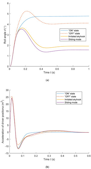
Figure 3.
The response of the vehicle under banked road excitations: (a) roll angles of sprung mass; (b) accelerations of driver position.
When laterally connected, the steady-state value of the roll angle is higher than others under the applied road input condition, but the peak value of the roll angle drops compared with the “OFF” state. The imitated skyhook controller can reduce the roll angle obviously, but the sliding mode controller performs the best in reducing the steady-state and peak value of the response. Under the applied road excitations, the sliding mode controller reduces the roll angle by 72% compared with the “ON” state and 41% peak value of roll angle response compared with the “OFF” state.
Figure 3b shows the acceleration responses of driver position. It illustrates that, with the “OFF” state of the interconnection, the acceleration response will reach higher peak and valley values under the applied excitation. Moreover, keeping the interconnection in the “ON” state will result in the acceleration response coming to the balance position much faster than other methods. The imitated skyhook controller and the sliding mode controller lead to approximately the same acceleration responses. Both increase by 4.9% in RMS of the responses compared with the “ON” state and 4.6% in amplitude compared with the “OFF” state.
In Equation (31), the lateral acceleration is added considering the same road excitations of the vehicle runs along under a straight line.
where ay is the lateral acceleration, and Hr is the distance from the centroid to roll axis and equals 0.3 m.
An excitation of 3 m/s2 lateral acceleration is applied at 0 second in the simulation; Figure 4a,b show the performance with each method.
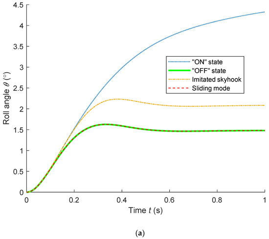
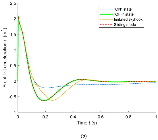
Figure 4.
The response of the vehicle under lateral acceleration: (a) roll angles of sprung mass; (b) accelerations of driver position.
The above figures show that, under the lateral acceleration excitation, the imitated skyhook controller makes a balance between the acceleration and roll angle, it reduces the amplitude of acceleration response compared with “ON” state, while increasing the steady-state value of roll angle response compared with the “OFF” state. Meanwhile, the sliding mode controller chooses to shut the interconnection. This action is reasonable as it is aimed at minimizing the roll angle and the performance is the same as the “OFF” state. Thus, under the applied excitation, the sliding mode controller manages to drop 63% of the steady-state value of roll angle response compared with the “ON” state, while it raises 58% and 86% of the peak and RMS values of the acceleration response.
Furthermore, simulations are conducted under varying road roughness levels and lateral accelerations to evaluate the performance of sliding mode controller on actual driving conditions. Road excitations are established with roughness levels varying from A to E. The lateral accelerations are also added, which vary from 0 m/s2 to 3 m/s2 and step 0.2 m/s. Under each condition, the responses of roll angle and acceleration of driver position are recorded. Then, the RMS values of those records are calculated. Finally, the RMS values of all the roll angle records are presented in ratios using the “ON” state performance as a baseline. Meanwhile, the RMS values of all the acceleration records are presented in ratios using the “OFF” state performance as a standard.
Figure 5a,b show the results of the simulations.
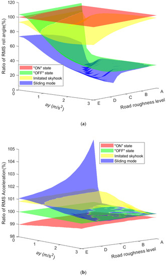
Figure 5.
The response of the vehicle under varying conditions: (a) ratio of root mean square (RMS) roll angle compared with the “ON” state; (b) ratio of RMS acceleration at driver position compared with the “OFF” state.
Figure 5a,b show that the interconnected air suspension performs better in reducing both roll angle and acceleration under straight driving condition no matter the road roughness levels, while the non-interconnected air suspension can reduce the roll angle notably when the lateral acceleration increases. The skyhook controller drops the roll angle under minor lateral acceleration excitations, but it is defeated by the “OFF” state when lateral acceleration increases. The RMS of roll angle responses remains the lowest under any conditions with the sliding mode controller, which declines 20% at least and 85% at most compared with the “ON” state.
In Figure 5a, the curve shows that the sliding mode controller is always better at reducing the roll angle compared with the “OFF” state, but in Figure 4a, the roll angles are the same. This is because the road excitations are added in the simulations of Figure 5a. When the road excitations change the sign of the pressures’ difference of two connected air springs, the sliding mode controller manages to turn on the interconnection, which changes the distributions of air mass in each spring and finally results in smaller RMS values. This phenomenon is illustrated in Figure 6 below. The vehicle drives in a straight line at time 0–10 and 60–70 seconds and in steady turning during 10–60 seconds. During this period, the sliding mode controller keeps the interconnection shut for most of the time, but turns the interconnection on several times and, each time, reduces the roll angle. Finally, the roll angle response of sliding mode controller reduces at a visible level compared with the “OFF” state.

Figure 6.
Gas exchange under cornering condition.
Because of the aim of reducing the roll angle, the performance of sliding mode controller is limited at acceleration decreasing. Figure 5b shows that the sliding mode controller increases the driver position acceleration by 5% for the A level road and 0 m/s2 lateral acceleration condition compared with the “OFF” state. However, the RMS values drops with the increase of road roughness levels and the lateral acceleration amplitudes. Finally, the RMS values are approximately the same with the “OFF” state. The skyhook controller performs better than the sliding mode controller when the lateral acceleration is small, but it fails when the lateral acceleration input grows. The “ON” state keeps the RMS values about 2% smaller compared with the “OFF” state under any situation, which agrees with the results in Figure 3b and Figure 4b.
In summary, the sliding mode controller gains great achievement in roll angle control at a cost of minor comfort lost. The skyhook controller performs better under small cornering maneuvers. The interconnected air suspension can improve both the handling and comfort under any road roughness levels when the lateral acceleration input is small.
5. Conclusions
This paper designed a controller for the lateral interconnection air suspension aiming at improving the handling performance. A nonlinear seven-DOF full-vehicle mode with interconnected air suspension feature was firstly built, where the throttling and hysteresis effect of the interconnection pipelines were considered. The road input was also well considered with the coherence of each side of the road.
As the lateral interconnection only affects the roll movement, as previous works mentioned, a sliding mode controller was established to reduce the roll angle by changing the interconnection of the air springs. The control law was calculated step by step according to the above nonlinear mode and the assumption that the roll torques provided by suspensions of front and rear axles have the same ratio with each axle loads.
The simulation results showed that, under right–left twisted road conditions, the sliding mode controller dropped around 70% steady-state value of roll angle at a cost of raising the peak and RMS values of acceleration. When under step lateral acceleration excitation, the sliding mode controller kept the interconnection off and performed the same as the non-interconnected suspension. Moreover, the sliding mode controller was most effective at improving the handling among all the situations, as a reduction of 20%~85% in RMS values of the roll angle only sacrifices a bit of comfort compared with the “ON” state. In summary, the sliding mode controller provides a solution in roll angle control of the interconnection air suspension, especially under varying working conditions.
Author Contributions
Software, D.G.; validation, T.S.; methodology, A.K.; writing—original draft preparation, Y.W.; writing—review and editing, T.S.; project administration, L.Z.; funding acquisition, L.Z. All authors have read and agreed to the published version of the manuscript.
Funding
This research was funded by National Natural Science Foundation of China, grant number No.51575241 and No.51305111, and the program of China Scholarship Council, grant number No.201808320255. The APC was funded by National Natural Science Foundation of China (No.51575241).
Acknowledgments
The authors would like to thank the National Natural Science Foundation of China and the program of China Scholarship Council for funding this research, and the support of Dr. Yanjun Huang.
Conflicts of Interest
The authors declare no conflict of interest.
References
- Marzbanrad, J.; Keshavarzi, A. Chaotic Vibrations of a Nonlinear Air Suspension System under Consecutive Half Sine Speed Bump. Indian J. Sci. Technol. 2015, 8, 72. [Google Scholar] [CrossRef]
- Tseng, H.E.; Hrovat, D. State of the art survey: Active and semi-active suspension control. Veh. Syst. Dyn. 2015, 53, 1034–1062. [Google Scholar] [CrossRef]
- Rath, J.J.; Defoort, M.; Karimi, H.R.; Veluvolu, K.C. Output Feedback Active Suspension Control With Higher Order Terminal Sliding Mode. IEEE Trans. Ind. Electron. 2017, 64, 1392–1403. [Google Scholar] [CrossRef]
- Huang, Y.; Na, J.; Wu, X.; Liu, X.; Guo, Y. Adaptive control of nonlinear uncertain active suspension systems with prescribed performance. ISA Trans. 2015, 54, 145–155. [Google Scholar] [CrossRef] [PubMed]
- Wen, S.; Chen, M.Z.Q.; Zeng, Z.; Yu, X.; Huang, T. Fuzzy Control for Uncertain Vehicle Active Suspension Systems via Dynamic Sliding-Mode Approach. IEEE Trans. Syst. Man, Cybern. Syst. 2016, 47, 24–32. [Google Scholar] [CrossRef]
- Zhang, H.; Zheng, X.; Yan, H.; Peng, C.; Wang, Z.; Chen, Q. Codesign of Event-Triggered and Distributed Filtering for Active Semi-Vehicle Suspension Systems. IEEE/ASME Trans. Mechatron. 2017, 22, 1047–1058. [Google Scholar] [CrossRef]
- Qin, Y.; Zhao, F.; Wang, Z.; Gu, L.; Dong, M. Comprehensive Analysis for Influence of Controllable Damper Time Delay on Semi-Active Suspension Control Strategies. J. Vib. Acoust. 2017, 139, 031006. [Google Scholar] [CrossRef]
- El Majdoub, K.; Ghani, D.; Giri, F.; Chaoui, F.Z. Adaptive Semi-Active Suspension of Quarter-Vehicle with Magnetorheological Damper. J. Dyn. Syst. Meas. Control. 2014, 137, 021010. [Google Scholar] [CrossRef]
- Sharma, S.K.; Kumar, A. Ride performance of a high speed rail vehicle using controlled semi active suspension system. Smart Mater. Struct. 2017, 26, 055026. [Google Scholar] [CrossRef]
- Nie, S.; Zhuang, Y.; Liu, W.; Chen, F. A semi-active suspension control algorithm for vehicle comprehensive vertical dynamics performance. Veh. Syst. Dyn. 2017, 96, 1–24. [Google Scholar] [CrossRef]
- Martini, A.; Bellani, G.; Fragassa, C. Numerical Assessment of a New Hydro-Pneumatic Suspension System for Motorcycles. Int. J. Automot. Mech. Eng. 2018, 15, 5308–5325. [Google Scholar] [CrossRef]
- Palomares, E.; Morales, A.L.; Nieto, A.J.; Chicharro, J.M.; Pintado, P. Modelling Magnetorheological Dampers in Preyield and Postyield Regions. Shock. Vib. 2019, 2019, 1–23. [Google Scholar] [CrossRef]
- Gadhvi, B.; Savsani, V.; Patel, V.K. Multi-Objective Optimization of Vehicle Passive Suspension System Using NSGA-II, SPEA2 and PESA-II. Procedia Technol. 2016, 23, 361–368. [Google Scholar] [CrossRef]
- Seifi, A.; Hassannejad, R.; A Hamed, M. Optimum design for passive suspension system of a vehicle to prevent rollover and improve ride comfort under random road excitations. Proc. Inst. Mech. Eng. Part K J. Multi-body Dyn. 2016, 230, 426–441. [Google Scholar] [CrossRef]
- Mitra, A.C.; Desai, G.J.; Patwardhan, S.R.; Shirke, P.H.; Kurne, W.M.; Banerjee, N. Optimization of Passive Vehicle Suspension System by Genetic Algorithm. Procedia Eng. 2016, 144, 1158–1166. [Google Scholar] [CrossRef]
- Odabaşı, V.; Maglio, S.; Martini, A.; Sorrentino, S. Static stress analysis of suspension systems for a solar-powered car. FME Trans. 2019, 47, 70–75. [Google Scholar] [CrossRef]
- Suda, Y.; Nakadai, S.; Nakano, K. Hybrid Suspension System with Skyhook Control and Energy Regeneration (Development of Self-Powered Active Suspension). Veh. Syst. Dyn. 1998, 29, 619–634. [Google Scholar] [CrossRef]
- Xie, X.; Wang, Q. Energy harvesting from a vehicle suspension system. Energy 2015, 86, 385–392. [Google Scholar] [CrossRef]
- Khoshnoud, F.; Zhang, Y.; Shimura, R.; Shahba, A.; Jin, G.; Pissanidis, G.; Chen, Y.K.; De Silva, C.W. Energy Regeneration From Suspension Dynamic Modes and Self-Powered Actuation. IEEE/ASME Trans. Mechatronics 2015, 20, 2513–2524. [Google Scholar] [CrossRef]
- Xu, X.; Sardahi, Y.; Zheng, C. Multi-Objective Optimal Design of Passive Suspension System With Inerter Damper. In Proceedings of the ASME 2018 Dynamic Systems and Control Conference, Atlanta, GA, USA, 30 September–3 October 2018; ASME: New York, NY, USA; p. V003T40A006, Paper No. DSCC2018-9011. [Google Scholar]
- Shen, Y.; Chen, L.; Yang, X.; Shi, D.; Yang, J. Improved design of dynamic vibration absorber by using the inerter and its application in vehicle suspension. J. Sound Vib. 2016, 361, 148–158. [Google Scholar] [CrossRef]
- Moheyeldein, M.; Abd-El-Tawwab, A.M.; El-Gwwad, K.A.; Salem, M. An analytical study of the performance indices of air spring suspensions over the passive suspension. Beni-Suef Univ. J. Basic Appl. Sci. 2018, 7, 525–534. [Google Scholar] [CrossRef]
- Zhu, H.; Yang, J.; Zhang, N.; Feng, X. A novel air spring dynamic model with pneumatic thermodynamics, effective friction and viscoelastic damping. J. Sound Vib. 2017, 408, 87–104. [Google Scholar] [CrossRef]
- Le, V.Q. Comparing the performance of suspension system of semi-trailer truck with two air suspension systems. Vibroeng. Procedia 2017, 14, 220–226. [Google Scholar] [CrossRef]
- Sun, X.; Cai, Y.; Wang, S.; Liu, Y.; Chen, L. A hybrid approach to modeling and control of vehicle height for electronically controlled air suspension. Chin. J. Mech. Eng. 2015, 29, 152–162. [Google Scholar] [CrossRef]
- Zhao, J.; Wong, P.K.; Xie, Z.; Wei, C.; He, F. Integrated variable speed-fuzzy PWM control for ride height adjustment of active air suspension systems. In Proceedings of the 2015 American Control Conference (ACC), Chicago, IL, USA, 1–3 July 2015; pp. 5700–5705. [Google Scholar]
- Zepeng, G.; Jinrui, N.; Lian, L.; Xiaolin, X. Research on Air Suspension Control System Based on Fuzzy Control. Energy Procedia 2017, 105, 2653–2659. [Google Scholar] [CrossRef]
- Eskandary, P.K.; Khajepour, A.; Wong, A.; Ansari, M. Analysis and optimization of air suspension system with independent height and stiffness tuning. Int. J. Automot. Technol. 2016, 17, 807–816. [Google Scholar] [CrossRef]
- Zhu, H.; Yang, J.; Zhang, Y. Modeling and optimization for pneumatically pitch-interconnected suspensions of a vehicle. J. Sound Vib. 2018, 432, 290–309. [Google Scholar] [CrossRef]
- Li, W.; Chen, Y.; Zhang, S.; Mao, E.; Du, Y.; Wen, H. Damping Characteristic Analysis and Experiment of Air Suspension with Auxiliary Chamber. IFAC-PapersOnLine 2018, 51, 166–172. [Google Scholar] [CrossRef]
- Jiang, H.; Wang, Z.; Kong, L. Neural-Fuzzy Control Applied in Adjustable Volume Air Suspension with Additional Air Chambers. J. Chongqing Univ. Technol. Nat. Sci. 2017, 3, 1. [Google Scholar]
- Xu, X.; Nannan, Z. Dynamic Modeling and Simulation Analysis of Interconnected Air Suspension System. SAE Tech. Paper Series 2016, 1. [Google Scholar] [CrossRef]
- Azman, M.; King, P.D.; Rahnejat, H. Combined bounce, pitch, and roll dynamics of vehicles negotiating single speed bump events. Proc. Inst. Mech. Eng. Part K J. Multi-body Dyn. 2007, 221, 33–40. [Google Scholar] [CrossRef]
- Azman, M.; Rahnejat, H.; King, P.D.; Gordon, T.J. Influence of anti-dive and anti-squat geometry in combined vehicle bounce and pitch dynamics. Proc. Inst. Mech. Eng. Part K J. Multi-Body Dyn. 2004, 218, 231–242. [Google Scholar] [CrossRef]
- Smith, M.C.; Walker, G.W. Interconnected vehicle suspension. Proc. Inst. Mech. Eng. Part D J. Automob. Eng. 2005, 219, 295–307. [Google Scholar] [CrossRef]
- Zou, J.; Guo, X.; Abdelkareem, M.A.; Xu, L.; Zhang, J. Modelling and ride analysis of a hydraulic interconnected suspension based on the hydraulic energy regenerative shock absorbers. Mech. Syst. Signal Process. 2019, 127, 345–369. [Google Scholar] [CrossRef]
- Ding, F.; Han, X.; Zhang, N.; Luo, Z. Characteristic analysis of pitch-resistant hydraulically interconnected suspensions for two-axle vehicles. J. Vib. Control. 2014, 21, 3167–3188. [Google Scholar] [CrossRef]
- Chen, Y.; Peterson, A.W.; Ahmadian, M. Achieving anti-roll bar effect through air management in commercial vehicle pneumatic suspensions. Veh. Syst. Dyn. 2018, 57, 1775–1794. [Google Scholar] [CrossRef]
- Chen, Y.; Ahmadian, M.; Peterson, A. Pneumatically Balanced Heavy Truck Air Suspensions for Improved Roll Stability. SAE Technical Paper Series 2015, 1. [Google Scholar] [CrossRef]
- Higginbotham, W. Interconnected Air Suspension. U.S. Patent 2,988,372, 13 June 1961. [Google Scholar]
- Chen, Y.; He, J.; King, M.; Chen, W.; Zhang, W. Effect of driving conditions and suspension parameters on dynamic load-sharing of longitudinal-connected air suspensions. Sci. China Ser. E Technol. Sci. 2012, 56, 666–676. [Google Scholar] [CrossRef]
- Chen, Y.; Huang, S.; Davis, L.; Du, H.; Shi, Q.; He, J.; Wang, Q.; Hu, W. Optimization of Geometric Parameters of Longitudinal-Connected Air Suspension Based on a Double-Loop Multi-Objective Particle Swarm Optimization Algorithm. Appl. Sci. 2018, 8, 1454. [Google Scholar] [CrossRef]
- Li, Z.X.; Cui, Z.; Xu, X.; Qiu, Y.D. Experimental Study on the Dynamic Performance of Pneumatically Interlinked Air Suspension. J. Mach. Des. Manuf. 2014, 14, 82–86. [Google Scholar]
- Cui, Z. Study on the Performance of Semi-active Laterally Interconnected Air Suspension and Its Hierarchical Control. Ph.D. Thesis, Jiangsu University, Suzhou, China, 2014. [Google Scholar]
- Li, Z.; Ju, L.; Jiang, H.; Xu, X. Imitated skyhook control of a vehicle laterally interconnected air suspension. Int. J. Veh. Des. 2017, 74, 204. [Google Scholar] [CrossRef]
- Hegazy, S.; Rahnejat, H.; Hussain, K. Multi-body dynamics in full-vehicle handling analysis. Proc. Inst. Mech. Eng. Part K J. Multi-body Dyn. 1999, 213, 19–31. [Google Scholar] [CrossRef]
- Blundell, M. The modelling and simulation of vehicle handling Part 2: Vehicle modelling. Proc. Inst. Mech. Eng. Part K J. Multi-body Dyn. 1999, 213, 119–134. [Google Scholar] [CrossRef]
- Ma, X.; Wong, P.K.; Zhao, J.; Zhong, J.; Ying, H.; Xu, X.; Huang, Y. Design and Testing of a Nonlinear Model Predictive Controller for Ride Height Control of Automotive Semi-Active Air Suspension Systems. IEEE Access 2018, 6, 63777–63793. [Google Scholar] [CrossRef]
- Qin, Y.; Wei, C.; Tang, X.; Zhang, N.; Dong, M.; Tang, X. A novel nonlinear road profile classification approach for controllable suspension system: Simulation and experimental validation. Mech. Syst. Signal Process. 2019, 125, 79–98. [Google Scholar] [CrossRef]
- Wang, Z.; Qin, Y.; Gu, L.; Dong, M. Vehicle System State Estimation Based on Adaptive Unscented Kalman Filtering Combing With Road Classification. IEEE Access 2017, 5, 27786–27799. [Google Scholar] [CrossRef]
- Qin, Y.; Langari, R.; Gu, L. The use of vehicle dynamic response to estimate road profile input in time domain. In Proceedings of the ASME 2014 Dynamic Systems and Control Conference, San Antonio, TX, USA, 22–24 October 2014; American Society of Mechanical Engineers: New York, NY, USA, 2014. V002T27A002-V002T27A002. [Google Scholar]
- Ammon, D. PROBLEMS IN ROAD SURFACE MODELLING. Veh. Syst. Dyn. 1992, 20, 28–41. [Google Scholar] [CrossRef]
- De Filippis, G.; Palmieri, D.; Soria, L.; Mangialardi, L. System and source identification from operational vehicle responses: A novel modal model accounting for the track-vehicle interaction. arXiv 2017, arXiv:1702.08325. [Google Scholar]
- Mucka, P. Model of coherence function of road unevenness in parallel tracks for vehicle simulation. Int. J. Veh. Des. 2015, 67, 77. [Google Scholar] [CrossRef]


© 2020 by the authors. Licensee MDPI, Basel, Switzerland. This article is an open access article distributed under the terms and conditions of the Creative Commons Attribution (CC BY) license (http://creativecommons.org/licenses/by/4.0/).