Abstract
To deal with a new-developed ferrite and pearlite wheel material named D1, an alternative ordinary state-based peridynamic model for fatigue cracking is introduced due to cyclic loading. The proposed damage model communicates across the microcrack initiation to the macrocrack growth and does not require additional criteria. Model parameters are verified from experimental data. Each bond in the deformed material configuration is built as a fatigue specimen subjected to variable amplitude loading. Fatigue crack initiation and crack growth developed naturally over many loading cycles, which is controlled by the parameter “node damage” within a region of finite radius. Critical damage factors are also imposed to improve efficiency and stability for the fatigue model. Based on the improved adaptive dynamic relaxation method, the static solution is obtained in every loading cycle. Convergence analysis is presented in smooth fatigue specimens at different loading levels. Experimental results show that the proposed peridynamic fatigue model captures the crack sensitive location well without extra criteria and the fatigue life obtained from the simulation has a good correlation with the experimental results.
1. Introduction
Fatigue of metallic materials is a cumulative and irreversible process [1,2,3]. Under cyclic loading, the new dynamic balances are broken and the voids are generated, so that the damage will be initiated and accumulated [4,5,6]. The whole fatigue life is essentially a multiscale phenomenon [7,8,9,10,11], depending strongly on the material, geometry of the loaded body, the external loaded forces conditions, environmental factors, etc. The life prediction schemes of ferrite and pearlite wheel material under multiaxial loading have been through extensive research both in industry and scientific institution [12,13,14]. Modeling of fatigue crack growth in metallic materials encounters many problems [15,16,17]. Based on the framework of traditional continuum theory, the finite element method (FEM) models or various modified versions aim to find the kinetic relations among parameters near the fatigue crack tip that characterize the fatigue crack evolution [18,19,20]. By redefining the body, the crack is treated as a boundary so that extra criteria, such as fatigue crack growth speed and direction which guide the crack path, are necessary [21,22,23]. To solve these problems, Linear Elastic Fracture Mechanics (LEFM) use Cohesive Zone Elements (CZE) to deal with Mode-I crack mode and mixed-mode fracture [24,25,26,27]. The number of cohesive elements increases with decreasing mesh size, yet the size of the continuum region remains the same. Frequent redefining the body is difficult and costly, especially with multiple interacting cracks. The extended finite element method (XFEM), using the local enrich functions, permits the cracks to propagate on any element surface without remeshing in every incremental crack growth [28,29,30,31,32].Both the FEM model and the XFEM method need extra criteria such as the time of forming fatigue cracks, fatigue propagation speed, direction, branch, arrest, etc. The final fatigue fracture mechanisms are associated with grain boundaries, dislocations, microcracks, anisotropy, etc [33,34,35]. Each of them plays an important role at a specific length scale. It is difficult to obtain the location of fatigue initiation in advance, let alone the extra criteria from the experimental data [36,37,38].
In contrast, a peridynamic theory (PD) uses the spatial integral equations as opposed to derivatives of the displacement field to compute internal force acting on a material particle [39,40,41]. Material damage is part of the constitutive model. Without the need for some special crack growth criteria, peridynamics allows the cracks to propagate at multiple sites with natural paths not only along the element boundary in a consistent framework. Furthermore, the PD theory can link the micro to macro length scales [42,43,44].
The fatigue crack model with peridynamics was originally proposed by Oterkus, Guven, and Madenci [45] and substantially improved by and Askari [46]. Two phases of fatigue failure: crack initiation, fatigue propagation, are included in a consistent fatigue model and the parameters of the model are calibrated separately with experimental data. In ref [47]. the dynamic relaxation method is used to obtain the static solution. Nucleation and growth of a helical fatigue crack are demonstrated by using an aluminum alloy rod. Zhang [48] presented the conjugate gradient energy minimization method to obtain the static solution and applied this fatigue model to two-phase composite materials. The results show that the peridynamic fatigue crack model can deal with multiple crack without extra criteria to guide the crack path [49,50,51]. However, these peridynamic fatigue models are mainly focus on the simple linear elastic property. And the fatigue crack criteria just use the critical bond elongation technic so that it is difficulty to build effective links between the actual physical parameters and the current models. Moreover, few peridynamic fatigue models take into the cases of multiaxial fatigue failure.
To bridge the micro fatigue crack initiation to the macro fatigue crack growth, an alternative ordinary state-based peridynamic model for fatigue cracking is proposed. Based on the thermal disturbance of atomic motion, the theoretical foundation for the peridynamic fatigue model is built under cyclic loading. Fatigue model parameters are verified from S-N data of ferrite and pearlite wheel material. Each bond in the deformed material configuration is treated as a fatigue specimen subjected to variable amplitude loads. Bond damage accumulated over time, according to the cyclic strain in the bond that its progressive failure is characterized by a history variable called “wear-out life”. A bond will be broken when the variable reaches the entire life. Fatigue crack initiation and crack growth formulated naturally over many loading cycles which is controlled by the parameter “node damage” within a region of finite radius. Critical damage factors are also imposed to improve efficiency and stability for the fatigue model. Based on the improved adaptive dynamic relaxation method, the static solution is obtained in every loading cycle. Convergence analysis is presented in the smooth fatigue specimens at different loading levels. Experimental results show that the peridynamic results capture the crack sensitive location well without extra criteria. Fatigue lifetimes obtained from the simulation have a good correlation with the experimental results.
2. Mechanism of Fatigue Damage Evolution
2.1. Fatigue Damage Evolution
From the point of a material’s atomic structure, the atoms vibrate in high frequency (about 1012~1013 Hz) near the equilibrium position. Each atom in the material has certain energy whose value is random and different from other atoms. When the active energy of an atom exceeds a certain value, the atom will escape from its original equilibrium position and a void will be generated. The probability of an atom’s active energy above a certain value Q is described as follows:
where k is the Boltzmann constant, is thermodynamic temperature, is the critical active energy that is the smallest value of an atom escaping from the equilibrium position.
As shown in Figure 1a, without external loading, although the critical energy is larger than other loading condition, there is still some atoms escaping from the original equilibrium position and the escaped atoms reach to a new dynamic vacant site equilibrium state. Hence, in such a loading condition, damage evolution will be negligible.
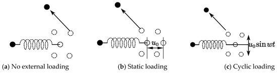
Figure 1.
The thermal disturbance of atomic motion. (a) No external loading; (b) Static loading; (c) Cyclic loading.
As shown in Figure 1b, with the static loading, the critical active energy Q is described as follows:
where is ideal material shear strength, is the external shear stress, is the shear modulus, is the constant associated with stress concentration factor, is the constant associated with the amplitude of the static loading. Combining Equations (1) and (2), the probability of an atom’s active energy above a certain value Q under static loading is described as follows:
where it can be seen that the probability of an atom escaping from the equilibrium position under static loading increased compared with no external loading condition. The displacement u0 of an atom away from the original equilibrium position is invariable. Therefore, the voids generated by the thermal disturbance can be annihilated.
As shown in Figure 1c, with the cyclic loading, the displacement of an atom away from the original equilibrium position is alternating. The voids generated by the thermal disturbance cannot be annihilated so that the damage will be initiated and accumulated.
2.2. Fatigue Damage Evolution Law
The change rate caused by atomic escape is described as follows:
where C is the material constant that contributes to the change rate caused by the probability of atomic escape.
There is a direct correlation between the current stress and the fatigue damage under cyclic loading for the critical energy The damage evolution rate of fatigue under such loading condition is described as follows [52]:
where is cyclic stress amplitude, is mean stress, D is the current damage quantity.
3. Peridynamic Theory for Fatigue Cracking
3.1. Basic Theory
According to peridynamic theory, the physics of a material body at a point interacts with all points within its horizon, as shown in Figure 2. The equation of motion of the material point in the deformed configuration is described as follows [53]:
where is the body load vector, and are the force vector states, is the horizon of point , is the displacement vector at time t.

Figure 2.
The ordinary state-based peridynamic model.
As shown in Figure 2, the bond strain between material points and is described as follows:
As shown in Figure 3, all of the relative position vectors in the horizon of point , is described as follows:
where is the deformation vector state. Equation (8) means that the response of a material point depends collectively on the deformation of all bonds connected to the point.
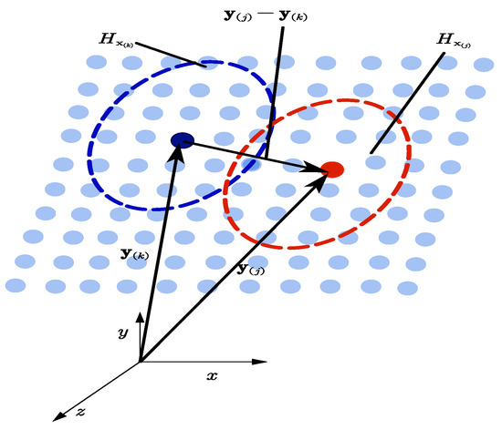
Figure 3.
Deformation vector state .
As shown in Figure 4, the force vector state including an infinite-dimension array force density vectors, , is described as follows:
where the force density vector, , that the material point at location exerts on the material point at location can be expressed as:
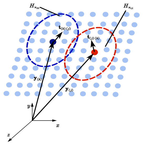
Figure 4.
Force vector state .
As for ordinary state-based peridynamic theory, the scalar state of the force density vector can be expressed as
where is the influence function, is the volume dilatation, is the deviatoric extension state and is the extension scalar state, is the bulk modulus, is the shear modulus, can be expressed respectively as:
where is the elastic modulus, is the Poisson ratio.
For elastic solid material, the strain energy density of material point in the peridynamic state model can be expressed as
where is defined as:
3.2. Energy-Based Failure Criterion
As shown in Figure 5, the force vector states and are opposite in direction and parallel to their deformed relative deformed position. However, their values are not equal.
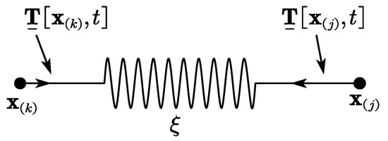
Figure 5.
Force vector state and the bond .
As shown in Figure 6, the force density exhibits non-linearity under cycle loading, therefore the total energy density stored in the bond can be expressed as follows.
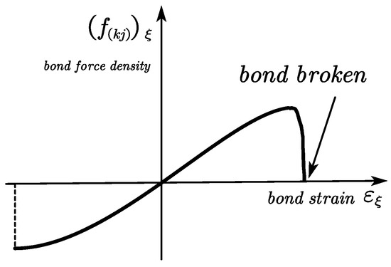
Figure 6.
Critical bond strain damage model.
As shown in Figure 7, all points along the dashed line , connected to all points across fracture plane of unit area and the volume above the fracture plane. The energy density required to open the plane is as follows:
where is the critical energy density, is the energy release rate defined in the continuum damage mechanics theory.

Figure 7.
Fracture surface.
3.3. Fatigue Crack Tip Deformation Analysis
As shown in Figure 8, there are three kinds of bonds near the model-I crack tip: broken bonds, core bonds, and partially damaged bonds. For the core bonds, the bond strain is the largest compared with the partially damaged bonds [46]. Since the material is linear elastic-perfectly plasticity, the core bond strain can be described as:
where is the stress intensity factor, is elastic modulus, is a dimensionless parameter.

Figure 8.
The bonds near the crack tip.
As shown in Figure 9, there is a plastic zone near the crack tip, the length of the plastic zone is . For the linear elastic fracture mechanics, the strain in the plastic zone can be described as:
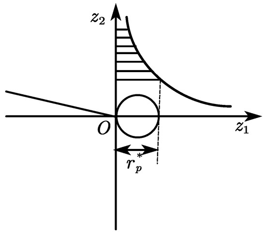
Figure 9.
Plastic zone at fatigue crack tip.
Combining Equations (17) and (18), a function can be described as:
4. Trans-Scale Peridynamic Fatigue Model
In ref. [46], Silling and Askari proposed a fatigue cracking model which can simulate two phases in fatigue failure: crack initiation, crack propagation. The evolution law for the bond “remaining life” is calibrated with S-N curve data during the fatigue crack nucleation phase and with Paris’ law during the fatigue crack growth phase. Inspired by this work, in this section, a trans-scale peridynamic fatigue model is built based on the mechanism of fatigue. Macroscale is directly depicted by the tans-scale peridyanmic model. Each bond in the body is defined as the ideal fatigue test specimen under variable loads.
4.1. Bond Damage and Point Damage within the Horizon
4.1.1. Bond Fatigue Damage and Failure
Bond damage in a peridynamic material body is defined by bond breakage. The simplest criterion is that when the bond strain, shown in Equation (21), exceeds the critical value, the micro-potential between two material points and will be removed away. As shown in Figure 5, the spring-like bond is subjected to variable force density in its two ends during each loading cycle exert on the body . Fatigue bond damage is tracked by a history-dependent variable .
where is the normalized damage function, depending on the current bond strain and time t.
4.1.2. Point Damage and Fatigue Cracking
For a given material point, the point damage is defined as the weighted ratio of the number of eliminated bonds interactions to the total number of initial interactions within its family. The fatigue damage of a point during each loading cycle is described as:
where is an incremental volume for the material point connecting the point within the horizon . As shown in Figure 10, the failure of one bond in the peridynamic body leads to the incremental point damage for and . Therefore, the force density acting among the material points will be redistributed leading to the autonomous damage of neighboring bonds. The progressive failure of bond damage leads to the crack surface in the peridynamic material body.

Figure 10.
The progressive failure in the peridynamic body.
4.2. Trans-Scale Fatigue Model
As shown in Figure 11a,b, The peridynamic solid undergoes cycle loading acting on the body boundary. For a given bond within the horizon of point , the force density acting on the spring-like bond varies in a noncyclic way. The spectrum loading of the bond strain , shown in Figure 11d, varies irregularly with every loading cycle acting on the body boundary. Defines the maximum and minimum bond strains in the current cycle and .
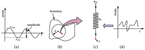
Figure 11.
Fatigue model for a given bond.. (a) Tensile and compress cycle loading; (b) Peridynamic solid; (c) The bond ; (d) Spectrum loading.
As shown in Equation (5), to express the damage accumulation rate of a given bond explicitly, the concise representation of the critical active energy is obtained by using inverse analysis through the damage fatigue failure process and damage fatigue law.
As shown in Figure 12, the normalized fatigue damage quantity can be expressed by fictitious time as follows:
where is the cycle number to failure, is the current cycle number, is the current cycle bond strain in the bond, and are positive parameters corresponding to the material property. The normalized fatigue damage quantity is defined as the consumption life of the bond. It involves the loading cycle increases.
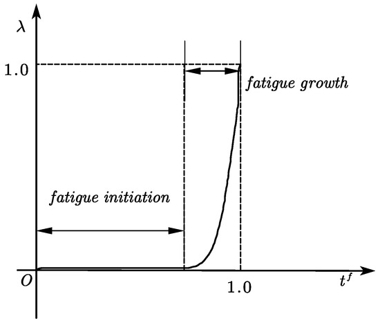
Figure 12.
Scheme of fatigue damage for each bond.
The bond breaks at the loading cycle that
For the fatigue crack initiation phase, parameter and are calibrated by the S-N curve expressed in exponent form, as shown in Figure 13. Equation (25) means that the cycle is the first bond breaks. Parameter and are set to

Figure 13.
Calibration parameters for the initiation phase.
Combining Equations (23), (25) and (26), the first bond in the entire domain breaks with is the cyclic strain range.
where is the smallest cycle at which this bond breaks and . The first bond breaks in the fatigue crack initiation phase when its fatigue cycle number becomes larger than .
When the first bond breaks with the cyclic bond in fatigue crack initiation, new static solutions for other bonds are calculated in the same cycle. If those bonds strain ranges are larger than , then the bonds break and new static solutions continue until no more bonds break at the same cycle. The largest bond strain is calculated for the next cycle number by using the static solution in the deformed peridynamic material configuration.
For the fatigue crack growth phase, parameter and are calibrated by the well-known Paris law. Parameter and are set to
As shown in Figure 14, a fixed bond normal to the axis of the growing model-I fatigue crack. During the cycle loading, the deformation in the vicinity of the crack tip is constant and the crack growth rate is defined as in each loading cycle. The relative distance between the bond and the crack tip is expressed as follows.
where means that the crack tip is on the bond , is the spatial coordinate along the crack axis. The bond consumption life at by integrating its first derivative to distance:
where and , for the damage evolution law is effective within the horizon of the crack tip. Combing Equations (30) and (31) leads to
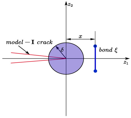
Figure 14.
The bond normal to the model-I crack.
Recall the well-known Paris law for fatigue crack growth:
where and are constant coefficients. Comparing Equations (32) and (33), two experimental data points are selected to determine the constants and .
4.3. Transition from Fatigue Crack Initiation to Growth
As shown in Equation (24), the fatigue crack initiation and growth phase are depicted in a single model. The mechanism of fatigue initiation and growth are different. During the fatigue crack initiation, each bond strain is independent of the cycle number. However, a bond strain is changing over time as the bond transit to the fatigue crack growth phase. As shown in Figure 15, for the given point , within the horizon of point , the bond (denoted as green) transit to the fatigue crack growth phase as the point damage satisfies the following conditions.

Figure 15.
Transition from crack initiation to propagation. (a) Without damage between point and point ; (b) The fatigue crack initiation within the horizon of points and .
5. Numerical Solution Method
5.1. Adaptive Dynamic Relaxation for Static Solution
The peridynamic control equation for fatigue cracking is integral-different. As for cyclic loading simulation, only the maximal loading condition is necessary. Whenever some bonds break in a loading cycle, the new static solution is calculated at the same cycle until no bonds break. To solve quasi-static or static problems, the Adaptive Dynamic Relaxation is used for the fatigue crack simulation problems. The peridynamic equation of motion for all material points is expressed as follows
where is the fictitious diagonal density matrix and is the damping coefficient, and are initial position and displacement vector for all the material points in the configuration body.
where is the number of all the material points in the configuration body. Combing Equations (6) and (11), the vector can be expressed by its component.
where is the total number of material points within the horizon of a material point , is the volume correction factor for the material point . The velocities and displacements for the next time step are expressed as follows.
where is the iteration. The diagonal elements of the density matrix, , can be expressed as:
where is the stiffness matrix of the current structure. As for the small displacement assumption.
where is a unit vector.
5.2. Equivalent Stress Intensity Factor
Each step of crack growth requires a driving force, which guides the fatigue crack path. Naturally, this driving force named stress intensity factor. Because of the complexity in mathematics and physics, solving the three-dimensional dynamic stress intensity factors is certainly limited in mechanics. In the state-based peridynamic theory, there is no concept of this driving force. To better characterize the propagating crack-tip fields, an equivalent stress intensity factor can be expressed as follows [54]:
where , and are 3D Cartesian coordinates with origin at the fatigue crack tip, is a contour integral evaluated counterclockwise along a crack surface, is the traction vector along the crack surface, with the outward unit normal vector and , is a displacement vector and is an element of the crack surface. By taking the surface integration, the relationship between the displacement and fatigue crack criteria is built. Each step of crack growth can be obtained from the relationship.
5.3. Flowchart for the Fatigue Cracking Simulation
Based on the comparison and analysis of the classical fatigue crack simulation algorithm and the peridynamic one, the simulation process for the fatigue crack initiation and growth is deduced, as shown in Figure 16.

Figure 16.
Flowchart of the fatigue cracking simulation.
6. Experiment
6.1. Experimental Equipment
As shown in Figure 17, the experiment was conducted on a fatigue test machine with a floor model biaxial servo-hydraulic dynamic test system, which provides axial and torsion load on a specimen in an integrated biaxial actuator. The system has an axial load capacity of ±250 KN (±56 kip) and a torque capacity of ±2000 Nm (±17700 in-lb), with an axial actuator stroke of 100 mm and a rotary stroke of 90°.
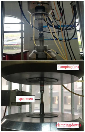
Figure 17.
Fatigue test machine for the combined tension and torsion.
As shown in Figure 18, the loading system, which comes with console software to provide full system control from a personal computer (PC), including waveform generation in both axes, calibration, limit set up, and status monitoring. The loading waveform is sine and the loading frequency is 2HZ.
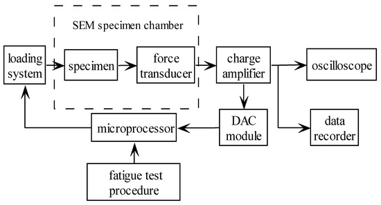
Figure 18.
Hardware configuration of the test system.
6.2. Specimen Size Requirements and Loading Parameters
As shown in Figure 19, a smooth specimen with a length of 210 mm is machined cutting from a high-speed wheel. The diameter of the grasping side is 25 mm. The minimum diameter of the test specimen is 7 mm, which also means that it is the weak part of the specimen without considering other factors. The maximum percentages of the various specified elements are shown in Table 1. The basic mechanical properties for the wheel material are shown in Table 2. The loading parameters are shown in Table 3 and the loading path is shown in Figure 20.
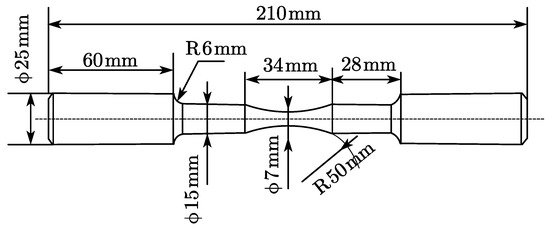
Figure 19.
Fatigue specimen.

Table 1.
The maximum percentages of the various specified elements.
Table 2.
Basic properties of the wheel material at room temperature.
Table 3.
Loading parameters.
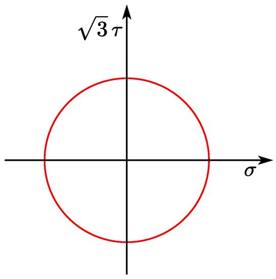
Figure 20.
Loading path.
6.3. Fatigue Crack Path and Morphology
The fracture morphology and the angle between the fatigue crack path and the central axis are shown in Figure 21.
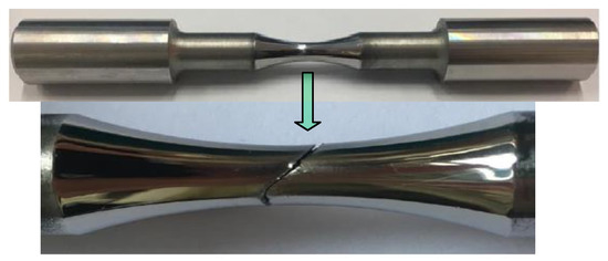
Figure 21.
Macro fracture characteristics of the smooth specimen.
6.4. Results Analysis
As shown in Figure 22, using an electron microscope, it can be seen that the angle between the main long fatigue crack and cylinder axis line is about °.
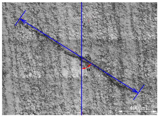
Figure 22.
The angle and morphology of fatigue crack.
As shown in Table 4, the average fatigue cycle is 15,992 for the fatigue specimens, and the average angle between the main long fatigue crack and cylinder axis line is 61.54°.
Table 4.
Fatigue cycles and angles.
As shown in Figure 23, the angle between the main long fatigue crack and cylinder axis line is about 58.5°. This simulation result has a good correlation with the average test result, as shown in Figure 22.
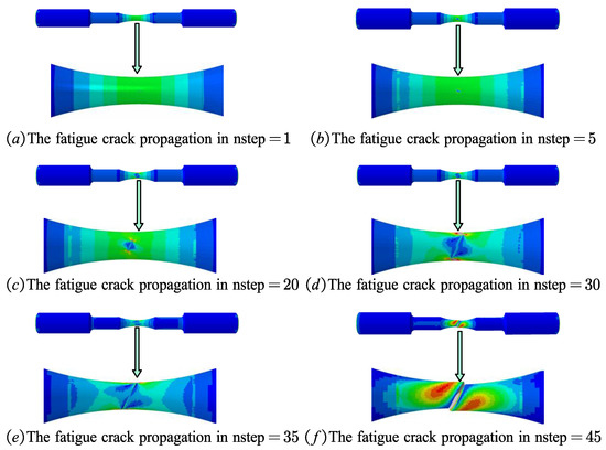
Figure 23.
Simulation results based on the proposed peridynamic fatigue model. (a) The fatigue crack propagation in ; (b) The fatigue crack propagation in ; (c) The fatigue crack propagation in ; (d) The fatigue crack propagation in ; (e) The fatigue crack propagation in ; (f) The fatigue crack propagation in .
As shown in Figure 24, the value of the equivalent stress intensity factor becomes larger as the number of iterations increases.
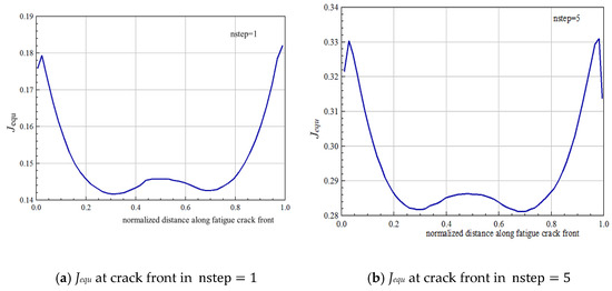
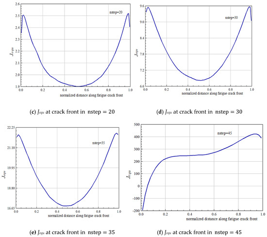
Figure 24.
Equivalent stress intensity factors in each specified iteration. (a) Jequ at crack front in ; (b) Jequ at crack front in ; (c) Jequ at crack front in ; (d) Jequ at crack front in ; (e) Jequ at crack front in ; (f) Jequ at crack front in .
7. Conclusions
- (1)
- To evaluate and predict the fatigue life of specimens under combined tension and torsion, the peridynamic fatigue model was proposed and the fatigue cracks initiate and propagate naturally without extra criteria.
- (2)
- The proposed trans-scale fatigue model has no notion of scale, or it releases the scale constraints. The evolution of fatigue crack shows micro and macro scale including crack initiation, propagation, and fracture.
- (3)
- The short diffusion-generated and propagating crack converges and grows into the main crack, which expands to the macroscopic visible morphology.
- (4)
- The macroscopic morphology of fatigue was highly consistent with the actual experimental results and extended along the direction of 61.54° until the final fracture.
- (5)
- The natural propagation of the crack can be realized without the need for additional crack propagation criteria, and the distribution and quantitative analysis of the fatigue life can be obtained.
Author Contributions
Conceptualization, W.C.; methodology, J.H. and W.C.; formal analysis, J.H. and W.C.; investigation, W.C.; resoures, J.H. and W.C.; writing-original draft preparation, J.H. and W.C.; writing-review and editing, J.H. and W.C.; visualization, J.H.; supervision, W.C.; funding acquisition, W.C.; All authors have read and agreed to the published version of the manuscript.
Funding
This research was partially supported by the Joint Funds of the National Natural Science Foundation of China (Grant No. U1334204).
Conflicts of Interest
The author(s) declared no potential conflicts of interest with respect to the research, authorship, and/or publication of this article.
References
- Klesnil, M.; Lukác, P. Fatigue of Metallic Materials; Elsevier: Amsterdam, The Netherlands, 1992. [Google Scholar]
- Bannantine, J.; Comer, J.; Handrock, J. Fundamentals of Metal Fatigue Analysis((Book)); Research Supported by the University of Illinois Englewood Cliffs: Prentice Hall, NJ, USA, 1990; Volume 286. [Google Scholar]
- Schijve, J. Fatigue of Structures and Materials; Springer Science & Business Media: New York, NY, USA, 2001. [Google Scholar]
- Antonopoulos, J.G.; Brown, L.M.; Winter, A.T. Vacancy dipoles in fatigued copper. Philos. Mag. 1976, 34, 549–563. [Google Scholar] [CrossRef]
- Man, J.; Obrtlik, K.; Blochwitz, C.H.; Polak, J. Atomic force microscopy of surface relief in individual grains of fatigued 316L austenitic stainless steel. Acta Mater. 2002, 50, 3767–3780. [Google Scholar] [CrossRef]
- Brinckmann, S.; Sivanesapillai, R.; Hartmaier, A. On the formation of vacancies by edge dislocation dipole annihilation in fatigued copper. Int. J. Fatigue 2011, 33, 1369–1375. [Google Scholar] [CrossRef]
- Oskay, C.; Fish, J. Fatigue life prediction using 2-scale temporal asymptotic homogenization. Int. J. Numer. Methods Eng. 2004, 61, 329–359. [Google Scholar] [CrossRef]
- Vinogradov, A.; Hashimoto, S. Multiscale phenomena in fatigue of ultra-fine grain materials—An overview. Mater. Trans. 2001, 42, 74–84. [Google Scholar] [CrossRef]
- Fish, J.; Bailakanavar, M.; Powers, L.; Cook, T. Multiscale fatigue life prediction model for heterogeneous materials. Int. J. Numer. Methods Eng. 2012, 91, 1087–1104. [Google Scholar] [CrossRef]
- Lépinoux, J.; Mazière, D.; Pontikis, V.; Saada, G. Multiscale Phenomena in Plasticity: From Experiments to Phenomenology, Modelling and Materials Engineering; Springer Science & Business Media: Ouranoupolis, Greece, 2012. [Google Scholar]
- Oskay, C.; Fish, J. Multiscale modeling of fatigue for ductile materials. Int. J. Multiscale Comput. Eng. 2004, 2. [Google Scholar] [CrossRef]
- Jung, J.; Seok, J. Fatigue crack growth analysis in layered heterogeneous material systems using peridynamic approach. Compos. Struct. 2016, 152, 403–407. [Google Scholar] [CrossRef]
- Hanson, M.T.; Keer, L.M. An analytical life prediction model for the crack propagation occurring in contact fatigue failure. Tribol. Trans. 1992, 35, 451–461. [Google Scholar] [CrossRef]
- Yang, B.; Mall, S.; Ravi-Chandar, K. A cohesive zone model for fatigue crack growth in quasibrittle materials. Int. J. Solids Struct. 2001, 38, 3927–3944. [Google Scholar] [CrossRef]
- Pook, L. Why Metal Fatigue Matters; Springer: Berlin/Heidelberg, Germany, 2007. [Google Scholar]
- Schijve, J. Fatigue damage in aircraft structures, not wanted, but tolerated? Int. J. Fatigue 2009, 31, 998–1011. [Google Scholar] [CrossRef]
- Liu, Y.; Mahadevan, S. Multiaxial high-cycle fatigue criterion and life prediction for metals. Int. J. Fatigue 2005, 27, 790–800. [Google Scholar] [CrossRef]
- Nisitani, H.; Teranishi, T. KI of a circumferential crack emanating from an ellipsoidal cavity obtained by the crack tip stress method in FEM. Eng. Fract. Mech. 2004, 71, 579–585. [Google Scholar] [CrossRef]
- Kikuchi, M.; Wada, Y.; Shintaku, Y.; Suga, K.; Li, Y. Fatigue crack growth simulation in heterogeneous material using s-version FEM. Int. J. Fatigue 2014, 58, 47–55. [Google Scholar] [CrossRef]
- Ondráček, J.; Materna, A. FEM evaluation of the dissipated energy in front of a crack tip under 2D mixed mode loading condition. Procedia Mater. Sci. 2014, 3, 673–678. [Google Scholar] [CrossRef][Green Version]
- Solanki, K.; Daniewicz, S.R.; Newman, J.C., Jr. Finite element analysis of plasticity-induced fatigue crack closure: An overview. Eng. Fract. Mech. 2004, 71, 149–171. [Google Scholar] [CrossRef]
- Sukumar, N.; Chopp, D.L.; Moran, B. Extended finite element method and fast marching method for three-dimensional fatigue crack propagation. Eng. Fract. Mech. 2003, 70, 29–48. [Google Scholar] [CrossRef]
- Anahid, M.; Samal, M.K.; Ghosh, S. Dwell fatigue crack nucleation model based on crystal plasticity finite element simulations of polycrystalline titanium alloys. J. Mech. Phys. Solids 2011, 59, 2157–2176. [Google Scholar] [CrossRef]
- Roe, K.L.; Siegmund, T.H. An irreversible cohesive zone model for interface fatigue crack growth simulation. Eng. Fract. Mech. 2003, 70, 209–232. [Google Scholar] [CrossRef]
- Newman, J.C. A crack-closure model for predicting fatigue crack growth under aircraft spectrum loading. In Methods and Models for Predicting Fatigue Crack Growth under Random Loading; ASTM International: West Conshohocken, PA, USA, 1981. [Google Scholar]
- Nguyen, O.; Repetto, E.A.; Ortiz, M.; Radovitzky, R.A. A cohesive model of fatigue crack growth. Int. J. Fract. 2001, 110, 351–369. [Google Scholar] [CrossRef]
- Giner, E.; Sukumar, N.; Tarancón, J.E.; Fuenmayor, F.J. An Abaqus implementation of the extended finite element method. Eng. Fract. Mech. 2009, 76, 347–368. [Google Scholar] [CrossRef]
- Pathak, H.; Singh, A.; Singh, I.V. Fatigue crack growth simulations of 3-D problems using XFEM. Int. J. Mech. Sci. 2013, 76, 112–131. [Google Scholar] [CrossRef]
- Bergara, A.; Dorado, J.I.; Martin-Meizoso, A.; Martínez-Esnaola, J.M. Fatigue crack propagation in complex stress fields: Experiments and numerical simulations using the Extended Finite Element Method (XFEM). Int. J. Fatigue 2017, 103, 112–121. [Google Scholar] [CrossRef]
- Kumar, S.; Shedbale, A.S.; Singh, I.V.; Mishra, B.K. Elasto-plastic fatigue crack growth analysis of plane problems in the presence of flaws using XFEM. Front. Struct. Civ. Eng. 2015, 9, 420–440. [Google Scholar] [CrossRef]
- Bhattacharya, S.; Singh, I.V.; Mishra, B.K.; Bui, T.Q. Fatigue crack growth simulations of interfacial cracks in bi-layered FGMs using XFEM. Comput. Mech. 2013, 52, 799–814. [Google Scholar] [CrossRef]
- Xu, Y.; Yuan, H. On damage accumulations in the cyclic cohesive zone model for XFEM analysis of mixed-mode fatigue crack growth. Comput. Mater. Sci. 2009, 46, 579–585. [Google Scholar] [CrossRef]
- Sangid, M.D. The physics of fatigue crack initiation. Int. J. Fatigue 2013, 57, 58–72. [Google Scholar] [CrossRef]
- Fu, H.-H.; Benson, D.J.; Meyers, M.A. Analytical and computational description of effect of grain size on yield stress of metals. Acta Mater. 2001, 49, 2567–2582. [Google Scholar] [CrossRef]
- Al-Rub, R.K.A.; Voyiadjis, G.Z. On the coupling of anisotropic damage and plasticity models for ductile materials. Int. J. Solids Struct. 2003, 40, 2611–2643. [Google Scholar] [CrossRef]
- Shenoy, M.M.; Gordon, A.P.; Mcdowell, D.L.; Neu, R.W. Thermomechanical fatigue behavior of a directionally solidified Ni-base superalloy. J. Eng. Mater. Technol. 2005, 127, 325–336. [Google Scholar] [CrossRef]
- Lemaitre, J.; Chaboche, J.-L. Mechanics of Solid Materials; Cambridge University Press: Cambridge, UK, 1994. [Google Scholar]
- Wilsdorf, H.G.F. The ductile fracture of metals: A microstructural viewpoint. Mater. Sci. Eng. 1983, 59, 1–39. [Google Scholar] [CrossRef]
- Silling, S.A.; Lehoucq, R.B. Peridynamic Theory of Solid Mechanics. In Advances in Applied Mechanics; Elsevier: Amsterdam, The Netherlands, 2010; pp. 73–168. [Google Scholar]
- Madenci, E.; Oterkus, E. Peridynamic Theory and Its Applications; Springer: New York, NY, USA, 2014. [Google Scholar]
- Kilic, B.; Agwai, A.; Madenci, E. Peridynamic theory for progressive damage prediction in center-cracked composite laminates. Compos. Struct. 2009, 90, 141–151. [Google Scholar] [CrossRef]
- Seleson, P.; Parks, M. On the role of the influence function in the peridynamic theory. Int. J. Multiscale Comput. Eng. 2011, 9, 689–706. [Google Scholar] [CrossRef]
- Kilic, B.; Madenci, E. Structural stability and failure analysis using peridynamic theory. Int. J. Non-Linear Mech. 2009, 44, 845–854. [Google Scholar] [CrossRef]
- Kilic, B.; Madenci, E. Prediction of crack paths in a quenched glass plate by using peridynamic theory. Int. J. Fract. 2009, 156, 165–177. [Google Scholar] [CrossRef]
- Oterkus, E.; Guven, I.; Madenci, E. Fatigue failure model with peridynamic theory. In Proceedings of the 2010 12th IEEE Intersociety Conference on Thermal and Thermomechanical Phenomena in Electronic Systems, F, 2010 IEEE, Las Vegas, NV, USA, 2–5 June 2010. [Google Scholar]
- Silling, S.A.; Askari, A. Peridynamic Model for Fatigue Cracking; Sandia National Laboratories: Albuquerque, NM, USA, 2014. [Google Scholar]
- Sarego, G.; Le Quang, V.; Bobaru, F.; Zaccariotto, M.; Galvanetto, U. Linearized state-based peridynamics for 2-D problems. Int. J. Numer. Methods Eng. 2016, 108, 1174–1197. [Google Scholar] [CrossRef]
- Zhang, G.; Le, Q.; Loghin, A.; Subramaniyan, A.; Bobaru, F. Validation of a peridynamic model for fatigue cracking. Eng. Fract. Mech. 2016, 162, 76–94. [Google Scholar] [CrossRef]
- Baber, F.; Guven, I. Solder joint fatigue life prediction using peridynamic approach. Microelectron. Reliab. 2017, 79, 20–31. [Google Scholar] [CrossRef]
- Littlewood, D.J. A nonlocal approach to modeling crack nucleation in AA 7075-T651. In Proceedings of the ASME 2011 International Mechanical Engineering Congress and Exposition, Denver, CO, USA, 11–17 November 2011; pp. 567–576. [Google Scholar]
- Hu, Y.L.; Madenci, E. Peridynamics for fatigue life and residual strength prediction of composite laminates. Compos. Struct. 2017, 160, 169–184. [Google Scholar] [CrossRef]
- Yokobori, T. The Strength, Fracture, and Fatigue of Materials; P. Noordhoff: Groningen, The Netherlands, 1965. [Google Scholar]
- Silling, S.A.; Epton, M.; Weckner, O.; Xu, J.; Askari, E. Peridynamic States and Constitutive Modeling. J. Elast. 2007, 88, 151–184. [Google Scholar] [CrossRef]
- Stenström, C.; Eriksson, K. The J-contour integral in peridynamics via displacements. Int. J. Fract. 2019, 216, 173–183. [Google Scholar] [CrossRef]


© 2020 by the authors. Licensee MDPI, Basel, Switzerland. This article is an open access article distributed under the terms and conditions of the Creative Commons Attribution (CC BY) license (http://creativecommons.org/licenses/by/4.0/).