Effect of Liquid Viscosity and Flow Orientation on Initial Waves in Annular Gas–Liquid Flow

Abstract

The complex wave structure of annular gas–liquid flow with disturbance waves and liquid entrainment is a result of the evolution of high-frequency initial waves, appearing at the very inlet of the flow, prior to the hydrodynamic stabilization of liquid film. This stage of flow evolution is studied experimentally, using a shadow technique, and theoretically, using a linear stability analysis of the Orr–Sommerfeld equation in both phases. The present work is focused on the comparison of earlier results obtained in air–water downward flow with the new results obtained in upward flow and with more viscous liquids. The flow orientation affects the shape of the liquid film prior to stabilization; the initial film area is thicker but shorter in upward flow. Upward flow orientation also leads to a lower frequency and the increment of growth of initial waves. The viscosity effect is found to be weak if flow rates of both phases are the same. The model is mostly able to reproduce the qualitative trends, but the quantitative agreement is not reached. Experimental observations indicate that the liquid flow within the initial area is significantly different from the stabilized flow of gas-sheared liquid film, which is used in the model. This difference could explain the discrepancy; further development of the model should be aimed at taking into account the evolution of the velocity profile inside the liquid film during the stage of hydrodynamic stabilization.

1. Introduction

An annular flow pattern is observed when a gas–liquid mixture with a high fraction of gas phase flows in a duct. This flow is characterized by existence of a continuous gas core and a continuous liquid film on the duct walls. The dispersed phase consists of liquid droplets torn from the film surface and entrained into the gas core, and the gas bubbles are entrapped by the liquid film. Annular flow occurs in many industrial and power applications such as heat exchangers, steam generators, absorbers, oil-and-gas pipelines, as well as nuclear reactors. The efficiency and safety of the operation of these facilities demand a prediction of the overall flow characteristics, including the pressure drop, film thickness, entrained fraction, heat transfer and the critical heat flux. At present, the predictions are based on empirical correlations, which simplify the flow physics significantly. The interaction of the gas stream and liquid film leads to the creation of a complex system of waves on the film surface. The dominant structures in this system are so-called disturbance waves, which are large lumps of liquid traveling with a high speed over a thin residual layer of liquid (“base film”). The disturbance waves generate small-scale ripple waves which propagate over both the base film and disturbance waves. Both disturbance waves and ripples affect the interfacial shear, the mixing of liquid, heat transfer and turbulence in both phases; they are necessary for the entrainment of liquid and gas entrainment. Physical modeling of integral flow parameters requires the modeling of disturbance waves and ripples as a necessary first step.

The properties of disturbance waves and ripples were measured in many experimental works. It is well known that the average velocity and frequency of the disturbance waves grow linearly with the superficial gas velocity, whilst the height of the waves decreases with gas speed, along with film thickness in general [1,2,3,4]. An increase in liquid flow rate leads to an increase in all the aforementioned characteristics. The properties of the waves are affected by many other parameters, such as duct shape [5] and hydraulic diameter [6,7,8], flow orientation [9], liquid viscosity [10,11] and surface tension [12,13,14], gas density [15,16,17], etc. However, apart from empirical approaches with their obvious limitations [18,19,20,21], the prediction of wave properties by numerical or semi-analytical models is far from successful yet. One of the problems with modeling is that the wave structure of the liquid film is also affected by the distance from the point of primary contact between the phases. Even if the entrance of liquid is smooth—i.e., when the liquid is introduced as a film from the very beginning—the film undergoes a cascade of qualitative and quantitative changes. It is hardly possible to produce a working model which ignores the stage of flow development. At least, the numerical model with a long computational domain starting from the inlet [22] reproduces the experimental characteristics of disturbance waves much better than those employing periodic boundary conditions in the flow direction (e.g., [23,24]). In general, a disturbance wave should be modeled starting from an infinitesimal perturbation near the inlet, passing through all the stages of evolution observed in the experiments. Those stages are described below. Very close to the inlet, the film surface is smooth; high-frequency initial waves appear here and grow in amplitude as they propagate downstream. Further downstream coalescence of the initial waves leads to the formation of large-scale disturbance waves which produce ripples on their rear slopes [25]. The disturbance waves coalesce with each other, which reduces their frequency with downstream distance [26,27], whilst their velocity grows downstream [28]. It takes a distance of order of 100 pipe diameters to reach relatively stabilized waves properties [28].

The main idea of our recent paper [29] was that the modeling of waves in annular flow had to consecutively deal with all the stages of the waves’ evolution and be conducted in close relation to the experiments. The paper was focused on the investigation of the initial waves and liquid film at this stage of evolution. It was found that, after the film leaves the inlet slot, its thickness is comparable to that of the slot, until it abruptly falls to a much thinner value. The initial waves appear and grow on this “thick” film. They were found to be two-dimensional and surprisingly regular in the absence of external perturbations; both characteristics were lost when the film thickness dropped to the “equilibrium” value.

The main parameters of the liquid film and initial waves were measured with the shadow method. The length of the initial area was found to increase with the liquid flow rate and decrease with gas velocity. Frequency, velocity and the increment of the amplitude growth of the initial waves were measured and compared to the properties of the waves of maximum growth predicted in frames of linear stability analysis. The velocity of the waves was predicted reasonably well. The predicted frequency of the waves corresponded well to the experiments for the moderate liquid flow rates, but for larger flow rates, the modeled values exceed the measured ones. The increment of amplitude growth is significantly underestimated by the model, so further development of the models is necessary.

The results described above were obtained for downward air–water annular flow. As mentioned above, many parameters affect the liquid film and its wave structure. In the present paper, we aim at expanding the range of conditions within the same problem statement. We investigate the effect of flow orientation by comparing the initial waves in upwards and downwards flows and the effect of liquid viscosity by using water–glycerol solutions as working liquids.

2. Materials and Methods

The annular flow was organized in a vertical acrylic resin pipe with an inner diameter D = 11.7 mm and a wall thickness of 10 mm. Prior to the experiments, the working liquid was pumped from the receiving tank into the pressure tank, located 3 m above the inlet. After that, the pump was switched off and the liquid flowed under the static pressure. The liquid flow rate was controlled by a float rotameter. The distributor vessel with a volume of about 1 L was filled with working liquid. From there the liquid was fed into the working section through a ring-shaped slot with a thickness of 0.5 mm between the inner wall of the pipe and the gas-feeding tube (the tube’s wall thickness is 0.3 mm). The latter was mounted coaxially with the pipe; the gas was supplied from a centralized line of compressed air. The gas flow was controlled using an orifice meter. Thus, the liquid was introduced as a film and the annular flow started from the inlet. At the outlet, the gas–liquid mixture was separated so that the liquid returned to the receiving tank and the gas was thrown into the atmosphere.

The scheme of the inlet is shown in Figure 1a for the case of a downward flow. Upward flow can be organized easily by literally turning the whole working section with the distributor and separator upside down. If the gas flow is strong enough, it will drag the liquid film upwards. Preliminary tests have shown that no liquid flows downwards in an upward flow configuration for superficial gas velocities over 15 m/s for the whole range of liquid flow rates employed. In both downward and upwards configurations, the range of superficial gas velocities, V_G, is from 15 to 50 m/s with a step of 7 m/s.

Three working liquids were used: water and two water–glycerol solutions with a mass concentration of glycerol of 20% and 33% (WGS1 and WGS2, respectively). The values of kinematic viscosity of the liquids, v, are 1.15, 2 and 3 cSt (10⁻⁶ m²/s), respectively. The viscosity was measured with a capillary viscosimeter at working temperature, which was about 16 °C for all cases. The error of the viscosity measurements did not exceed 2%. The surface tension of the glycerol solutions was only slightly lower than that of water, so its effect may be neglected.

Liquid flow rates for water were selected to correspond to the liquid film Reynolds numbers of 140, 220 and 300, which were employed in [29]. The liquid Reynolds number is defined as:

$$R{e}_L=\frac{Q}{\pi D\upsilon },$$

(1)

where Q is the volumetric liquid flow rate. For the water–glycerol solutions, flow rates corresponding to the same Re_L were used. However, for WGS2, another set of liquid flow rates was used in addition to the same volumetric flow rates as for water.

The measurements of local instantaneous film thickness were conducted using the shadow technique, used, e.g., in [21,30]. In the present paper, we employed the same configuration as used in [29]. The detailed methodical analysis of the technique can be found in that paper; here, a brief description of its principles is given. The pipe was illuminated by a white lamp through a diffusing screen for more uniform illumination. The light passing through the pipe was registered by a high-speed camera located on the opposite side of the pipe. If a ray passes through the pipe wall and liquid film without “touching” the gas–liquid interface, it illuminates a particular pixel of the camera. If a ray crosses the interface, it is refracted/reflected (in the area we are looking at, it will be, as a rule, the total internal reflection) and the corresponding pixel will remain dark. Based on the transverse size of the bright area in the camera image (see the top part of Figure 1b and the bottom parts of all the subfigures of Figure 2 for examples of instantaneous thickness profiles), the local film thickness can be measured at each downstream position. This method would underestimate the amplitude of three-dimensional waves; however, the initial waves under study were proven to be essentially two-dimensional [29]. Combining instantaneous spatial records of film thickness, h(x), one receives a spatiotemporal matrix, h(x,t). An example of such a matrix in graphical representation is shown in Figure 1b. The brightness of each pixel of this image is directly proportional to the film thickness value in a corresponding cell of h(x,t) matrix; white corresponds to h = 1 mm. The spatial resolution of the technique in the longitudinal direction is 40 µm per pixel; in the radial direction, spatial resolution is 30 µm/pixel due to magnification of the image at the outer wall of the pipe. The sampling frequency is 10 kHz; for each set of conditions, at least one record with duration of 1 s was obtained.

3. Result

The investigation of the initial stage of film evolution consists of two main parts: studying the shape the film takes at this stage and the characteristics of the waves, generated and growing during this stage. The two parts will be considered in Section 3.1 and Section 3.2; a comparison of the wave characteristics to the model prediction will be given in Section 3.3.

3.1. The Film Shape at the Initial Stage

Inside the distributor slot, the liquid flow can be described by a symmetric parabolic velocity profile. The liquid is accelerated by the hydrostatic pressure exerted by the liquid in the pressure tank and decelerated by viscous friction at the slot walls, modeled by the no-slip condition at both walls. Far from the outlet, a semi-parabolic profile of liquid velocity is expected. The liquid is accelerated by the interfacial shear force exerted by the gas stream and decelerated by viscous friction at the pipe inner wall. Gravity may either accelerate or decelerate the flow depending on flow orientation.

The transition from one state to the other requires a certain time and consequently, the distance for the liquid to travel. The thickness of the liquid film changes with a downstream distance from the slot thickness at the slot outlet to the “equilibrium” value far from the slot, which depends on the balance between the gas drag force, gravity, liquid inertia, and viscous friction. For thin liquid films, the thickness decreases rapidly at the beginning, then decays exponentially; see, e.g., Figure 2c in [29], where the thickness of the liquid film at Re_L = 30 flowing downwards in absence of gas flow is investigated. For thicker water films flowing downwards, it was found in the same paper that the film thickness is kept on a relatively constant level, close to the thickness of the slot, for a certain distance and then undergoes rapid decrease to the “equilibrium” value. The length of the “thick” film was found to grow with a liquid flow rate and decrease with gas velocity.

Examples of the time-averaged profiles of film thickness along a downstream coordinate are shown in the top parts of subfigures in Figure 2 as blue and red lines for the downward and upward flow, respectively. Examples of raw instantaneous frames with superimposed interface positions are given in the bottom parts of each subfigure; the frame for the downward flow is above the one for the upward flow. For the downward flow, the shape of the initial film is a relatively long plateau of a film with a thickness slightly larger than that of the slot (0.5 mm); further downstream, the thickness drops to a thinner “equilibrium” value. In the case of upward flow, the film gets noticeably thicker than the slot just after the slot outlet (Figure 2a). On the other hand, this “thick film” stage is much shorter than in a downward flow. When the gas superficial velocity is high (Figure 2b), the difference between the upward and downward flows becomes less pronounced: the transition to the “equilibrium” film stage occurs at nearly the same downstream distance, and at the initial stage the film is only slightly thicker in upward flow.

To analyze the effect of flow conditions on the film shape at the initial stage, two parameters were measured: maximum time-averaged film thickness, H_max, and the distance at which the “equilibrium” film thickness is reached, X. Figure 3 shows the behavior of H_max for different conditions. There is a prominent effect of flow orientation. In upward flow, H_max decreases with V_G. At the lowest V_G = 15 m/s it even exceeds the joint thickness of the slot (0.5 mm) and the gas-feeding tube (0.3 mm), thus protruding by 0.1–0.2 mm into the gas core. At a larger V_G, H_max is smaller than 0.8 mm and gets close to the slot thickness at the largest V_G. In upward flow, the gravity assists the accumulation of liquid behind the slot outlet. The gas drag is strong enough to prevent the liquid from flowing down the dry inner side of the gas-feeding tube, so the liquid is gathered in the “pocket” on top of the end of the gas-feeding tube. The higher V_G is, the stronger is the gas resistance to the spreading of liquid over this narrow surface.

In downward flow, gravity prevents the accumulation of liquid downstream from the slot outlet, and no strong local thickening of the liquid film occurs. H_max is slightly (10–20%) larger than the slot thickness and it does not show any strong dependence on V_G. Moreover, in both upward and downward flow, H_max is independent on the liquid flow rate. This film thickness behavior is quite different from that of stabilized gas-sheared liquid films, where film thickness increases with liquid flow rate and decreases with gas velocity in either upward or downward flow.

However, the gas and liquid flow rates strongly affect the length of the stabilization zone, X. The results of the measurements are presented in Figure 4. With increasing V_G, X decreases approximately as $V_G^{-2}$ (see Figure 4a,b). With an increasing liquid flow rate, X increases. In the same subfigures, a comparison between the liquids with different viscosities is presented. Despite almost threefold viscosity difference, the length of the stabilization zone is almost the same at the same volumetric flow rate of the liquid. If the same liquid Reynolds numbers were compared, the liquid flow rate would have been almost three times larger for WGS2, along with the X value. This implies the independence of X on liquid viscosity at a fixed Q, which is quite surprising.

In downward flow, the X values are larger than in the upward flow if other conditions are the same. The quantitative effect of flow orientation is shown in Figure 4c, where the direct comparison is given. Obviously, the largest values correspond to the lowest V_G and the largest Q_L, and vice versa; the values X > 40 mm (i.e., the cases when stabilization is not reached within the interrogation area) are not shown. In general, X is about 20% lower in the upward flow; at the largest V_G, the difference nearly disappears.

The same trend can be seen in Figure 4d, where the dependence of X on the liquid flow rate at a fixed gas velocity is shown. It includes all the experimental points with V_G = 29 m/s in an upward/downward flow for all three working liquids. All the points lie around the same line, further supporting the idea of independence of X on viscosity.

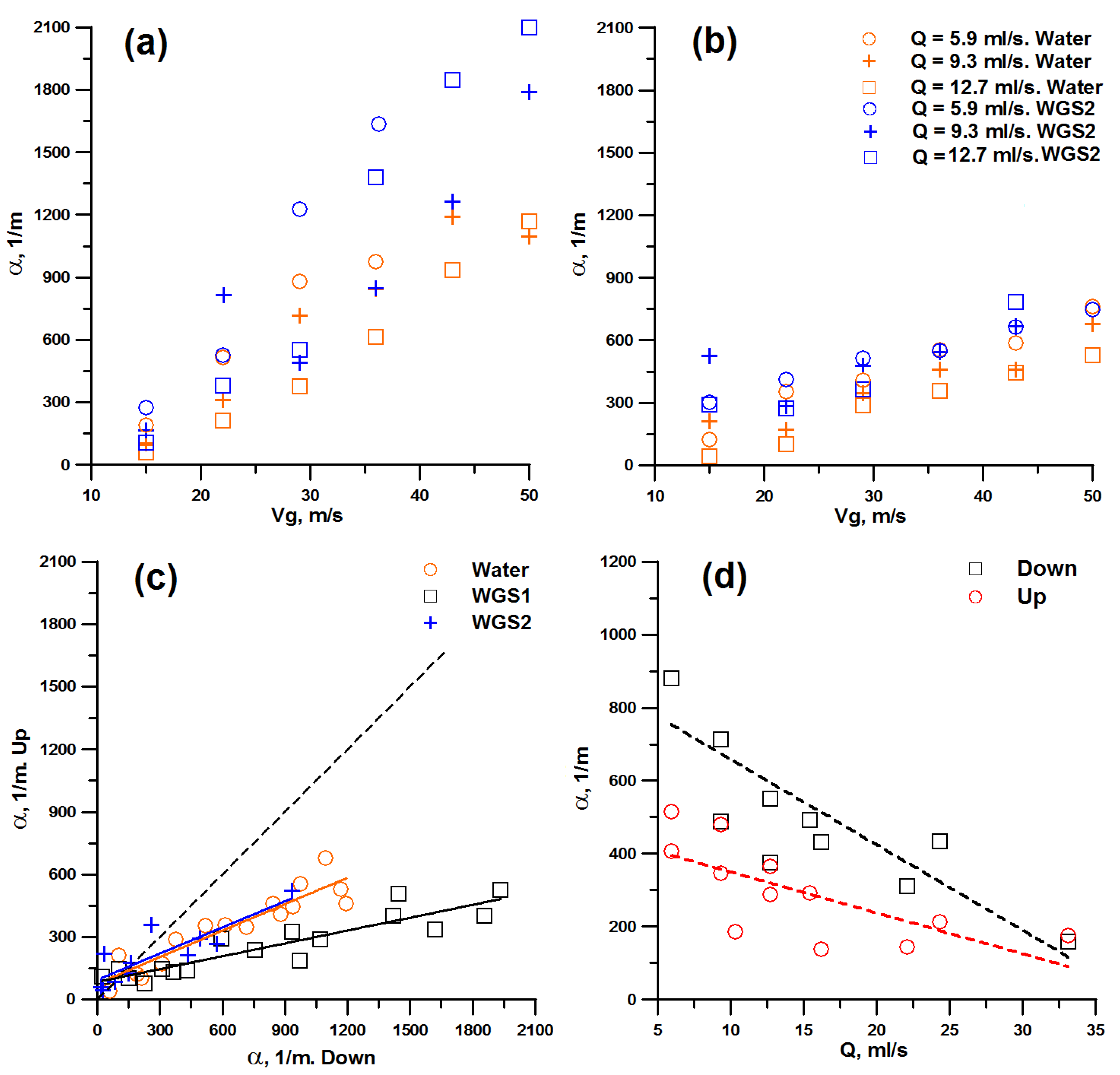
3.2. Characteristics of the Initial Waves

As mentioned above, the initial waves appear and grow on top of the “thick” initial film, prior to the stabilization of film thickness. These waves can be approximately described by the equation of a running sinusoidal wave with exponentially growing amplitude, namely:

$$h\left(x,t\right)=h_0\left(x\right)+A_0\ast \exp \left(ikx-ikct+\alpha x\right)$$

(2)

where h₀ is local time-averaged film thickness, A₀ is wave amplitude at x = 0, k is the wavenumber, c is the phase velocity and α is the spatial increment of amplitude growth. Three main parameters of the waves which can be measured to characterize them are the frequency (f = kc/2π), velocity, and increment. The frequency is measured by a direct counting algorithm applied to the temporal records of film thickness within the distance range corresponding to the appearance and growth of initial waves on the thick film. The algorithm identifies parts of the record when h(x_i,t) is larger or lower than h₀(x_i). The median value of the duration of adjacent pairs of such “crest” and “trough” parts of waves is taken as a wave period and used to calculate the frequency. The total frequency was estimated as the median over all the “local” values within the area of existence of initial waves.

The results of frequency measurements are presented in Figure 5 in the same manner as used previously for X in Figure 4. Frequency shows a prominent, approximately linear, growth with gas velocity and a weaker growth with the liquid flow rate (Figure 5a,b). There is also a minor effect of liquid viscosity: larger viscosity results in slightly higher frequencies at the same liquid flow rate. The viscosity effect is stronger in the case of upward flow and larger liquid flow rates.

The frequency values are larger in downward flow if all the other conditions are the same (Figure 5c). In this Figure, the largest frequency values correspond to the largest gas and liquid flow rates; in this area, the strongest deviations from the average line are observed. At moderate gas velocities, the frequency shows linear growth with a liquid flow rate, and the data for the liquids with different viscosities lie on quite the same straight lines (Figure 5d). The difference between the frequencies of the initial waves in the upward and downward flows increases with the liquid flow rate.

Velocities of the waves were measured based on the time delay between the temporal records obtained at different downstream coordinates determined by the position of maximum in cross-correlation function between the two records. The measurement results are shown in Figure 6. The wave velocity is nearly independent on gas velocity (Figure 6a,b), which is, again, unusual for waves on gas-sheared liquid films. It grows with the liquid flow rate, but there is no noticeable effect of viscosity or flow orientation. The absence of any strong orientation effect is also demonstrated in Figure 6c,d. The velocity grows linearly with a liquid flow rate and, as in the case of stabilization length and frequency, the data for different viscosity lie on the same line.

The amplitude of the waves at a fixed downstream distance is identified as the standard deviation of a temporal record. This value is several times smaller than the peak-to-peak amplitude of the signal, but it can be used for the estimation of the spatial increment of amplitude growth. The latter is defined as the logarithm of the ratio of amplitudes, and it is assumed that the shape of the waves does not change significantly during the short distance so that the ratio of peak-to-peak amplitude to standard deviation remains the same.

In general, the measured values of increment show a much larger uncertainty than those of frequency or velocity. This could be expected since a relatively small change of amplitude has to be detected over a very short length. The discretized character of the film thickness values increases uncertainty even further. However, general trends can be identified in the same manner as for other characteristics of the waves (Figure 7).

The increments grow with gas velocity; larger viscosity at the same liquid flow rate yields larger increments (Figure 7a,b). In contrast to velocity and frequency, the increments are lower at larger liquid flow rates. In upward flow, wave growth is much slower than in downward flow (Figure 7c). It is interesting that the effect of flow orientation is stronger at larger gas velocities and lower liquid flow rates. Figure 7d shows a strong decrease in the increment with a liquid flow rate at a constant gas velocity.

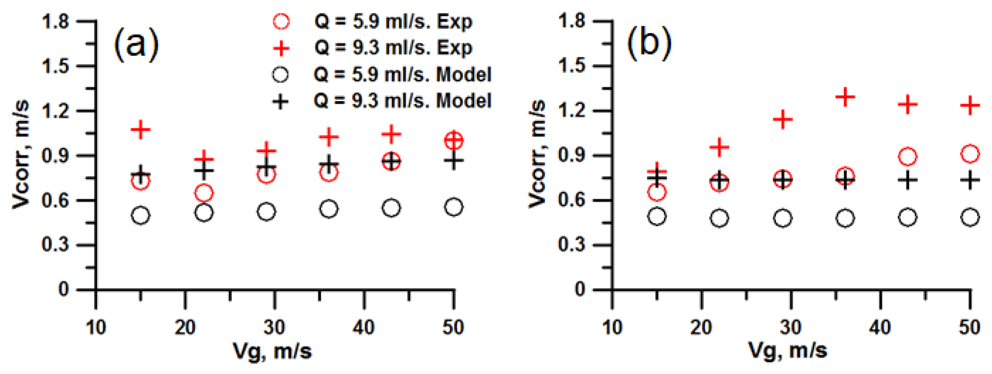
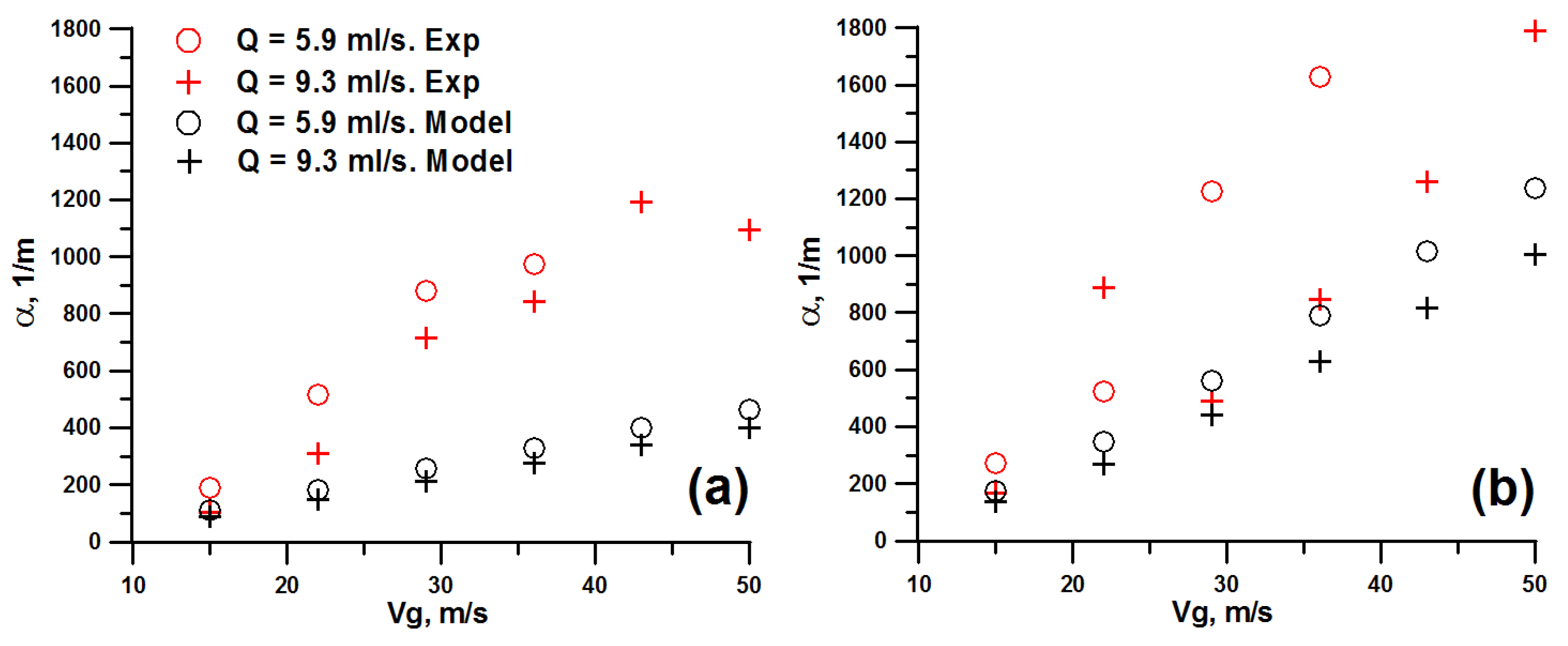
3.3. Modeling and Comparison

The model we used to predict the characteristics of the initial waves is exactly the same as that used in [29]; a very detailed description of the model can be found in that paper. Briefly, the model is based on the Orr–Sommerfeld equation, which is solved in both phases using the divided-attack approach. At the first stage, the liquid is considered rigid and the perturbations in the gas phase induced by a wavy wall are calculated under the assumption of linear response to the perturbations. Then, the tangential and normal stresses at the interface, calculated at the previous stage, are used as boundary conditions for solving the equation in the liquid phase. The solution is sought in the same form as Equation (2), which results in dispersion relationships, α (k) and c(k). An example of a such calculation is shown in Figure 8 for water and WGS2 for the same combination of liquid and gas flow rates. As in [29], we assume that the initial waves are so-called waves of maximum growth, i.e., they evolve from perturbations with a wavenumber corresponding to the position of the maximum of the increment, k_m. Thus, the increment can be calculated as α (k_m), phase velocity— as c(k_m), and frequency as c(k_m) × k_m/2π. An additional complication is that in the model the thickness of an unperturbed film describes the stabilized film flow, which is usually thinner (hence, faster) than the film leaving the slot, where the waves appear. Thus, additional correction for the unperturbed film thickness is required. It is made in accordance with Equation (69) in [29]. Unfortunately, in its present state, the model is not adapted to the case of upward flow. For that reason, the comparison will only be made for downward flow.

The comparison between the model and the experiment is shown in Figure 9, Figure 10 and Figure 11. The comparison is shown for the two liquid flow rates (5.9 and 9.3 mL/s) for the two working liquids (water and WGS2) and the whole range of gas velocities. Qualitatively, the model reproduces the behavior of all three parameters of the waves (frequency, velocity, and increment) with gas velocity, namely, linear growth of f and α with V_G and the weak dependence of c on V_G. The growth of frequency and velocity with the liquid flow rate is reproduced correctly, as well as the increment decrease. The effect of liquid viscosity on modeled increment and velocity is in qualitative agreement with the experiments. However, the effect of viscosity on frequency is not reproduced properly. In the experiments, the frequency barely changes with v in downward flow, but it decreases drastically in the model.

On the quantitative level, the modeled and experimental values are of the same order of magnitude, but the discrepancy is significant. Modeled frequency shows good agreement to the measured one for the lowest liquid flow rate for water; for the larger flow rates, the model overestimates the measurement results (Figure 9a). Based on this observation, it was supposed in [29] that the model works well for low liquid flow rates. However, for different liquid viscosity, the model underestimates the measured frequency for the lowest Q = 5.9 mL/s, whilst a certain agreement is seen for larger Q = 9.3 m/s. Thus, what the model actually overestimates is the importance of liquid flow rate on the frequency of initial waves. The experimental dependence f(Q), such as the one shown in Figure 5d, has a noticeably smaller angle coefficient than the modeled one, and, in contrast to the experiments, there is a viscosity effect. Velocity and increment are underestimated by the model, though for velocity, a better agreement is observed for water, and for increment—for WGS2.

4. Discussion

In the present paper, an experimental and theoretical study of the initial stage of annular gas–liquid flow was conducted as a continuation of work [29]. No systematic experimental studies of the initial waves in annular flow with entrainment were carried out previously. In [27], the closest position of measurements was 15 cm below the inlet. In [31], the measurements were limited by the range of low liquid and gas flow rates. Theoretical stability analysis studies [32,33,34] were aimed at predicting the large-scale waves directly, ignoring the wave formation and development stage. Only in [22] a numerical model was taking the flow development into account.

The present investigation was focused on the effect of flow orientation and the viscosity of a working liquid on the stabilization of the liquid film after it leaves the distributor slot, and on the characteristics of high-frequency fast growing waves, which appear prior to the stabilization of the liquid film. Thus, this paper was aimed at the expansion of the range of applicability of the earlier [29] results.

Upward flow orientation leads to thicker initial film, but also a shorter stabilization length in comparison to downward flow. Both the frequency and increment of the growth of initial waves are lower in the upward flow; the waves’ velocity remains unaffected by flow orientation. In most cases, change in liquid viscosity has a minor effect on film and wave properties, provided that the gas and liquid flow rates are the same. For this reason, the dimensional liquid flow rate (or wetting density if different hydraulic diameters are compared) is a better parameter for the generalization of wave properties than the liquid Reynolds number. The parameter most sensitive to viscosity is the wave increment. The weak effect of viscosity is quite unexpected. One could assume that the actual viscosity of the working liquid decreases at large liquid flow rates or shear rates, but this is not true for the employed liquids and range of shear rates [35].

A possible explanation is that the flow of the liquid film just after leaving the slot is essentially different from the stabilized flow of a gas-sheared liquid film. The momentum of liquid when it is just leaving the slot is induced by the hydrostatic pressure of the liquid in the pressure tank, and not yet affected by the action of gravity or gas shear. Thus, the bulk inertia of the liquid at this stage cannot be immediately compensated by the viscosity, and this is the supposed reason of a weaker viscosity effect than it could be expected for stabilized films. It is possible that for even more viscous liquids, the effect of viscosity would be more prominent and thus detectable.

The modeled characteristics of waves were compared to the measured ones for downward flow with different viscosities. The model reproduces the main qualitative trends in the behavior of wave characteristics, except for the effect of viscosity on wave frequency. On the quantitative level, there is no systematic quantitative agreement between the model and experiment at present.

The reason for this discrepancy is most likely the same as for the weak viscosity effect as described above. The transient character of the flow is also manifested, e.g., in the independence of film thickness in the area of interest on liquid and even gas (for downward case) flow rate or the independence of wave velocity on gas velocity and flow orientation. It could be expected that the velocity profile inside the liquid film changes essentially between the slot outlet and the point of stabilization of film thickness and that these changes affect the wave generation.

Further development of the model should be aimed at taking this aspect of the downstream evolution of the flow into account. In addition, the simplified analysis of the wave structure according to Equation (2) could be improved towards multi-modal or non-modal analysis, which would require more advanced experimental and theoretical approaches.

References

1. Webb, D.R.; Hewitt, G.F. Downwards co-current annular flow. Int. J. Multiph. Flow 1975, 2, 35–49. [Google Scholar] [CrossRef]
2. Azzopardi, B.J. Disturbance wave frequencies, velocities and spacing in vertical annular two-phase flow. Nucl. Eng. Des. 1986, 92, 121–133. [Google Scholar] [CrossRef]
3. Han, H.; Zhu, Z.; Gabriel, K. A study on the effect of gas flow rate on the wave characteristics in two-phase gas–liquid annular flow. Nucl. Eng. Des. 2006, 236, 2580–2588. [Google Scholar] [CrossRef]
4. Farias, P.S.C.; Martins, F.J.W.A.; Sampaio, L.E.B.; Serfaty, R.; Azevedo, L.F.A. Liquid film characterization in horizontal, annular, two-phase, gas–liquid flow using time-resolved laser-induced fluorescence. Exp. Fluids 2012, 52, 633–645. [Google Scholar] [CrossRef]
5. Shedd, T.A.; Newell, T.A. Characteristics of the liquid film and pressure drop in horizontal, annular, two-phase flow through round, square and triangular tubes. J. Fluids Eng. 2004, 126, 807–817. [Google Scholar] [CrossRef]
6. Schubring, D.; Shedd, T.A. Wave behavior in horizontal annular air–water flow. Int. J. Multiph. Flow 2008, 34, 636–646. [Google Scholar] [CrossRef]
7. Kaji, R.; Azzopardi, B.J. The effect of pipe diameter on the structure of gas/liquid flow in vertical pipes. Int. J. Multiph. Flow 2010, 36, 303–313. [Google Scholar] [CrossRef]
8. Alamu, M.B.; Azzopardi, B.J. Wave and drop periodicity in transient annular flow. Nucl. Eng. Des. 2011, 241, 5079–5092. [Google Scholar] [CrossRef]
9. Vasques, J.; Cherdantsev, A.; Cherdantsev, M.; Isaenkov, S.; Hann, D. Comparison of disturbance wave parameters with flow orientation in vertical annular gas-liquid flows in a small pipe. Exp. Therm. Fluid Sci. 2018, 97, 484–501. [Google Scholar] [CrossRef]
10. Mori, K.; Kondo, Y.; Kaji, M.; Yagishita, T. Effects of Liquid Viscosity on Characteristics of Waves in Gas-Liquid Two-Phase Flow: Characteristics of Huge Waves and Disturbance Waves. JSME Int. J. Ser. B 1999, 42, 658–666. [Google Scholar] [CrossRef] [Green Version]
11. Clark, W.W.; Campbell, G.B.; Hills, J.H.; Azzopardi, B.J. Viscous effects on the interfacial structure of falling liquid film/co-current gas systems. In Proceedings of the 4th International Conference on Multiphase Flow, New Orleans, LA, USA, 27 May–1 June 2001. [Google Scholar]
12. Bousman, W.S. Studies of two-Phase Gas-Liquid Flow in Microgravity. Ph.D. Thesis, University of Houston, Houston, TX, USA, 1994. [Google Scholar]
13. Mantilla, I. Mechanistic Modeling of Liquid Entrainment in Gas in Horizontal Pipes. Ph.D. Thesis, University of Tulsa, Tulsa, OK, USA, 2008. [Google Scholar]
14. Setyawan, A.; Indarto; Deendarlianto. The effect of the fluid properties on the wave velocity and wave frequency of gas–liquid annular two-phase flow in a horizontal pipe. Exp. Therm. Fluid Sci. 2016, 71, 25–41. [Google Scholar] [CrossRef]
15. Sekoguchi, K.; Nakazatomi, M.; Takeishi, M.; Shimizu, H.; Mori, K.; Miyake, G. Pressure Effect on Velocity of Liquid Lumps in Vertical Upward Gas-Liquid Two-Phase Flow. JSME Int. J. Ser. 2 1992, 35, 380–387. [Google Scholar] [CrossRef] [Green Version]
16. Sawant, P.; Ishii, M.; Hazuku, T.; Takamasa, T.; Mori, M. Properties of disturbance waves in vertical annular two-phase flow. Nucl. Eng. Des. 2008, 238, 3528–3541. [Google Scholar] [CrossRef]
17. Wang, C.; Zhao, N.; Feng, Y.; Sun, H.; Fang, L. Interfacial wave velocity of vertical gas-liquid annular flow at different system pressures. Exp. Therm. Fluid Sci. 2018, 92, 20–32. [Google Scholar] [CrossRef]
18. Berna, C.; Escrivá, A.; Muñoz-Cobo, J.L.; Herranz, L.E. Review of droplet entrainment in annular flow: Interfacial waves and onset of entrainment. Prog. Nucl. Energy 2014, 74, 14–43. [Google Scholar] [CrossRef]
19. Dasgupta, A.; Chandraker, D.K.; Kshirasagar, S.; Reddy, B.R.; Rajalakshmi, R.; Nayak, A.K.; Hewitt, G.F. Experimental investigation on dominant waves in upward air-water two-phase flow in churn and annular regime. Exp. Therm. Fluid Sci. 2017, 81, 147–163. [Google Scholar] [CrossRef]
20. Cuadros, J.L.; Rivera, Y.; Berna, C.; Escrivá, A.; Muñoz-Cobo, J.L.; Monrós-Andreu, G.; Chiva, S. Characterization of the gas-liquid interfacial waves in vertical upward co-current annular flows. Nucl. Eng. Des. 2019, 346, 112–130. [Google Scholar] [CrossRef]
21. Lin, R.; Wang, K.; Liu, L.; Zhang, Y.; Dong, S. Application of the image analysis on the investigation of disturbance waves in vertical upward annular two-phase flow. Exp. Therm. Fluid Sci. 2020, 114, 110062. [Google Scholar] [CrossRef]
22. Fan, W.; Li, H.; Anglart, H. Numerical investigation of spatial and temporal structure of annular flow with disturbance waves. Int. J. Multiph. Flow 2019, 110, 256–272. [Google Scholar] [CrossRef]
23. Han, H.; Gabriel, K. A numerical study of entrainment mechanism in axisymmetric annular gas-liquid flow. J. Fluids Eng. 2007, 129, 293–301. [Google Scholar] [CrossRef]
24. Yang, J.; Narayanan, C.; Lakehal, D. Large Eddy & Interface Simulation (LEIS) of disturbance waves and heat transfer in annular flows. Nucl. Eng. Des. 2017, 321, 190–198. [Google Scholar]
25. Alekseenko, S.V.; Cherdantsev, A.V.; Cherdantsev, M.V.; Isaenkov, S.V.; Markovich, D.M. Study of formation and development of disturbance waves in annular gas–liquid flow. Int. J. Multiph. Flow 2015, 77, 65–75. [Google Scholar] [CrossRef]
26. Hall Taylor, N.; Nedderman, R.M. The coalescence of disturbance waves in annular two phase flow. Chem. Eng. Sci. 1968, 23, 551–564. [Google Scholar] [CrossRef]
27. Zhao, Y.; Markides, C.N.; Matar, O.K.; Hewitt, G.F. Disturbance wave development in two-phase gas–liquid upwards vertical annular flow. Int. J. Multiph. Flow 2013, 55, 111–129. [Google Scholar] [CrossRef] [Green Version]
28. Wolf, A.; Jayanti, S.; Hewitt, G.F. Flow development in vertical annular flow. Chem. Eng. Sci. 2001, 56, 3221–3235. [Google Scholar] [CrossRef]
29. Isaenkov, S.V.; Cherdantsev, A.V.; Vozhakov, I.S.; Cherdantsev, M.V.; Arkhipov, D.G.; Markovich, D.M. Study of primary instability of thick liquid films under strong gas shear. Int. J. Multiph. Flow 2019, 111, 62–81. [Google Scholar] [CrossRef]
30. Pan, L.-M.; He, H.; Ju, P.; Hibiki, T.; Ishii, M. Experimental study and modeling of disturbance wave height of vertical annular flow. Int. J. Heat Mass Transfer. 2015, 89, 165–175. [Google Scholar] [CrossRef]
31. Alekseenko, S.V.; Aktershev, S.P.; Cherdantsev, A.V.; Kharlamov, S.M.; Markovich, D.M. Primary instabilities of liquid film flow sheared by turbulent gas stream. Int. J. Multiph. Flow 2009, 35, 617–627. [Google Scholar] [CrossRef]
32. Andreussi, P.; Asali, J.C.; Hanratty, T.J. Initiation of roll waves in gas-liquid flows. AIChE J. 1985, 31, 119–126. [Google Scholar] [CrossRef]
33. Hewitt, G.F.; Hall-Taylor, N.S. Annular Two-Phase Flow; Pergamon Press: Oxford, UK, 1970. [Google Scholar]
34. Asali, J.C.; Hanratty, T.J. Ripples generated on a liquid film at high gas velocities. Int. J. Multiph. Flow 1993, 19, 229–243. [Google Scholar] [CrossRef]
35. Dontula, P.; Macosko, C.W.; Scriven, L.E. Does the viscosity of glycerin fall at high shear rates? Ind. Eng. Chem. Res. 1999, 38, 1729–1735. [Google Scholar] [CrossRef]
Figure 1. (a) Scheme of the inlet and layout of the camera and the illumination lamp for the shadow method; (b) instantaneous image of the film profile on one wall of the pipe and a fragment of a spatiotemporal matrix of film thickness.
Applsci 10 04366 g001
Figure 2. Dependence of the time-averaged film thickness on the downstream coordinate: (a) water–glycerol solution (WGS1), QL = 10.3 mL/s, VG = 22 m/s; (b) WGS1, QL = 10.3 mL/s, VG = 43 m/s.
Applsci 10 04366 g002
Figure 3. Maximum film thickness near the inlet versus gas velocity: (a) Water; (b) WGS2.
Applsci 10 04366 g003
Figure 4. Length of the stabilization zone. (a,b) The effect of liquid viscosity at a fixed liquid flow rate for downward (a) and upward (b) flows. (c) The effect of flow orientation. (d) The effect of the liquid flow rate for a fixed gas velocity, VG = 29 m/s.
Applsci 10 04366 g004
Figure 5. Frequency of the initial waves. (a,b) The effect of liquid viscosity at a fixed liquid flow rate for downward (a) and upward (b) flows. (c) The effect of flow orientation. (d) The effect of the liquid flow rate for a fixed gas velocity, VG = 29 m/s.
Applsci 10 04366 g005aApplsci 10 04366 g005b
Figure 6. Phase velocity of the initial waves. (a,b) The effect of liquid viscosity at a fixed liquid flow rate for downward (a) and upward (b) flows. (c) The effect of flow orientation. (d) The effect of a liquid flow rate for a fixed gas velocity, VG = 29 m/s.
Applsci 10 04366 g006
Figure 7. Increment of the amplitude growth of the initial waves. (a,b) The effect of liquid viscosity at a fixed liquid flow rate for the downward (a) and upward (b) flows. (c) The effect of flow orientation. (d) The effect of the liquid flow rate for a fixed gas velocity, VG = 29 m/s.
Applsci 10 04366 g007
Figure 8. Calculated dispersion relationships. (a) Spatial increment of the amplitude growth; (b) Phase velocity of the waves. Q = 5.9 mL/s; VG = 22 m/s, downward flow.
Applsci 10 04366 g008
Figure 9. Comparison of the measured against the calculated wave frequency: (a) water; and (b) WGS2.
Applsci 10 04366 g009
Figure 10. Comparison of the measured against the calculated wave velocity: (a) water; and (b) WGS2.
Applsci 10 04366 g010
Figure 11. Comparison of the measured against the calculated increment of amplitude growth: (a) water; and (b) WGS2.
Applsci 10 04366 g011