The case study in this research is related to a micro-company that has a collection center for regional products associated with the cold and dry food chain, which must be packaged according to demand and distributed to customers located on different routes. The objective of this work is to minimize costs and delivery time. The company requires the monitoring of the logistics performance indicators; the following steps were followed for the solution, which could be generalized for different organizations intending to reduce logistics and transportation costs.
4.1. Analysis of the Distribution Process
In order to better understand the context of the studied company, different mapping techniques were carried out with information collected from interviews and guided visits within the company by the director with the aim of improving our understanding of its operation.
The work team met with the company director and staff from the distribution process. The director shared information and showed the complete supply chain processes and the available information required to develop the solution through a guided visit.
On the other hand, the administrator of the regional products (dry and cold distribution process) gave a mapping tour of all the delivery routes; the maps for each route were constructed and data were collected and validated. The solution was presented to the director and distributors to validate the graphical interface.
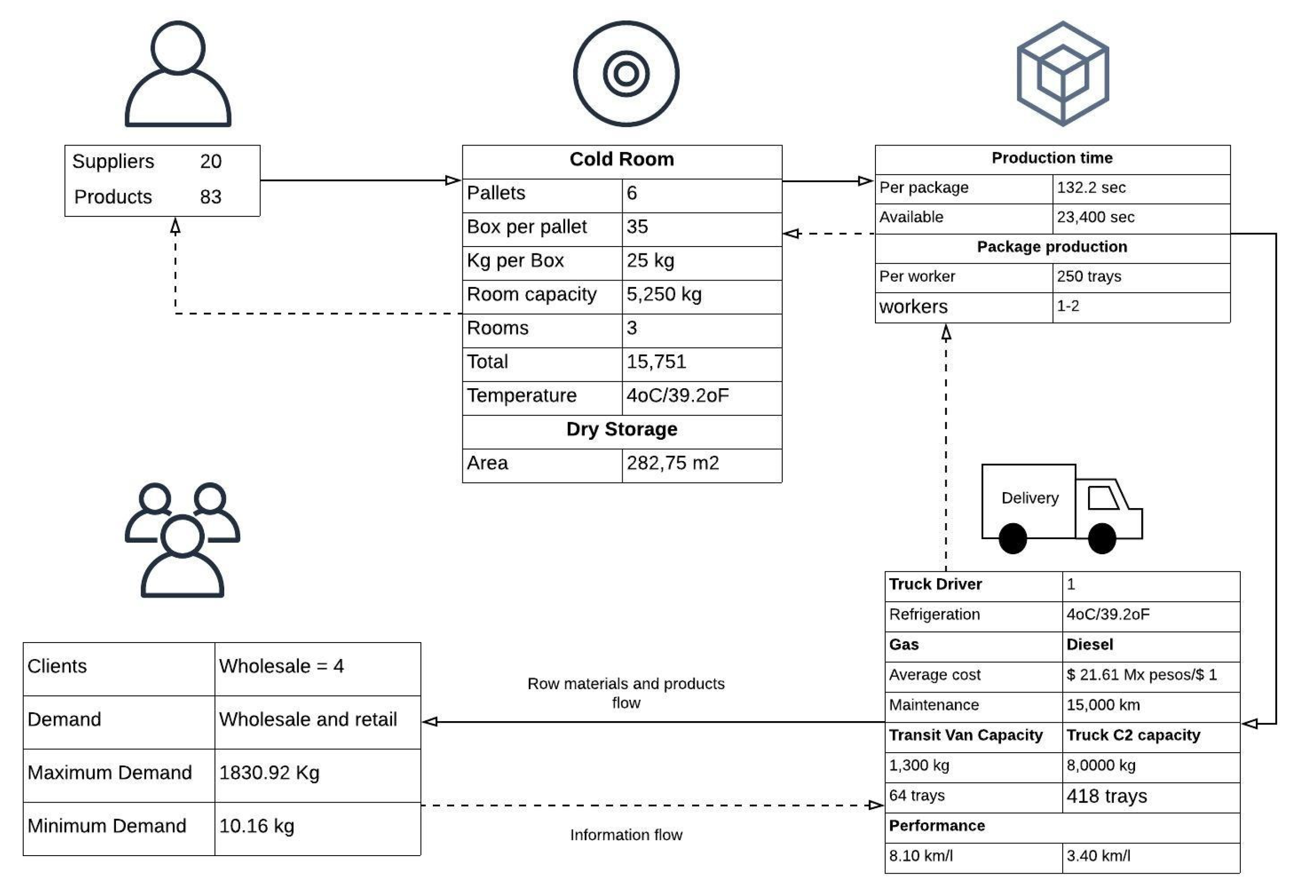
A supply chain map was made with the most important aspects of the company’s current supply chain. As already mentioned, the first contact with the company was made through interviews and a guided visit, which provided more clarity on the vision of how the organization operates, as shown in
Figure 1.
4.4. Causal Loop Diagram Creation
For the variables analyzed in the previous step, a causal diagram related to variable behavior and interaction was created for the company’s distribution process, as shown in
Figure 2.
The causal loop diagram shows the variables that are interrelated at the moment of instigating the wholesale and retail demand distribution process. The influence of the interaction among variables is depicted by the symbols positive (+)—defining a reinforcement variable—and negative (−)—defining a balancing variable. The diagram has five feedback loops that are responsible for balancing the system (B1, B2 is B1-2, B3, B4, and B5). Each loop is explained according to its relationship and conditions; B refers to the balancing loop.
The first causal loop is B1-B2 is B1-2, which shows the relationship among warehouse products, demand, distribution, product delivery, routes, costs, profit, investments, number of trucks, distribution capacity and clients; the B1 loop closes with wholesale demand, and at the same time, B2 closes the loop with retail demand. B3 is the relationship between warehouse products and distribution process, and B4 is the relationship between warehouse products and production package. Finally, B5 is the relationship between delivery routes and costs.
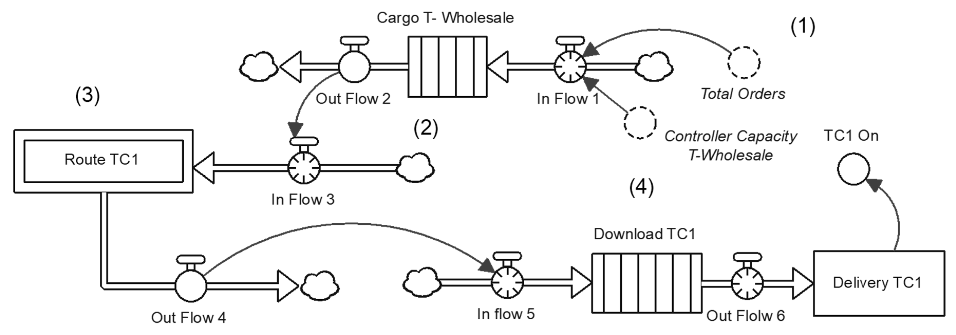
4.5. Current Model Simulation
Based on the variables determined for the model and causal diagram, the dynamics simulation model was formulated by using Stella® Architect software. The model was structured based on the mathematical equations used to calculate the different variable values. The considerations taken into account for the designed model were as follows: wholesale demand (kg) when less or equal to 1300 kg; that is, demand less than or equal to the capacity in kilograms of the Ford Transit vehicle. The demand for wholesale is up to 8000 kg; that is, the C2 truck capacity is considered in kilograms.
Under these considerations, a package needed to be specified as a container with the following measurements: 0.60 m (length), 0.32 m (width) and 0.40 cm (height). The different products are then placed inside and delivered to the customers. Due to the dimensions of the container, the space within the transportation vehicle units is restricted: the possible volume to be transported is 0.0768 m3.
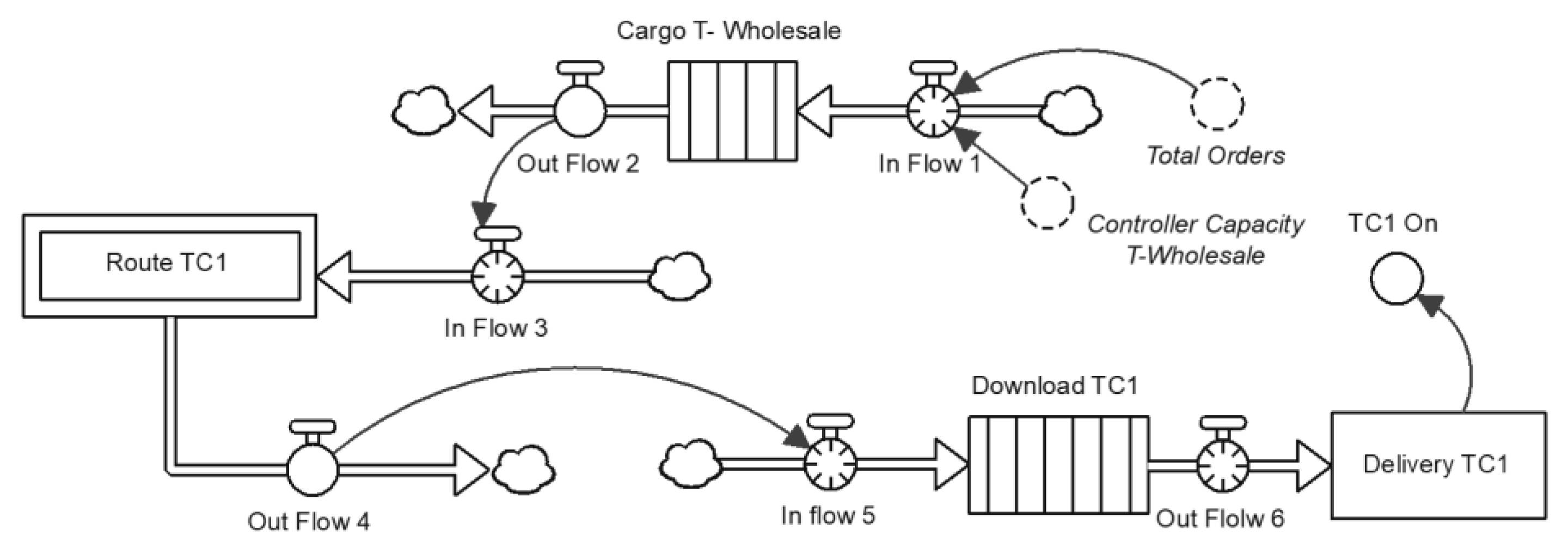
The base model is structured in a logical way, representing the real structure of the system under study (the distribution process), consisting of loading activities, transporting the product to customers, unloading and delivering the product to customers.
Figure 3 shows the varying wholesale demand using the Ford Transit vehicle.
In the model for the current scenario, a single load, route and unloading is considered, and the products are delivered to only one customer. The model considers delivery to several customers on the same route: it may carry out distribution to one, two or three customers. Product loading is performed only once when all the goods to be delivered to all the customers are loaded. Moreover, the distance traveled in the routes to reach each location is considered, as well as the unloading maneuvers that are conducted individually.
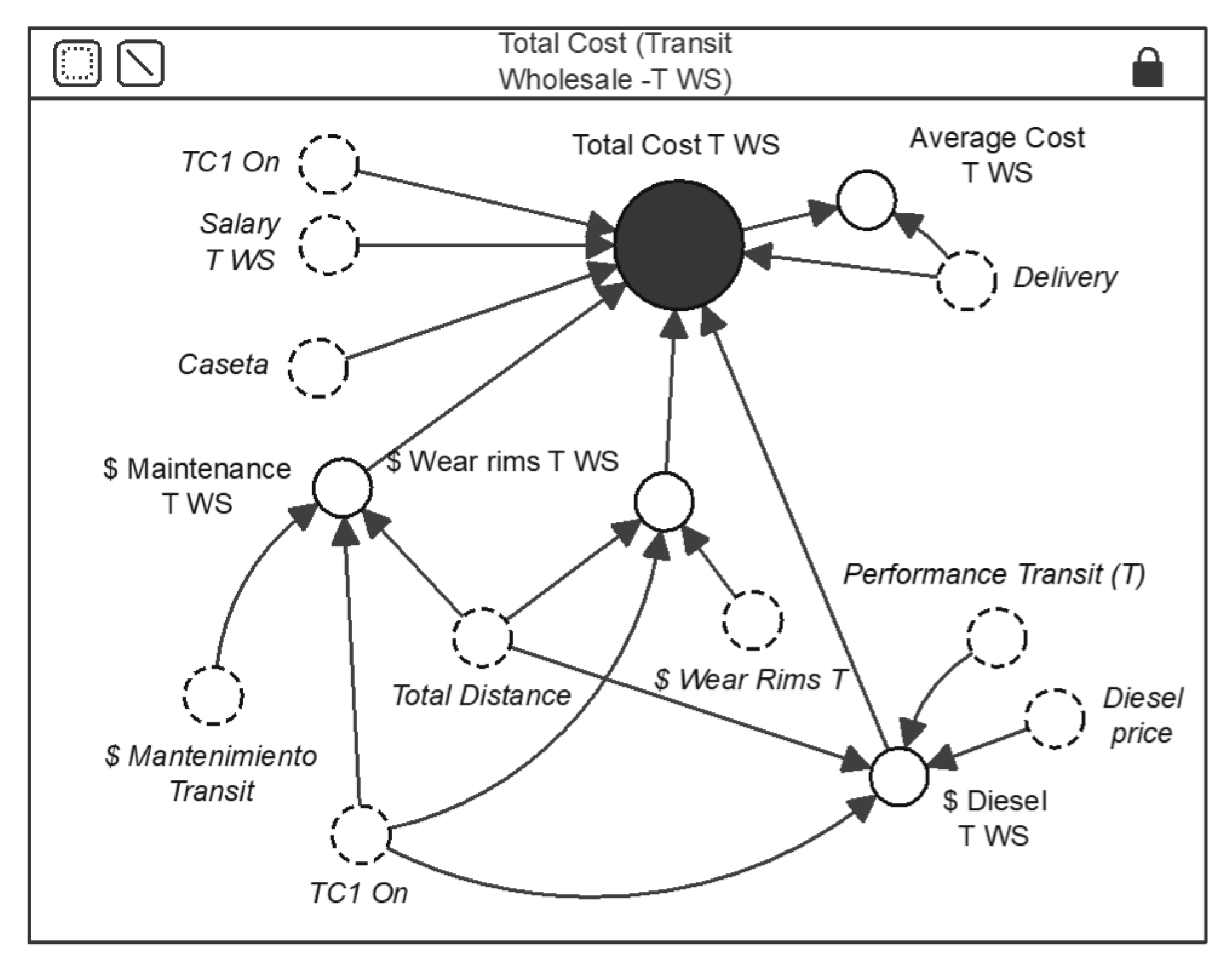
Figure 4 shows the inherent wholesale delivery costs.
The costs considered in goods distribution, including the truck driver’s salary, vehicle maintenance, tire wearing, diesel consumption and tolls in a given case, are all considered. These costs are added to obtain the total distribution cost. The proposed model is based on variables and parameters, for which different equations were required. The determination of the type of variables was also necessary according to the symbols suggested in [
11]; that is, level, auxiliary, flow or parameter variables. Below is a summary of the variables based on their category:
Level:
where
WiTl = wholesale items, total load;
WmIf = wholesale meat, input flow;
WmOf = wholesale meat, output flow.
where
R1
LT = Route 1, load transport;
R1
WmIf = Route 1, wholesale meat input flow;
R2
WmOf = Route 2, wholesale meat output flow.
where
R1
LTd = Route 1, load, transport deliveries;
R1
WmfdOf = Route 1, wholesale meat, final delivery output flow.
Auxiliary:
where
Tt = transit time;
Ltpe = loading time per employee;
D = demand.
where
Ct = cooking time (time during which wholesale products remain in the Transit vehicle);
C1
d =
C1 distance;
TVs = Transit vehicle speed.
where
WmC = wholesale maintenance cost;
TwC = tire wearing cost;
DC = diesel cost;
S = salary;
TbC = toll cost;
LDgt = loading time;
Dl = deliveries;
TTnt = Transit truck number of trips.
Flow Variables:
where
MMIF = wholesale meat input flow.
4.6. Current Model Validation
In this section, model validation was performed by means of four tests: (1) proper limits, (2) structure verification, (3) dimensional consistency and (4) extreme condition.
According to [
36], the first test should consider if the current model meets the purpose for which it was created. In this case study, the main objectives determined were cost reduction and distribution time. The proposed model considered cost indicators (vehicle maintenance, tire wearing, tolls, salary and diesel), as well as time (route and hours worked to complete delivery). The second test verified the model structure. In this test, the current system structure must be compared with the existing model, as shown in
Figure 5.
The dimensional consistency test, according to [
36], seeks to assess and analyze every mathematical equation and model parameter. Stella
® Architect, provides a tool to conduct the vehicle unit tests. A revision of the model vehicle units was performed considering 251 equations and 410 variables, finding 100% consistency. Finally, the extreme condition test was carried out with the aim of determining whether the model operated logically when the parameter values drastically changed. The change made to this test was the lack of demand; by eliminating the demand, the model should not reflect any behavior, since it is the demand that “pulls” the entire system—that is, the values must be zero. As both wholesale and retail demand were modified to 0 (zero), the model behaved as expected; i.e., no movement indication was observed in the flows. Thus, the structural tests conducted validated the developed model.
4.7. Quantitative Scenarios Based on Key Performance Indicator Construction
In this part of the method, different quantitative scenarios were simulated in the model; thus, a sensitivity analysis was performed to determine which variables were more sensitive to different parameters.
Three scenarios were considered; the first one represented a less favorable situation for the organization, the second one represented the normal distribution process conditions and the third one represented a favorable situation for the organization. The following data (
Table 4) show the normal scenario as an example of how the parameters were defined.
To define indicators, the data in
Table 4 were considered to generate the total result shown in
Table 5. To explain this idea, two types of equations must be created: one summative (profit, distribution cost) and the other average (vehicle usage capacity, transportation cost/Kg, and cost–profit ratio).
According to the information in
Table 4, the variable total profit (
$) shown in
Table 5 is the result from each profit according to the transit vehicle and C2 truck generated with the following formula
where
TP (
$) = total profit;
Ti = Transit vehicle;
i = routes—Ciudad Obregón, Etchojoa, Bácum, and Campo 5. The final parameter for
TP (
$) was 73,627.4 + 32,741.3 + 21,180.5 + 3994.8 = 131,544.
The average vehicle usage capacity (AUVC) is defined by Equation (9):
where
AUVC = average vehicle usage capacity;
ATi = average of each Transit vehicle;
i = routes—Ciudad Obregón, Etchojoa, Bácum, and Campo 5.
The average vehicle usage capacity parameter in
Table 5 was obtained according to an AUVC of (39.06 + 56.25 + 34.38 + 39.06)/4 = 41.21.
The seven key performance indicators selected to investigate these scenarios were considered with two requirements: (1) the indicator showed its impact on the results obtained, and (2) the organization had not considered the indicator within their analysis. Thus, the selected indicators were as follows: (1) wholesale demand, which is measured in kilograms ordered by each customer; (2) retail demand, which refers to the number of packages ordered by one or several customers; (3) diesel price, expressed in Mexican pesos per liter; (4) net income per kilogram, which considers the income per kilogram; (5) net income per package, representing the income obtained per package; (6) cost per tire, which refers to tire purchase cost; and (7) maintenance cost, considering servicing charges for the distribution vehicle units.
Table 6 shows a summary of the wholesale distribution including the six relevant variables.
The three wholesale product distribution scenarios showed that the optimistic scenario considerably increased the total profit, mainly due to the consideration of a greater number of customers (i.e, six potential customers).
When considering weekly and average demands for each of the customers, the option of purchasing another Transit vehicle was not considered necessary because, taking into account the operating hours per month (224 h; i.e., 8 h a day for four weeks), the vehicle was only used for 58 h.
The number of hours used by the vehicle increased significantly in the optimistic scenario compared with the normal one, with a difference of 78.76 h compared to that of the Transit vehicle and 65.72 h considering the C2 truck. Lastly, cost-related information regarding the three scenarios is described in
Table 6.
The purchase of diesel represented the highest cost in the three simulated scenarios, which indicated the need to pay greater attention to the distance traveled by the vehicles and their fuel yield since this will determine on average 56.49% of the total distribution cost. In addition, one of the findings referred to vehicle unit maintenance and tire wearing costs, which contributed 9.21% and 3.66% of the total costs, respectively.
4.8. Graphical User Interface Development
Lastly, and to continue the project’s congruency, a graphic interface was created to support decision-making (
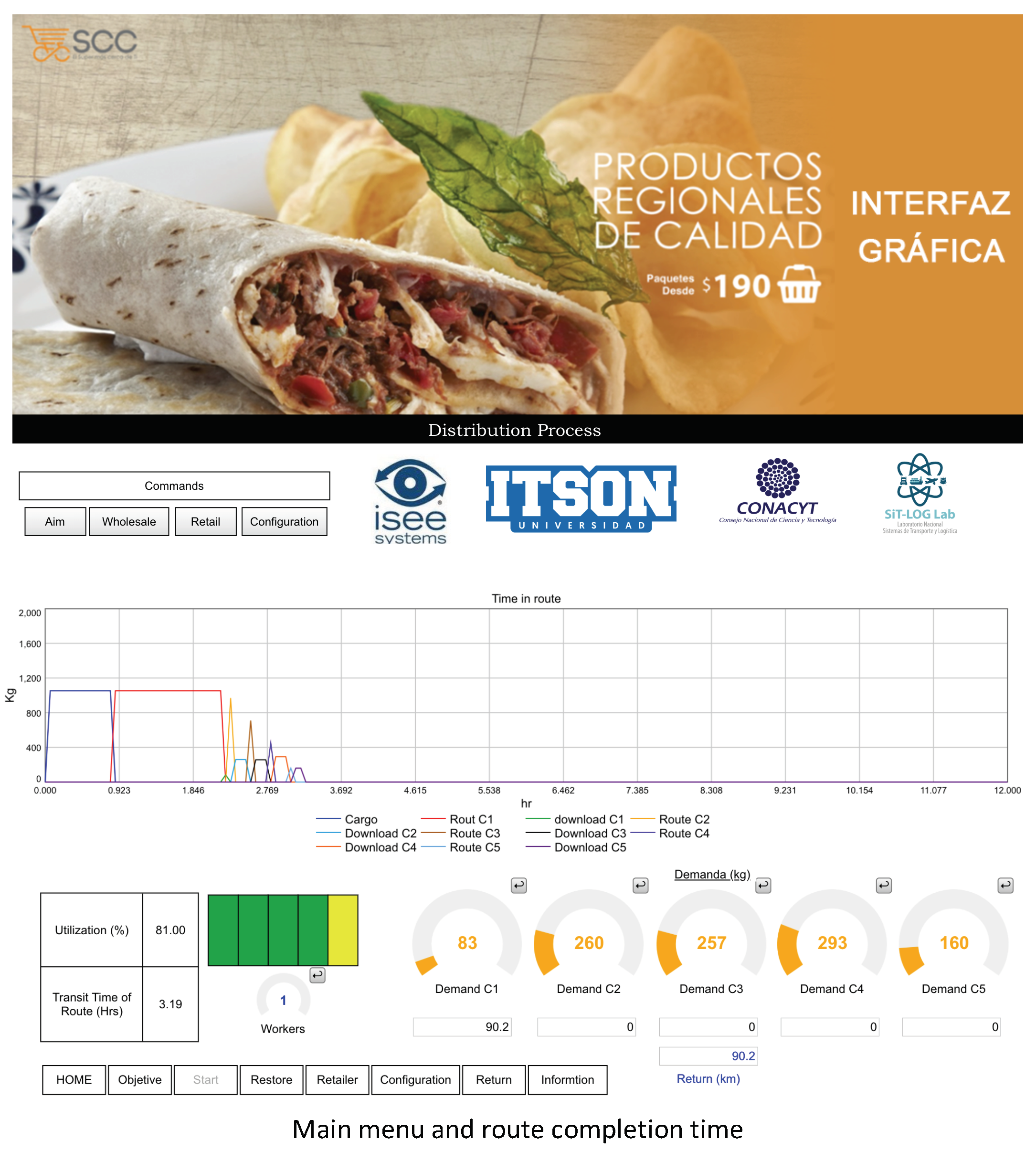
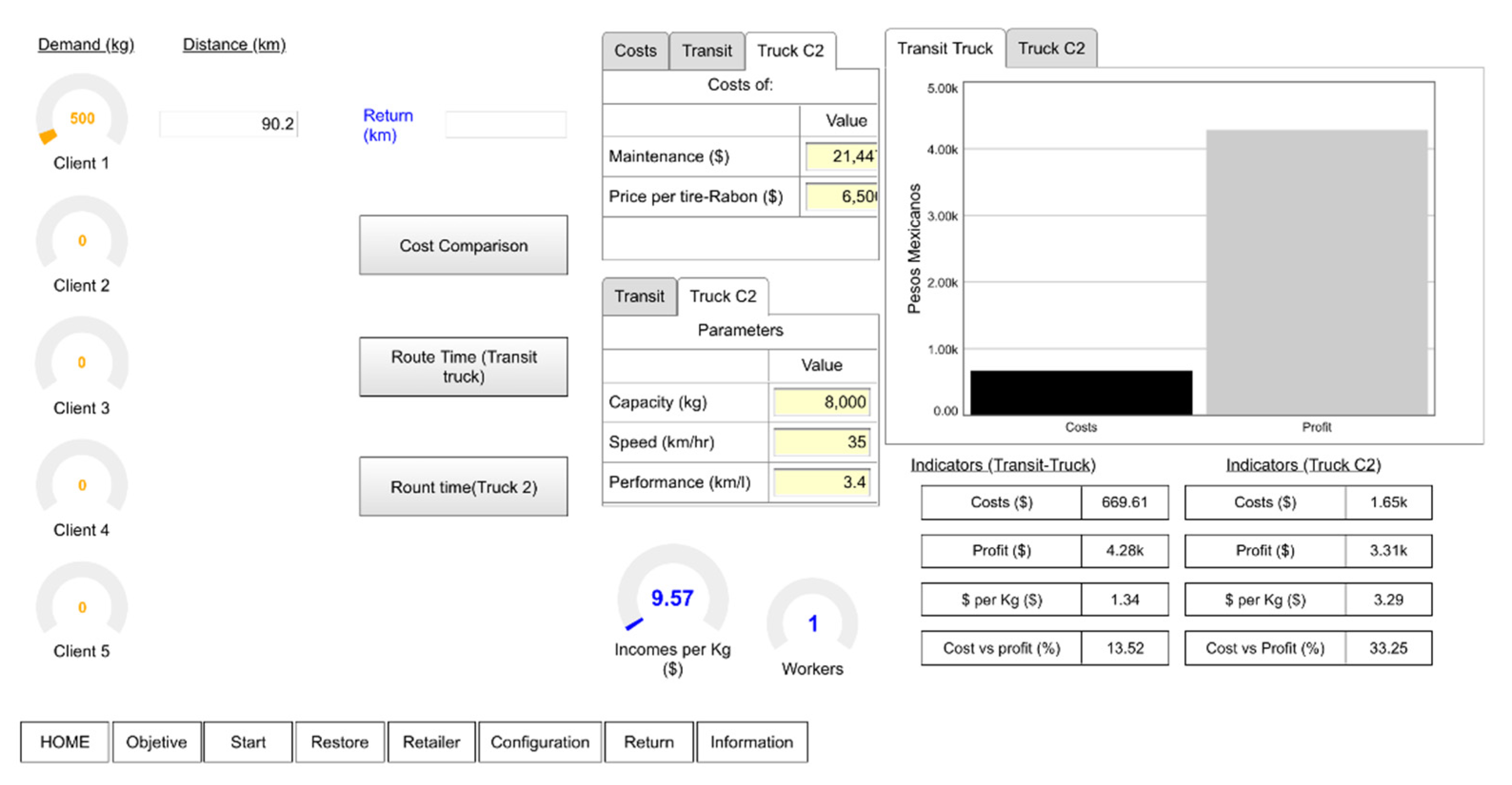
Figure 6). The interface was divided into three main parts on screens that provide information (i.e., Home, Settings and Objective). The screens analyzed wholesale demand (for 1 to 5 customers, Transit and C2 Truck, “n” customers, route completion time and cost comparison), and the screens focused on analyzing retail demand (for 1 to 5 customers, Transit vehicle and C2 Truck, “n” customers, route completion time and cost comparison).
The objective of the first screen is to give the interface a professional look and link the organization under study with its sponsors. Navigation buttons are placed on the interface screens and buttons that provided information with regards to the screen are shown, where one serves as a “tutorial” and indicates the functioning of the rest of the buttons. After the home screen, the functional interface appears, as shown in
Figure 7.
This screen is related to the wholesale demand key performance indicators, with a focus on analyzing the demand of 1–5 customers individually; an information button indicates the correct way to use the screen. Within this modality, customer demand and distances must be entered individually. There are also two setting tables in which the main model parameters operate and carry out significant analysis. It is also necessary to show the indicators related to delivery times and vehicle capacity usage;
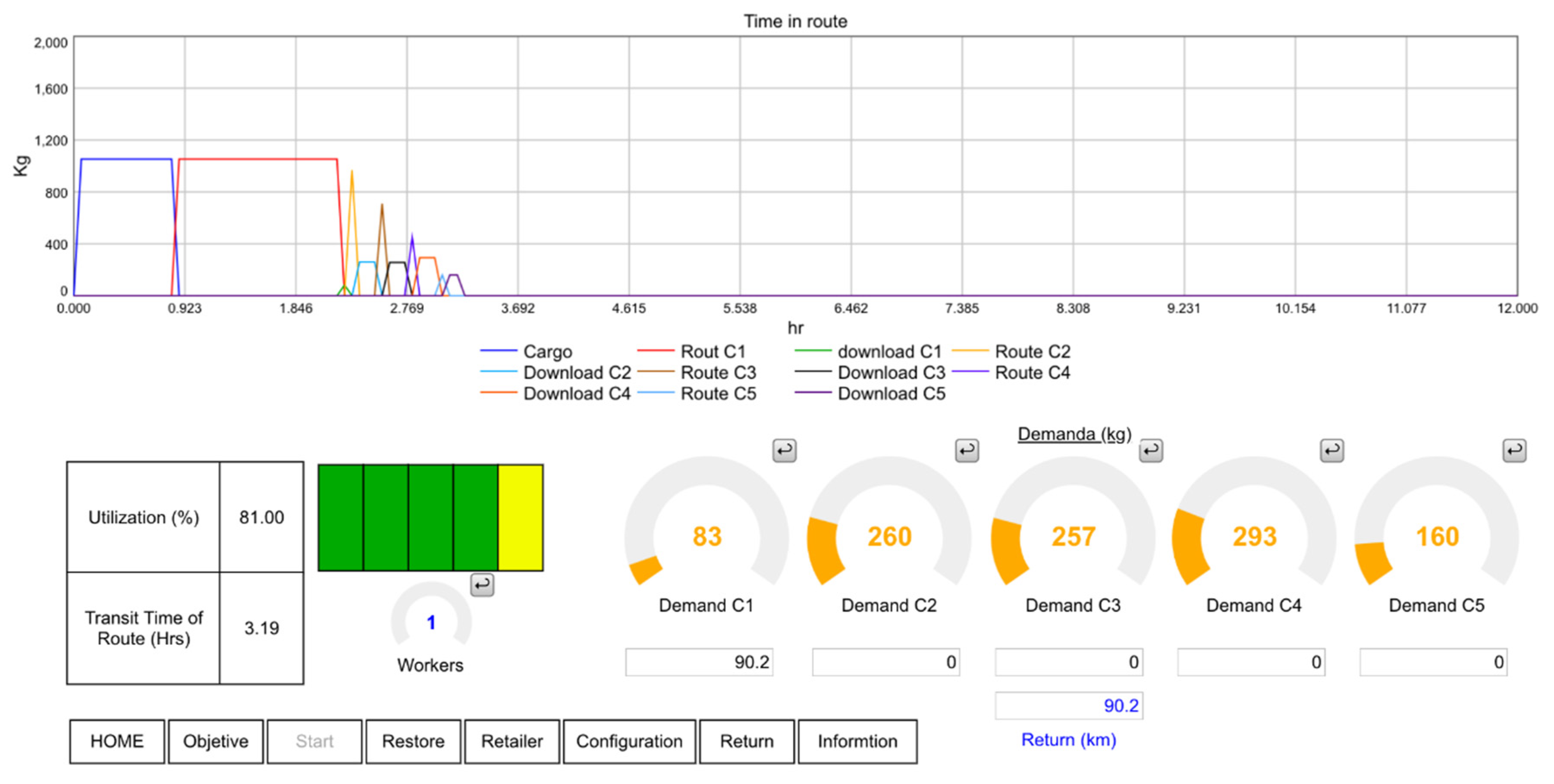
Figure 8 shows the screen designed for this purpose.
The time analysis screen related to the delivery route may be observed; as with the other screens, by modifying the customer demands or distances, the graph shown in the upper part is directly affected. Within this screen, the route completion time indicators are found, estimating vehicle usage percentage in hours, shown as numerical data and in an animation that changes color depending on the vehicle unit usage level, varying from red (empty) and yellow (loaded) to green (full).
On this screen, the route completion time indicators are found, which estimate the vehicle usage percentage in hours, shown as numerical data and in an animation that changes color depending on the vehicle unit usage level, varying from red (empty) and yellow (loaded), to green (full).

 ,
, 


