Abstract
Heart diseases are in the front rank among several kinds of life threats, due to its high incidence and mortality. Regarded as a powerful tool in the diagnosis of the cardiac disorder and arrhythmia detection, analysis of electrocardiogram (ECG) signals has become the focus of numerous researches. In this study, a feature extraction method based on the bispectrum and 2D graph Fourier transform (GFT) was developed. High-order matrix founded on bispectrum are extended into structured datasets and transformed into the eigenvalue spectrum domain by GFT, so that features can be extracted from statistical quantities of eigenvalues. Spectral features have been computed to construct the feature vector. Support vector machine based on the radial basis function kernel (SVM-RBF) was used to classify different arrhythmia heartbeats downloaded from the Massachusetts Institute of Technology - Beth Israel Hospital (MIT-BIH) Arrhythmia Database, according to the Association for the Advancement of Medical Instrumentation (AAMI) standard. Based on the cross-validation method, the experimental results depicted that our proposed model, the combination of bispectrum and 2D-GFT, achieved a high classification accuracy of 96.2%.
1. Introduction
According to the World Health Organization (WHO), about one third of the world’s deaths are caused by cardiovascular disease every year statistically [1]. Cardiovascular disease has become one of the leading causes of death from non-infectious and non-transmissible diseases in the world [2]. Therefore, prevention and early diagnosis are key for a successful clinical management.
Arrhythmia is an important group of diseases in cardiovascular disease. The diagnosis of arrhythmia mainly depends on the electrocardiogram (ECG). ECG is an important modern medical tool that can record the process of cardiac excitability, transmission, and recovery. It reflect the degree of myocardial cell damage, development process, functional structure of atrium and ventricle [3]. Detection of irregular heartbeats from ECG signals is a significant task for the automatic diagnosis of cardiovascular disease.
The extraction of features from the ECG signal is a key step for ECG recognition, as it allows to greatly enhance and extract the characteristics of the signal. The quality of morphological features extraction in the ECG greatly affects the recognition and classification rate of ECG signals. Generally, the features in the time domain include the amplitude, the RR interval, the duration, and the shape of the clinical components (P-wave, QRS-complex, and T-wave) of ECG [4,5,6]. The features in the transform domain embody different diagnostic features extracted by different signal processing techniques, such as the autoregressive model coefficients, principal component analysis, and geometric attributes based on an image [7,8,9,10]. Those features can be fed into conventional machine learning models, for instance, decision trees, support vector machine, k nearest neighbor, and Bayesian algorithm [11,12,13,14] to realize heartbeats classification.
The high-order spectra (HOS) has been widely used in the analysis of bio-medical signals [15,16]. The high order statistics method is insensitive to Gaussian noise, thus, becoming a suitable method for feature extraction. Bispectrum is the simplest high order spectra, sharing the characteristics of time shift invariance, phase retention and scale variability. Bispectrum and histogram have been used in the analysis of ECG signals [10,17,18]. A method for the automated identification of Coronary Artery Disease was proposed in [10], which achieved 98.99% accuracy with 31 cumulants features. Zhelin, Y. et.al [17] proposed an Atrial Fibrillation (AF) identification system based on 57 features including bispectrum and histogram. They got an accuracy of 98.72%. A combination of both vertical and horizontal histogram and pattern based heuristic methods were used in [18] for the detection of P, Q, R, S and T waves. The detection accuracy for P and T wave were 92.2% and 96.7%, respectively.
Over the past decade, the graph signal processing (GSP) based on spectral graph theory [19] has been proven to be a real promising method in many application areas [20,21,22]. Analogous to the Fourier transform (FT), GFT, as the foundation of GSP, is a data conversion method [23]. GSP visualizes spatiotemporal data as a 2D graph signal, Chindanur N. B. et al. developed a 3D-GFT model that renders better than its 2D counterpart [24].
This study intends to develop a new method which combines the insensitivity of the bispectrum and the merits of GFT. Features fed into the classifier are spectral flatness, spectral brightness and spectral roll-off [25]. To assess the performance of the proposed method and compare it with previous algorithms, confusion matrix, accuracy (), error rate (), Macro-averaged F-score (), sensitivity (), specificity (), and positive predictive rate () are used to analyze quantitatively. The analysis results of experimental signals based on the widely recognized MIT-BIH Arrhythmia Database [26] indicated that the proposed method can effectively differentiate several beat types.
The article is structured as follows: System model is displayed in Section 2, which includes the fundamental steps, principles and definition needed. Section 3 lists the dataset and the evaluation index. The details and reports of the experiments are presented in Section 4. Conclusion and future direction are drawn in Section 5.
2. Methods
The block diagram of the proposed method for ECG beat classification is depicted in Figure 1. The procedure is divided into five steps: (1) ECG signal pre-processing, (2) bispectrum analysis, (3) 2D-GFT, (4) feature extraction and (5) classification by the SVM-RBF.
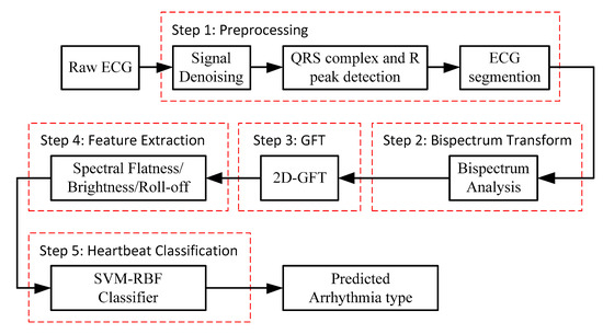
Figure 1.
Block diagram of the proposed method for ECG beat classification.
2.1. Pre-processing
The first step of our algorithm consisted of data pre-processing.
ECG signal can be contaminated by several artifacts, such as baseline wander, electromyographic artifacts and power frequency interferences [27,28]. These noises will affect the detection of real components and the classification of signal features. It is essential to figure out the suitable method for preprocessing while retaining the remarkable characteristics.
In the preprocessing stage, we used four steps to reduce noise. First, the DC component is eliminated by subtracting the average value. Then, the baseline drift is reduced with a median filter. The low-pass filter is used to remove power frequency interference and electromyogram (EMG) noise. Finally, the high-pass filter can eliminate some other low-frequency noise. After denoising, the R peak points are subsequently detected. The single heartbeat data are configured by segmenting the signal to be centered on the R peak point.
2.2. Bispectrum Analysis
After preprocessing, the single heartbeat data is analyzed by Bispectrum.
The HOS is one of the robust methods applied for the non-linear signal analysis. It depicts the spectra of third and higher order statistics (i.e., moments and cumulants). In this work, the third-order statistics (bispectrum) of the ECG signals are gathered [29].
The power spectrum of stochastic process is defined as the Fourier transform of auto-correlation function. Similarly, the high-order spectrum is defined as Fourier transform of high-order moment. The high-order spectrum is proposed to offer precise signal analysis and estimation, which may contain more details than low-order spectrum.
The minimum high-order spectrum is the bispectrum, a two-dimensional function of frequency, which is a very helpful tool to detect and quantify quadratic effects in time-series.
Denoting a stationary, zero mean and stochastic processes with third-order cumulant defined as
where and denote the time shift. denotes mathematical expectation.
Then, the bispectrum of is given by the expression
where , are two independent frequencies.
2.3. Graph Fourier Transform (GFT)
The Graph Fourier Transform (GFT) is the expansion of a graph signal function in terms of the eigenfunctions of the graph Laplacian matrix and is the foundation of GSP. The GFT is a data conversion method that is similar to the Fourier transform (FT).
After bispectrum analysis for the single heartbeat, the bispectrum results can be regarded as an image. We can execute 2D-GFT on the bispectrum results which is similar to execute 2D-FFT on images.
Superior to classical signal processing, graphs can be applied in irregular domains, so graph signal processing can be used to handle the irregular relationships between the data points [30].
An undirected graph usually includes the following three domain components: the vertex set , the edge set , and the weighted adjacency matrix . is the length of matrix row or column and also the number of vertices. Element is defined to show there is a connection between nodes and , otherwise . The matrix is the combination of elements .
Graph Laplacian matrix is defined by
where the th diagonal element in the diagonal matrix is defined by.
The real symmetric matrix has a complete set of orthonormal eigenvectors and the corresponding real eigenvalues , where the eigenvalues are all non-negative.
Vector can be used to represent the signal of the vertices of a graph, with the th component representing the signal value at the th vertex in .
The classical FT expands a continuous function considering the complex exponentials. Corresponding to FT, for a function , the GFT expands it in terms of the eigenvectors of the graph Laplacian domain. The GFT and inverse GFT of a graph signal are defined by Equations (5) and (6).
where quantifies the dependency of the vertex . represents the inner product of and . denotes convolution operation. From the definitions of the GFT and inverse GFT, the conservation equation of energy can be obtained as Equation (7).
where represents energy, denotes energy of signal, and denotes energy of eigenvalue spectral components.
In the 1D Euclidian Domain, the adjacency matrix is only affected by its precedent and ancient nodes. However, in 2D Euclidian Domain, the adjacency matrix is dominated by its precedent and ancient nodes both in rows and columns [31]. Meanwhile, the diagonal elements in the diagonal matrix are same as in the 1-D domain. For the th point data, the length and width of the adjacency matrix in 2D Euclidian Domain are .
In 2D Euclidian Domain, the index is bound with the row subscript and column subscript ,
The 2D-GFT and inverse 2D-GFT of a graph signal are defined by Equations (9) and (10).
where quantifies the dependency of the vertex .
2.4. Feature Extraction
After the 2D-GFT, spectral features can be extracted.
Finding the decisive features of the signals is a crucial step in the procedure. In the following subsections, spectral features are explained in detail. They are extracted from the spectral modes obtained using the bispectrum and 2D-GFT. Different spectral features, including spectral flatness, spectral brightness and spectral roll-off, were extracted from divided single heart beat [25].
Spectral flatness measures the distribution of power in all spectral bands. It is the ratio of the geometric mean to the arithmetic mean of the spectrum. In this paper, it has been extended into the two-dimensional case. Thus, the ratio is determined by the arithmetic and geometric mean both in rows and columns.
where is the absolute value.
The spectral flatness ranges from 0 to 1. The spectral flatness close to 0 means an extremely narrow band, while close to 1 means extraordinarily flat.
The spectral brightness is the ratio of sum of magnitudes of spectrum above a boundary to the total sum of all the magnitudes in the spectrum. Once determined, a big spectral brightness indicates the concentration of power in the band between and . The definition has also been expanded into a 2-D case, similar to the spectral flatness.
Spectral Roll-off is also a function corresponding to the boundary . Spectral roll-off can be used as the skewness which measures the non-uniformity of the signal about its mean value. In 2D-domain, the definition can be described as
where represents the coefficient.
2.5. Classifier
Support vector machine (SVM) is a popular supervised learning method which is widely used in pattern and object recognition, image processing and classification.
SVM can minimizes the empirical classification error by an optimal separating hyperplane, which can be represented by a decision function. In order to formulate the SVM algorithm based on radial basis function, we suppose a training set consists of samples , where denotes the data element and represents the corresponding class label. The decision function can be formulated as (14), (15)
Where is the product of the Lagrange multiplier, is the bias term, is the kernel function, and is kernel function parameter.
3. Experiment Setup
3.1. MIT-BIH Arrhythmia Database
The MIT-BIH Arrhythmia Database [26] is an internationally recognized database to evaluate the effectiveness and feasibility of proposed algorithms in the ECG signal processing field. The database consists of 48 real ECG recordings, including normal and abnormal beats. Each recording taken by two leads lasts for 30 min with a sampling rate of 360 Hz. Only the modified limb lead Ⅱ (ML Ⅱ) for each recording is used for the classification task. The recordings used in this paper can be found in the Supplementary Materials. Table 1 lists the detailed heartbeat types.

Table 1.
ECG class description using AAMI standard.
From the annotations of the database, five types of heart beats are included in the classification table. Four records (No.102, No.104, No.107 and No.217) were excluded because they contain paced heartbeats. We randomly selected 33 recordings from the remaining 44 records. Q class (unclassified and paced heartbeats) is discarded since this class is marginally represented in MIT-BIH database. Finally, the classification is only realized on other four classes (N, S, V and F) in our study. In our experiment, the cross-validation method and inter-patient scheme are used to measure classification performance.
In the cross-validation test, group of 75,604 heartbeats was randomly partitioned into 5 equal sized subsets (5-fold). From the 5 subsets, one is considered as the test-set for validating the trained model. The training set is constructed with the rest of subsets. This training and validation process is repeated 5 times performing the validation each time with a different subset.
In inter-patient scheme, all records are split into two groups (Training set & Testing set) with a proportion of the whole dataset. Grouping assignment is listed in Table 2.
Table 2.
Training set and testing set in inter-patient scheme.
3.2. Evaluation Metrics
To evaluate the classification performance, six classification metrics were used in this study. The metrics are defined by four concepts: true positive (), true negative (), false positive () and false negative (), respectively [32].
- Accuracy
Accuracy () is a relatively comprehensive evaluated guideline, directly reflecting the performance. It is the proportion of test examples classified correctly.
- Error rate
Error rate () is ratio of incorrect predictions over the total number of instances evaluated.
- Sensitivity
Sensitivity (), also called Recall, represents the probability that true positive samples can be correctly detected.
- Specificity
Specificity () means the percentage of correctly classified negative instances.
- Positive predictive rate
Positive predictive rate (), also called Precision, means the proportion of positive samples classified correctly.
- Macro-averaged F-score
Macro-averaged F-score () means relations between data’s positive labels and those given by a classifier based on a per-class average.
4. Experiments and Analysis
All the experiments were carried out using Matlab R2016a programming environment on a desktop Personal Computer (CW65S, Hasee Computer, Shenzhen, China) with Intel(R) Core i5-4210 CPU (2.60 GHz) and 8GB RAM configuration.
4.1. Pre-processing
ECG signal is easy to be interfered by several kinds of noises when collected. The common types of ECG signal noise are power frequency interference, baseline drift, and EMG noise [33]. Among them, EMG noise has a significant impact on ECG signal.
The MIT-BIH noise stress test database [34] offers EMG noise recording when assembling the ECG signal. The noise recordings were made using physically active volunteers and standard ECG recorders, leads, and electrodes; the electrodes were placed on the limbs in positions in which the subjects’ ECGs were not visible. The recordings are created by the script nstdbgen- using clean recordings from the MIT-BIH, to which calibrated amounts of noise from record ’em’ were added using nst- [26].
According to the requirement of Signal to Noise Ratio (SNR), ECG signal and noise of certain amplitude can be superposed. Here, two groups of ECG data with EMG noise, which SNR is 24 dB and 12 dB, are assembled as shown in Figure 2. There are fluctuations on original signals combined with EMG noises, and waves seems less smoothly with SNR declining.
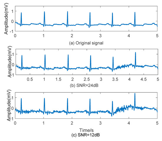
Figure 2.
Effect of EMG noise on ECG signal. (a) Original signal; (b) ECG signal with EMG noise (SNR = 24 dB); (c) ECG signal with EMG noise (SNR = 12 dB).
Several steps are conducted in noise reduction. First of all, the DC components are eliminated by subtracting the mean value. Baseline drift can be removed by a 8.33 ms width median filter. An 341th order low-pass filter using a Hanning window, whose cut-off frequency is 40 Hz, is used to remove power frequency interference and EMG noise. An 341th order high-pass filter using a Hanning window, whose cut-off frequency is 0.5 Hz, is used to remove some other low-frequency noise. Figure 3 demonstrates the ECG signal before and after denoising.
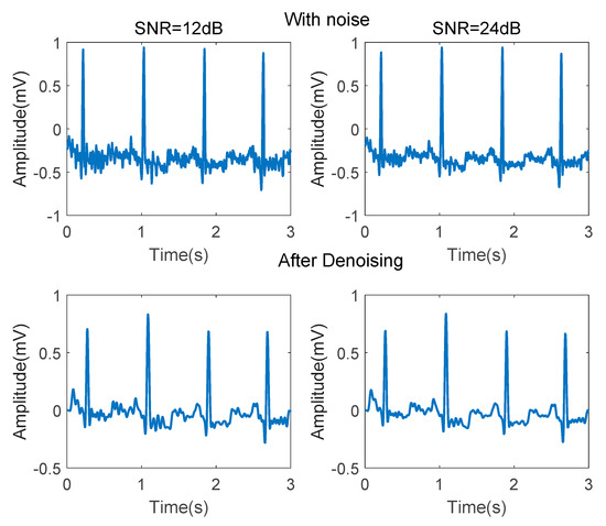
Figure 3.
ECG signals before and after denoising.
As shown in Figure 3, after denoising, the P-wave waveform, which is seriously disturbed by EMG noise, is significantly improved. Adaptive differential threshold method [35] is then conducted for QRS wave detection.
After detecting the R-peak in every QRS complex, the single heartbeat was segmented such that it was centered around the R peak, as shown in Figure 4. The segmentation length is 556 ms.
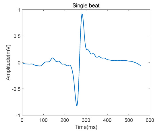
Figure 4.
Single heartbeat after denosing.
4.2. Transforming the ECG Signal into Bispectrum
Set the length of every segment as 128 and 50% as the overlapping rate. Figure 5 shows the bispectrum contour plots of the four types (N, S, V, and F beats) of ECG signals (from recordings No. 100, 232, 208 and 213).
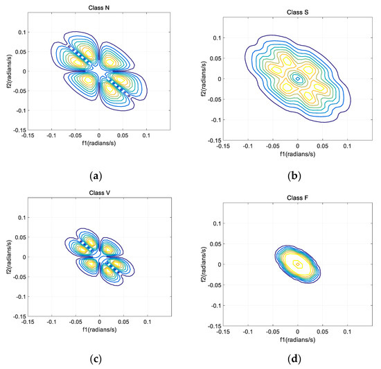
Figure 5.
Bispectrum contour plots of four segments in ECG records. (a) N beat (No. 100); (b) S beat (No. 232); (c) V beat (No. 208); (d) F beat (No. 213).
As shown in the Figure 5, due to the symmetrical characteristic of bispectrum, all information can be extracted from one part. Hence, only data in the first quadrant are recorded in this paper. There are no values in the upper triangle of the first quadrant and the lower triangle of the third quadrant of the dual-frequency plane, which corresponds to the undefined term of the bispectrum matrix.
Bispectrums of different beats have different contour shapes, therefore, the bispectrum can be considered as a feature. However, when bispectrum is used as a feature, matrices which contain much redundant information will be generated. So, bispectrum cannot be directly used as a feature of classification, and further feature extraction is needed. To solve this problem, various methods were proposed, including integral bispectrum [35], slice spectrum [29], Principal Component Analysis (PCA) [10], Independent Component Analysis (ICA) [36] and Kernel Fisher Discriminant Analysis (KFDA) [37].
4.3. 2D-GFT
In order to obtain high separability, the Graph Fourier Transform (GFT) of ECG signals is investigated from the graph spectrum domain. 2D-GFT helps enlarge the nuances among different classes. The impulse amplitude of the eigenvalue spectrum of the graph signal reflects the information of different components of the graph signal. The impulse amplitude of the eigenvalue is inversely proportional to the maximum value of the orthogonal eigenvector, that is, there are different degrees of amplification effects. With the increase of vertex number for graph signal, the maximum of orthonormal eigenvectors of Laplacian matrix will become smaller gradually. Effect of magnifying the difference should be more obvious [30].
The GFT matrix parameter is set to 64. Figure 6 is the whole mesh figure of four types (N, S, V & F beats) in ECG recordings. Figure 7 is top view of part of Figure 6.
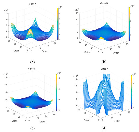
Figure 6.
Mesh plots of 4 types of ECG segments after 2D-GFT. (a) N beat (No. 100); (b) S beat (No. 232); (c) V beat (No. 208); (d) F beat (No. 213).
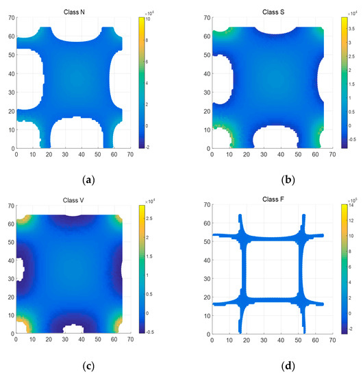
Figure 7.
Top view of 4 types of ECG segments after 2D-GFT (Z axis ranges from -5000 to 20000). (a) N beat (No. 100); (b) S beat (No. 232); (c) V beat (No. 208); (d) F beat (No. 213).
As shown in Figure 6, there is also the symmetrical characteristic in 2D-GFT results. In Figure 7, graphics change greatly with the transformation of types. In the enumerated range, the eigenvalue spectrum of Class V is much more complete than that of Class F in Figure 7. That means the values in Class V are relatively concentrated, Class S and Class N in the middle, then Class F the most decentralized. GFT helps expand the gap among all types.
GFT graph spectra distributions for the bispectrum of four types in ECG records are obviously different in the same region, the features can be extracted according to this characteristic.
4.4. Spectral Feature
4.4.1. Parameter Analysis in Spectral Features
The following content introduces the determination of parameters and . is used as evaluation metrics. The higher , the better the performance of the parameter.
In four types of beats (N, S, V and F), we can randomly select 500 samples from each type. The total number of the samples is 2000.
Since the eigenvalue matrix has symmetry and the values in first columns of the matrix are too small, so the boundary is set from 17, second half of matrix.
To determine the optimal boundary in spectral brightness, 15 experiments have been performed on different boundary values. Figure 8a shows the results under varied boundary from 17 to 31. The recognition rate reaches up to the highest when is 25, which is 94.7%. There’s a slight decline around 25. And is the lowest value when is 31, that’s because most power are concentrated before the boundary, leaving little room for fluctuation.
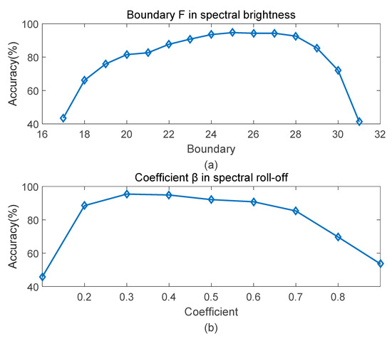
Figure 8.
Accuracy curve at different parameters. (a) boundary F; (b) coefficient β.
Similar to the boundary in spectral brightness, with same number of samples, coefficient in spectral roll-off is also determined by several experiments. As shows in Figure 8b, results change with increasing parameters (0.1 to 0.9). Accuracy reaches up to the peak when the coefficient is 0.3, which is 95.4%. Higher or lower coefficients both lead to the decrease of recognition rate.
4.4.2. Feature Extraction
On the basis of the bispectrum and 2D-GFT, more distinguishing features can be obtained. The spectral flatness, spectral brightness and spectral roll off are calculated. Results are present in Figure 9 and Figure 10.
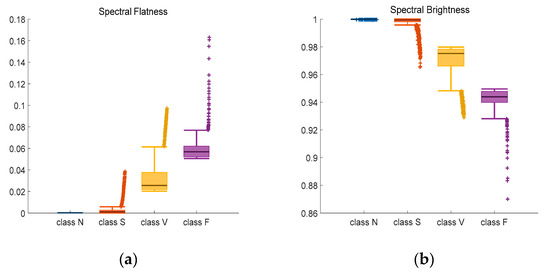
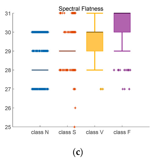
Figure 9.
Adjusted Boxplot of spectral features of N, S, V & F beats after bispectrum. (a) Spectral Flatness; (b) Spectral Brightness; (c) Spectral Roll-off.
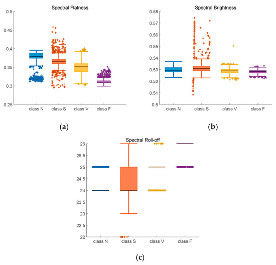
Figure 10.
Adjusted boxplot of spectral features of N, S, V, and F beats after bispectrum and 2D-GFT. (a) Spectral Flatness; (b) Spectral Brightness; (c) Spectral Roll-off.
Figure 9 is the combination of three spectral features of bispectrum of Class N, Class S, Class V, and Class F. The central line indicates the median value, and top and bottom edges indicate the maximum and minimum value respectively. Symbol ‘+’ are outliers. Figure 9a shows the spectral flatness values mainly range from 0 to 0.18, and the median value of Class N and Class S is lower than Class V and Class F. In Figure 9b, most values are close to 1. There is an obvious distinction between the spectral brightness of Class F and other three classes. Class F signals can be discriminated based on spectral brightness. Because the measure of the right skewness of the signal is the roll-off of the spectrum, most of the energy contained in the spectral coefficients is concentrated to the right of the average. It can be seen from the Figure 9c that the median value of the spectral roll-off of class F is the largest, about 30.6, while the median value of class N is the smallest, about 28.5. Spectral roll-off is the key factor to raise recognition rate.
Data listed in Table 3 are confidence interval (CI = 95%) of three kinds of features. For instance, the probability of a selected sample’s spectral flatness falling in interval [0.0101, 0.0106] is 95%. Compared with other classes, class N has the closest upper and lower bounds, which means little fluctuation.
Table 3.
CI (95%) of spectral features of N, S, V & F beats after bispectrum.
Figure 10 contains the spectral feature after 2D-GFT. In Figure 10a, median spectral flatness values are between 0.35 to 0.36 for Class N, 0.36 to 0.37 for Class S, 0.34 to 0.35 for Class V and 0.31 to 0.32 for Class F. Compared with Figure 9a, the value in Figure 10a is more distinguishable. In Figure 10b, median spectral brightness values of three classes are near 0.53, only value of class V is above it. The boxplot of Figure 10c is more concentrated than that of Figure 9c, the median spectral roll-off values of three classes are 25, 24, 25 and 26 with less outliers (+) outside the top and bottom edges.
Table 4 contains the confidence intervals of four classes after bispectrum and 2D-GFT. Similarly to those in Table 3, the indexes of class N are the most stable.
Table 4.
CI (95%) of spectral features of N, S, V & F beats after bispectrum+2D-GFT.
4.5. Classification Results
The classification refers to distinguishing different types of arrhythmias. In this section, SVM-RBF classifier was used to measure classification performance in cross-validation and inter-patient scheme. The penalty coefficient of SVM-RBF is 5 and the parameter gamma is 8.
4.5.1. Cross-validation Test
The whole amount of the heartbeats used for cross-validation is 75,604. Numbers of different types of heartbeat are shown in Table 5.
Table 5.
Number of different classes samples in cross-validation.
Table 6 is the average confusion matrix of classification results after merely bispectrum. Take N beats in Table 6 as an example, 89.95% beats are correctly classified on average, 10.05% beats are misclassified into Class S, Class V and Class F.
Table 6.
Average Confusion matrix of ECG heartbeat classification results after bispectrum in cross-validation.
Table 7 shows the metrics values measuring the classification performance associated to each class, including average value and standard deviation (SD). The method gives a high value of correct rate in executing arrhythmia classification, which is above 89.3%. Among all classes, standard deviation keeps below 0.245. Take F beats in Table 7 as an example, the is 96.9%, the is 3.1%, and the SD is 0.002.
Table 7.
Average Metrics of ECG heartbeat classification results after bispectrum in cross-validation.
Table 8 is the average confusion matrix of classification results after bispectrum and 2D-GFT. Also take N beats as an example, 96.28% beats are correctly classified on average, 3.72% beats are misclassified into Class S, Class V and Class F. Compared with the corresponding ones in Table 6, data in Table 8 get a remarkable improvement, about 5% for each class.
Table 8.
Confusion matrix of ECG heartbeat classification results after bispectrum+2D GFT in cross-validation.
Table 9 shows the metrics values after bispectrum+2D GFT. Also take F beats as an example, the is 98.8%, the is 1.2%, and the SD is 0.1%. Compared with Table 7, the indicators in Table 9 are better.
Table 9.
Average Metrics of ECG heartbeat classification results after bispectrum + 2D GFT in cross-validation.
Data listed in Table 10 and Table 11 is a more direct presentation of the proposed method compared with the results in the experiments conducted by [38,39,40,41,42,43,44]. All papers in Table 10 and Table 11 use the cross-validation method. The methods mentioned in Table 10 all use feature-extraction-pattern, the ones in Table 11 are not. The recordings used in other references listed in Table 10 and Table 11 are all from MIT-BIH database. However, the records and segments used in the training set and test set in each literature are not exactly the same. For example, a total of 46 records were used by Hui Yang et al. [38], except recordings No.102 and No.104 which have no lead II information. Huang et al. [43] used 14 recordings for classification, and for each type of the ECG signal, a segment of 10 seconds were selected.
Table 10.
Comparison with other existing approaches in cross-validation.
Table 11.
Comparison with non-feature-extraction-pattern classification approaches.
According to Hui Yang et al. [38], the combination of Parameter and Visual Pattern of ECG signals reached 97.70% of accuracy. Leandro B. Marinho et al. divided 100,467 heartbeats into 5 categories with an accuracy rate of 89.0% [39]. Paweł Pławiak [40] used the best evolutionary neural system based on SVM classifier to classify the data of 17 categories, then obtained an average accuracy of 90.20%. The methods proposed by Zhang et al. [41] and Zhang et al. [42] in previous years were Multi-lead fused method and ECG Morphology, respectively, achieving an accuracy of 86%. Huang et al. proposed a combination of STFT-Based Spectrogram and Convolutional Neural Network to achieve an accuracy of 99.0% [43]. Shu Lih Oh et al. [44], got an accuracy of 98.1% when combined the automated system of CNN and LSTM to analyze ECG signals. In this paper, we propose a method of combining 2D-GFT with bispectrum, which achieves 96.2% accuracy.
In our results, the average accuracy of merely bispectrum is only 87.8%, lower than most of methods listed in this Table 10. But when combined with 2D-GFT, the proposed method yields a higher average accuracy of this experiment to 96.2%, which suggests the method is a promising one in cross-validation.
Table 12 contains the detailed values of the proposed method in this section. After 2D-GFT, all metrics are improved. Especially, is improved by more than 30%. By our designed method, the , and of the S beats are 71.5%,99.3% and 82.6%, those of the V beats are 76.7%, 99.2% and 86.9%, those of the F beats are 46.2%, 99.9% and 91.0%, respectively.
Table 12.
Classification results on class S, class V, and class F.
The time cost of each method is listed in Table 13 which represents the time for one heartbeat to process. The running time of bispectrum combined with 2D-GFT is longer because of the higher algorithmic complexity and better performance of detection, which matches our anticipation. The 2D-GFT is very time consuming because of varied parameters.
Table 13.
Computational complexity analysis.
4.5.2. Test in Inter-patient Scheme
The second experiment is based on inter-patient scheme, detailed numbers are listed in Table 14.
Table 14.
The number of ECG beats used for training and testing sets on inter-patient scheme.
Table 15 shows the confusion matrix of the classification results on the testing set in inter-patient scheme. 1371, 1643 and 296 Class N samples are misclassified into other three classes separately. Class N is still the main misclassification destination for other three classes.
Table 15.
Confusion matrix of ECG heartbeats classification results after bispectrum +2D-GFT on inter-patient scheme.
Results quoted in Table 16 are the comparison of the results conducted by Afkhami et al. [7], Zhang et al. [42], Ye et al. [45] and the proposed method. The overall accuracy is improved to 92.2%, higher than any other related literature. Besides, and get a remarkable improvement in this experiment. For instance, the specific of S beats is 99.7%, much higher than the methods proposed by Afkhami et al. [7] and Ye et al. [45], and 5.8% higher than method proposed by Zhang et al. [42]. It demonstrates that the proposed method in this paper is a reliable tool in detecting the arrhythmia signals.
Table 16.
Comparison with other existing approaches on inter-patient scheme.
5. Conclusions
The aim of the conducted research is to develop a new methodology that enables the efficient classification of cardiovascular disease. The ECG signals can be tool for the medical practitioners to detect various types of cardiac arrhythmia because abnormal heart electrical activity can cause irregular morphology changes which would be checked through ECG signals.
In this paper, we proposed an ECG arrhythmia analysis method based on the combination of bispectrum and 2D-GFT. In the proposed method, we use high-order spectra to detect the basic features and then execute 2D-GFT on the result. And extract 2D spectral features. Support vector machine based on the RBF kernel are employed in the classification procedure. The experimental results depicted that our proposed model achieved a high classification accuracy of 96.2%. The novelty of this approach is to regard the bispectrum results as an image and apply 2D-GFT to the ECG signal. Compared with the previous references, such as Acharya [10] and Zhelin [17], our advantage is that we can achieve effective classification using only three features, which greatly improves the classification efficiency. Furthermore, the methods used by Acharya et al. [10] and Zhelin et al. [17] only made binary classification, while the proposed method can achieve multi-class categorization. Compared with Zhang et al. [41], who also used three features for classification, the accuracy of our method is 10% higher than theirs.
ECG recordings of four arrhythmia types, shared by the MIT-BIH arrhythmia database, were used for evaluations of the algorithm performance. We used the cross-validation method for classification. Compared with bispectrum analysis, after 2D-GFT, all metrics are improved. By our designed method, the sensitivity, specificity and positive predictive rate of the S beats are improved 30.5%, 0.3% and 8.3%, those of the V beats are improved 26.9%, 9.7% and 9.7%, those of the F beats are improved 27.2%, 0.4% and 36.4%, respectively. Comparisons with peer works prove a marginal progress in heart arrhythmia classification performance. This study proves that the proposed method is an excellent model for the diagnosis of heart diseases based on ECG signals.
In comparison with some references, the data pre-processing process in this paper is comparative to recent approaches, which may affect the classification effect of the ECG signals. Many methods have been proposed to remove noise, such as wavelet transform [46], empirical mode decomposition [47], independent component analysis [48,49], and so on. In future work, we can improve the pre-processing method to achieve better classification effect.
Deep learning is the focus of current research and has been successfully applied in the classification of ECG signals. For example, Leandro et al. [38] got an accuracy of 97.7% with a classifier of KNN. We can combine our method with neural networks to realize the classification of more types of ECG signals later. Furthermore, the approach proposed in this paper could be extended to solve the imbalance problem in other related fields.
Supplementary Materials
The MIT-BIH arrhythmia database can be found at the following website: https://www.physionet.org/content/mitdb/1.0.0/. The data used in this paper including record 100, 101, 103, 109, 111, 112, 113, 115, 116, 117, 118, 121, 122, 123, 124, 200, 202, 205, 208,209, 210, 212, 213, 214, 215, 219, 220, 221, 222, 223, 230, 231, 232.
Author Contributions
S.L. and J.S. designed the algorithms, performed the experiments, and analyzed the experimental data. T.K. and R.M. contributed in data analysis, checking and correcting and R.M. co-supervised the students. All authors have read and agreed to the published version of the manuscript.
Funding
This research was funded by Open Research Fund of Key Laboratory of Ministry of Education (UASP1604).
Conflicts of Interest
The authors declare no conflict of interest.
References
- Wang, H.; Naghavi, M.; Allen, C.; Barber, R.M.; Bhutta, Z.A. Global, regional, and national age–sex specific all-cause and cause-specific mortality for 240 causes of death, 1990–2013: A systematic analysis for the Global Burden of Disease Study 2013. Lancet 2015, 385, 117–171. [Google Scholar]
- Hemmeryckx, B.; Feng, Y.; Frederix, L.; Lox, M.; Trenson, S.; Vreeken, R.; Lu, H.R.; Gallacher, D.; Ni, Y.; Lijnen, H.R. Evaluation of cardiac arrhythmic risks using a rabbit model of left ventricular systolic dysfunction. Eur. J. Pharm. 2018, 832, 145–155. [Google Scholar] [CrossRef] [PubMed]
- Zipes, D.P. Clinical application of the electrocardiogram. J. Am. Coll. Cardiol. 2000, 36, 1746–1748. [Google Scholar] [CrossRef]
- Madeiro, J.P.V.; Cortez, P.C.; Oliveira, F.I.; Siqueira, R.S. A new approach to QRS segmentation based on wavelet bases and adaptive threshold technique. Med. Eng. Phys. 2007, 29, 26–37. [Google Scholar] [CrossRef]
- Chazal, P.; O’Dwyer, M.; Reilly, R.B. Automatic classification of heartbeats using ECG morphology and heartbeat interval features. IEEE Trans. Biomed. Eng. 2004, 51, 1196–1206. [Google Scholar]
- Llamedo, M.; Martínez, J.P. Heartbeat classification using feature selection driven by database generalization criteria. IEEE Trans. Biomed. Eng. 2011, 58, 616–625. [Google Scholar] [CrossRef]
- Afkhami, R.G.; Azarnia, G.; Tinati, M.A. Cardiac arrhythmia classification using statistical and mixture modeling features of ECG signals. Pattern Recognit. Lett. 2016, 70, 45–51. [Google Scholar] [CrossRef]
- Kaur, H.; Rajni, R. On the detection of cardiac arrhythmia with principal component analysis. Wirel. Pers. Commun. 2017, 97, 5495–5509. [Google Scholar] [CrossRef]
- Homaeinezhad, M.R.; Atyabi, S.; Tavakkoli, E.; Toosi, H.N.; Ghaffari, A.; Ebrahimpour, R. ECG arrhythmia recognition via a neuro-SVM-KNN hybrid classifier with virtual QRS image-based geometrical features. Expert Syst. Appl. 2012, 39, 2047–2058. [Google Scholar] [CrossRef]
- Acharya, U.R.; Sudarshan, V.K.; Koh, J.E.; Martis, R.J.; Tan, J.H.; Oh, S.L.; Muhammad, A.Y.; Hagiwara, M.; Mookiah, R.K.; Chua, K.P.; et al. Application of higher-order spectra for the characterization of coronary artery disease using electrocardiogram signals. Biomed. Sign. Process. Control 2017, 31, 31–43. [Google Scholar] [CrossRef]
- Raj, S.; Ray, K.C. Sparse representation of ECG signals for automated recognition of cardiac arrhythmias. Expert Syst. Appl. 2018, 105, 49–64. [Google Scholar] [CrossRef]
- Ye, C.; Coimbra, M.T.; Kumar, B.V. Arrhythmia detection and classification using morphological and dynamic features of ECG signals. In Proceedings of the 2010 Annual International Conference of the IEEE, Buenos Aires, Argentina, 31 August–4 September 2010; pp. 1918–1921. [Google Scholar]
- Xu, S.S.; Mak, M.; Cheung, C. Towards End-to-End ECG classification with raw signal extraction and deep neural networks. IEEE J. Biomed. Health Inform. 2019, 23, 1574–1584. [Google Scholar] [CrossRef] [PubMed]
- Matta, S.C.; Sankari, Z.; Rihana, S. Heart rate variability analysis using neural network models for automatic detection of lifestyle activities. Biomed. Sign. Process. Control 2018, 42, 145–157. [Google Scholar] [CrossRef]
- Christopher, K.K.; Matthew, A.H. Decomposition of higher-order spectra for blind multiple-input deconvolution, pattern identification and separation. Signal. Process. 2019, 165, 357–379. [Google Scholar]
- Xun, C.; Aiping, L.; Qiang, C.; Yu, L.; Liang, Z.; Martin, J.; McKeown, M.J. Simultaneous ocular and muscle artifact removal from EEG data by exploiting diverse statistics. Comput. Biol. Med. 2017, 88, 1–10. [Google Scholar]
- Zhelin, Y.; Sungnien, Y. Bispectrum and Histogram Features for the Identification of Atrial Fibrillation Based on Electrocardiogram. In Proceedings of the 40th Annual International Conference of IEEE Engineering in Medicine and Biology Society, Honolulu, HI, USA, 17–22 July 2018; pp. 5994–5997. [Google Scholar]
- Mitra, S.; Mitra, M.; Chaudhuri, B.B. Pattern defined heuristic rules and directional histogram based online ECG parameter extraction. Measurement 2008, 42, 150–156. [Google Scholar] [CrossRef]
- Spielman, D. Spectral Graph. Theory; Betascript Publishing: Missoula, MT, USA, 2010. [Google Scholar]
- Khatua, M.; Safavi, S.H.; Cheung, N. Sparse Laplacian Component Analysis for Internet Traffic Anomalies Detection. IEEE Trans. Sign. Inform. Process. Netw. 2018, 4, 697–711. [Google Scholar] [CrossRef]
- Hosseinalipour, S.; Wang, J.; Tian, Y.; Dai, H. Infection Analysis on Irregular Networks through Graph Signal Processing. IEEE Tran. Netw. Sci. Eng. 2018, 8, 1–13. [Google Scholar] [CrossRef]
- Wang, J.; Calhoun, V.; Stephen, J.M.; Wilson, T.W.; Wang, Y. Integration of network topological features and graph Fourier transform for fMRI data analysis. In Proceedings of the 2018 IEEE 15th International Symposium on Biomedical Imaging (ISBI 2018), Washington, DC, USA, 4–7 April 2018; pp. 92–96. [Google Scholar]
- Shuman, D.I.; Ricaud, B.; Vandergheynst, P. Vertex-frequency analysis on graphs. Comput. Harmon. Anal. 2016, 40, 260–291. [Google Scholar] [CrossRef]
- Shafipour, R.; Khodabakhsh, A.; Mateos, G.; Nikolova, E. A Directed Graph Fourier Transform with Spread Frequency Components. IEEE Trans. Sign. Process. 2019, 67, 946–960. [Google Scholar] [CrossRef]
- Satija, U.; Trivedi, N.; Biswal, G.; Ramkumar, B. Specific Emitter Identification Based on variational mode decomposition and spectral features in single hop and relaying scenarios. IEEE Trans. Inf. Forensics Secur. 2019, 14, 581–591. [Google Scholar] [CrossRef]
- Mark, R.; Moody, G. MIT-BIH Arrhythmia Database Directory; MIT Press: Cambridge, MA, USA, 1988. [Google Scholar]
- Xu, X.; Liu, H. ECG Heartbeat Classification Using Convolutional Neural Networks. IEEE Access 2020, 8, 8614–8619. [Google Scholar] [CrossRef]
- Israel, S.A.; Irvine, J.M.; Cheng, A.; Wiederhold, M.D.; Wiederhold, B.K. ECG to identify individuals. Pattern Recognit. 2005, 38, 133–142. [Google Scholar] [CrossRef]
- Cai, J.; Li, X. Gear Fault Diagnosis Based on Empirical Mode Decomposition and 1.5 Dimension Spectrum. Shock Vib. 2016, 3, 1–10. [Google Scholar] [CrossRef]
- Lu, O.; Yu, D.; Yang, H. A new rolling bearing fault diagnosis method based on GFT impulse component extraction. Mech. Syst. Sign. Process. 2016, 81, 162–182. [Google Scholar]
- Chindanur, N.B.; Sure, P. Low Dimensional Models for Traffic Data Processing using Graph Fourier Transform. Comput. Sci. Eng. 2018, 20, 24–37. [Google Scholar] [CrossRef]
- Marina, S.; Guy, L. A systematic analysis of performance measures for classification tasks. Inf. Process. Manag. 2009, 45, 427–437. [Google Scholar]
- Ren, A.F.; Du, Z.X.; Li, J. Adaptive interference cancellation of ECG signals. Sensors 2017, 17, 942. [Google Scholar] [CrossRef] [PubMed]
- Moody, G.B.; Muldrow, W.E.; Mark, R.G. A noise stress test for arrhythmia detectors. Comput. Cardiol. 1984, 11, 381–384. [Google Scholar]
- Jiang, J.; Zhang, H.; Pi, D.; Dai, C. A novel multi-module neural network system for imbalanced heartbeats classification. Expert Syst. Appl. X 2019, 1, 1–15. [Google Scholar] [CrossRef]
- Chandran, V.; Elgar, S.L. Pattern Recognition Using Invariants Defined From Higher Order Spectra-One Dimensional Inputs. IEEE Tran. Sign. Process. 1993, 41, 205–212. [Google Scholar] [CrossRef]
- Dhir, C.S.; Lee, S. Discriminant Independent Component Analysis. IEEE Trans. Neural Netw. 2011, 22, 845–857. [Google Scholar] [CrossRef] [PubMed]
- Hui, Y.; Zhiqiang, W. Arrhythmia Recognition and Classification Using Combined Parametric and Visual Pattern Features of ECG Morphology. IEEE Access 2020, 8, 47103–47117. [Google Scholar]
- Leandro, B.M.; Navar, D.M.M.N.; João, W.M.S.; Mateus, V.G.; Pedro, P.R.F.; Victor, H.C.D.A. A novel electrocardiogram feature extraction approach for cardiac arrhythmia classification. Future Gener. Comput. Syst. 2019, 97, 564–577. [Google Scholar]
- Pawel, P. Novel methodology of cardiac health recognition based on ECG signals and evolutionary-neural system. Expert Syst. Appl. 2018, 92, 334–349. [Google Scholar]
- Zhang, Z.; Luo, X. Heartbeat Classification Using Decision Level Fusion. Biomed. Eng. Lett. 2014, 4, 388–395. [Google Scholar] [CrossRef]
- Zhang, Z.; Dong, J.; Luo, X.; Choi, K.S.; Wu, X. Heartbeat classification using disease-specific feature selection. Comput. Biol. Med. 2014, 46, 79–89. [Google Scholar] [CrossRef]
- Huang, J.S.; Chen, B.Q.; Yao, B. ECG Arrhythmia classification using STFT-based spectrogram and convolutional neural network. IEEE Access 2019, 7, 92871–92880. [Google Scholar] [CrossRef]
- Shu, L.O.; Eddie, Y.K.; Ng, R.; SanTan, U.; Rajendra, A. Automated diagnosis of arrhythmia using combination of CNN and LSTM techniques with variable length heart beats. Comput. Biol. Med. 2018, 102, 278–287. [Google Scholar]
- Ye, C.; Vijaya, K.B.V.K.; Coimbra, M.T. Heartbeat classification using morphological and dynamic features of ECG signals. IEEE Trans. Biomed. Eng. 2012, 59, 2930–2941. [Google Scholar]
- Wang, L.; Sun, W.; Chen, Y.; Li, P.; Zhao, L. Wavelet transform based ECG denoising using adaptive thresholding. In Proceedings of the 7th International Conference on Bioinformatics and Biomedical Science (ICBBS), Shenzhen, China, 23–25 June 2018; pp. 35–40. [Google Scholar]
- Rakshit, M.; Das, S. An efficient ECG denoising methodology using empirical mode decomposition and adaptive switching mean filter. Biomed. Signal Process. Control 2018, 40, 140–148. [Google Scholar] [CrossRef]
- He, T.; Clifford, G.; Tarassenko, L. Application of independent component analysis in removing artefacts from the electrocardiogram. Neural Comput. Appl. 2006, 15, 105–116. [Google Scholar] [CrossRef]
- Johan, W.; Reza, M.; Gerhard, H. Wireless Capacitive-Based ECG Sensing for Feature Extraction and Mobile Health Monitoring. IEEE Sens. J. 2018, 18, 6023–6032. [Google Scholar]


© 2020 by the authors. Licensee MDPI, Basel, Switzerland. This article is an open access article distributed under the terms and conditions of the Creative Commons Attribution (CC BY) license (http://creativecommons.org/licenses/by/4.0/).