Article

Novel Swarm Intelligence Algorithm for Global Optimization and Multi-UAVs Cooperative Path Planning: Anas Platyrhynchos Optimizer

1
Research Institute of Pilotless Aircraft, Nanjing University of Aeronautics and Astronautics, Nanjing 210016, China
2
Key Laboratory of Unmanned Aerial Vehicle Technology, Ministry of Industry and Information Technology, Nanjing University of Aeronautics and Astronautics, Nanjing 210016, China
3
College of Automation Engineering, Nanjing University of Aeronautics and Astronautics, Nanjing 210016, China
4
College of Astronautics, Nanjing University of Aeronautics and Astronautics, Nanjing 210016, China
*
Authors to whom correspondence should be addressed.
Appl. Sci. 2020, 10(14), 4821; https://doi.org/10.3390/app10144821
Submission received: 8 June 2020 / Revised: 30 June 2020 / Accepted: 8 July 2020 / Published: 14 July 2020

Abstract

:
In this study, a novel type of swarm intelligence algorithm referred as the anas platyrhynchos optimizer is proposed by simulating the cluster action of the anas platyrhynchos. Starting from the core of swarm intelligence algorithm, on the premise of the use of few parameters and ease in implementation, the mathematical model and algorithm flow of the anas platyrhynchos optimizer are given, and the balance between global search and local development in the algorithm is ensured. The algorithm was applied to a benchmark function and a cooperative path planning solution for multi-UAVs as a means of testing the performance of the algorithm. The optimization results showed that the anas platyrhynchos optimizer is more superior in solving optimization problems compared with the mainstream intelligent algorithm. This study provides a new idea for solving more engineering problems.

1. Introduction

The swarm intelligence algorithm is an important optimization method. This type of algorithm is highly suitable for problems that are difficult to be solved effectively or even cannot be solved by traditional technology, as establishing an effective formal model, such as NP-hard problems, is difficult to accomplish. The traveling salesman problem (TSP) is one of the most classical NP-hard problems. In TSP, a traveling salesman is expected to identify the shortest path to visit n cities in a country. Suppose that the traveling salesman arrives at a country with only 21 cities and visits the cities in any order (from one city and moves directly to another city), the size of the search space in this problem can be calculated as ( n 1 ) ! . This formulation suggests that the TSP with n = 21 entails 2.432902 × 10 18 possible travel searches. If a person takes one second to calculate a single travel, then 770 million years are needed to search the whole search space. If a computer with a 2.0 GHz CPU (i.e., 2 billion instructions per second) is used, then 38 years are required to identify all possible paths. If a city is added to this problem, then the time is increased accordingly to nearly 810 years. However, Reference [1] has shown that the swarm intelligence algorithm is outstanding in solving these problems. Consequently, the swarm intelligence algorithm has become widely popular among researchers in recent years.
The swarm intelligence algorithm is inspired by the behavior of social creatures such as ants, termites, birds, and fish. The most popular swarm intelligence algorithm at the beginning of algorithm development is particle swarm optimization (PSO). The PSO algorithm [2] was proposed by Kennedy and Eberhart, and it was inspired by the social behavior of birds. With the popularization and development of the swarm intelligence concept, a variety of swarm intelligence algorithms have been proposed in succession, namely, ant colony optimization (ACO) [3], bat algorithm (BA) [4], dragonfly optimization [5], grasshopper optimization algorithm (GOA) [6], moth flame optimization algorithm (MFOA) [7], gray wolf optimization (GWO) [8], and whale optimization algorithm (WOA) [9], all of which have been widely used in recent years. Nature is the infinite source of inspiration in computational science, and more swarm intelligence algorithms are expected in the future.
Swarm intelligence algorithms have been widely applied to various practical engineering issues in recent years. Whale optimization algorithm, which was proposed in 2016, has been cited more than 1600 times as of April 2020 based on Google Scholar indicators and has been widely used in different fields such as energy [10,11], computer networks [12,13], cloud computing [14], image processing and machine vision [15,16], electronics and electrical engineering [17,18], antenna design [19], feature selection [20,21,22], aerospace [23], path planning [24], and structural optimization [25,26]. Moreover, GOA has been successfully applied to the trajectory optimization of multiple solar-powered UAVs [27], short-term load forecasting [28], electrical characterization of proton exchange membrane fuel cell stacks [29], data clustering [30], scheduling of thermal system [31], analyzing vibration signals from rotating machinery [32], short-term wind electric power forecasting [33], optional distribution system reconfiguration and distributed generation placement [34], classification for biomedical purpose [35], design of linear antenna arrays [36], automatic seizure detection of EEG signals [37], designing automatic voltage regulator systems [38], training neural network [39], and other issues. The multiverse optimizer (MVO) algorithm has also been widely used in different fields. In References [40,41], MVOs were used to train multilayer perceptron neural networks. Benmessahel [42] combined the MVO and the artificial neutral network to develop an intrusion detection system. In Reference [43], the MVO was used to optimize the parameters of support vector machines. Rosenberg [44] solved the clustering problem by using the search ability of the MVO. Thus far, the studies conducted indicate that swarm intelligence algorithms can effectively solve many practical optimization problems.
The no free lunch (NFL) theorem [45] has proven logically that swarm intelligence algorithms cannot be regarded the most suitable solution for all optimization problems. In other words, the specific swarm intelligence algorithm may perform effectively in one group of problems but not for another group of problems. In the case of GWO, the original version of GWO can solve problems by using continuous variables. On this basis, the algorithm can be modified to solve binary or discrete problems. Emary [46] proposed the combination of the evolutionary operator with GWO to solve binary problems. A similar evolutionary operator was used in the literature [47]. Jayabarathi [48] combined the crossover and mutation operators with GWO to solve economic scheduling problems. Additionally, the binary version of GWO inspired by quantum mechanics was also proposed in the literature [49]. Moreover, Liu [50] designed an initialization method based on the greedy idea and mutation and position update strategies by combining the dynamic weighted average with the static average to solve path planning problems, including the lack of GWO development ability and inflexible position update strategy. In terms of combining the advantages of different algorithms, the method that mixes multiple algorithms to improve performance has also been widely used. Singh [51] proposed the hybrid GWO and PSO optimization algorithm to improve convergence speed and the ability to determine global optimal values. Rashid [52] adopted a hybrid algorithm based on the ACO and GWO to optimize assembly sequence planning. ElGayyar [53] proposed a hybrid GWO and BA method to solve global function optimization problems. Pan [54] proposed a hybrid GWO and flower pollination algorithm to improve algorithm performance. The other combination optimization methods include GWO and DE [55], GWO and SCA [56], GWO and BBO [57], WOA and PSO [58], and WOA and BO [59]. The NFL theorem allows the research in the field of swarm intelligence to be extremely active, which is one of the important reasons why a large number of scholars have committed to improve the current algorithm and propose new swarm intelligence algorithms.
No existing algorithm in the reviewed literature simulates the behavior of anas platyrhynchos, hence, our attempt to model the behavior of this animal and design a new swarm intelligence algorithm based on the model. Inspired by the swarm behavior of anas platyrhynchos, this study proposes a novel swarm intelligence algorithm referred as the anas platyrhynchos optimizer (APO). In general, researchers pursue a lot of performance in order to improve performance. Although the performance is improved, the introduction of additional parameters not only complicates the algorithm, but also masks the core mechanism of the swarm intelligence algorithm to a certain extent. In this study, starting from the core of the cluster intelligence algorithm, we designed the APO algorithm period to have not only better performance but also as few parameters as possible. The performance of the algorithm was tested on 23 classical benchmark functions and compared with PSO, DE, WOA, and GWO, to verify the effectiveness of APO algorithm. To further verify the performance of the algorithm in practical engineering applications, APO was used to solve the cooperative path planning problem of multi-UAVs, and the results were compared with GWO, IGWO, HGWO, PSO, and DE algorithms. The main contributions of this paper are to propose a new SI technique with inspiration from the behavior of anas platyrhynchos. A new swarm intelligence algorithm is proposed, and its performance was verified in this paper. In addition, the algorithm was applied to solve the problem of multi-UAVs cooperative path planning, thereby demonstrating its potential in engineering applications and providing new solutions for other engineering optimization problems.
The structure of the rest of this paper is as follows: Section 2 describes in detail the anas platyrhynchos optimizer proposed in this study. Section 3 present the test problem and optimization results of the benchmark function optimization and the multi-UAV cooperative path planning. The main study contents are concluded, and the future study direction is proposed in Section 4.

2. Anas Platyrhynchos Optimizer

2.1. Inspiration

Anas platyrhynchos who prefer the group life usually live in groups on banks of freshwater lakes and in rivers, lakes, reservoirs, bays, and other water bodies. In summer, anas platyrhynchos in small groups inhabit freshwater rivers, lakes, and swamps where aquatic plants flourish. In autumn, they change their feathers and often gather in large groups of hundreds or even thousands of birds in migration. In addition, anas platyrhynchos live in a group of hundreds in winter.
American biologists have found that anas platyrhynchos have a habit of controlling parts of their brains to keep on sleeping and another part to keep them awake. Anas platyrhynchos can also open one eye and close the other eye during sleeping. This study provides the first evidence that animals can control their sleeping state. The half-asleep and half-awake habit of anas platyrhynchos help them evade predator animals in a dangerous environment. During gathering in crowds and groups of anas platyrhynchos, a leading duck can be observed in the anas platyrhynchos swarm, and other ducks will flock to the leading duck. As a result, the whole duck group will move towards the destination. When a single duck is out of the flock, the lone duck can find its companion by calling and moving towards them, eventually moving with the whole flock. As a group, anas platyrhynchos can coordinate themselves into the whole flock. This type of swarm intelligence can be associated with the target problem requiring optimization. Inspired by the collective behavior of anas platyrhynchos, a new swarm intelligence algorithm can be designed.
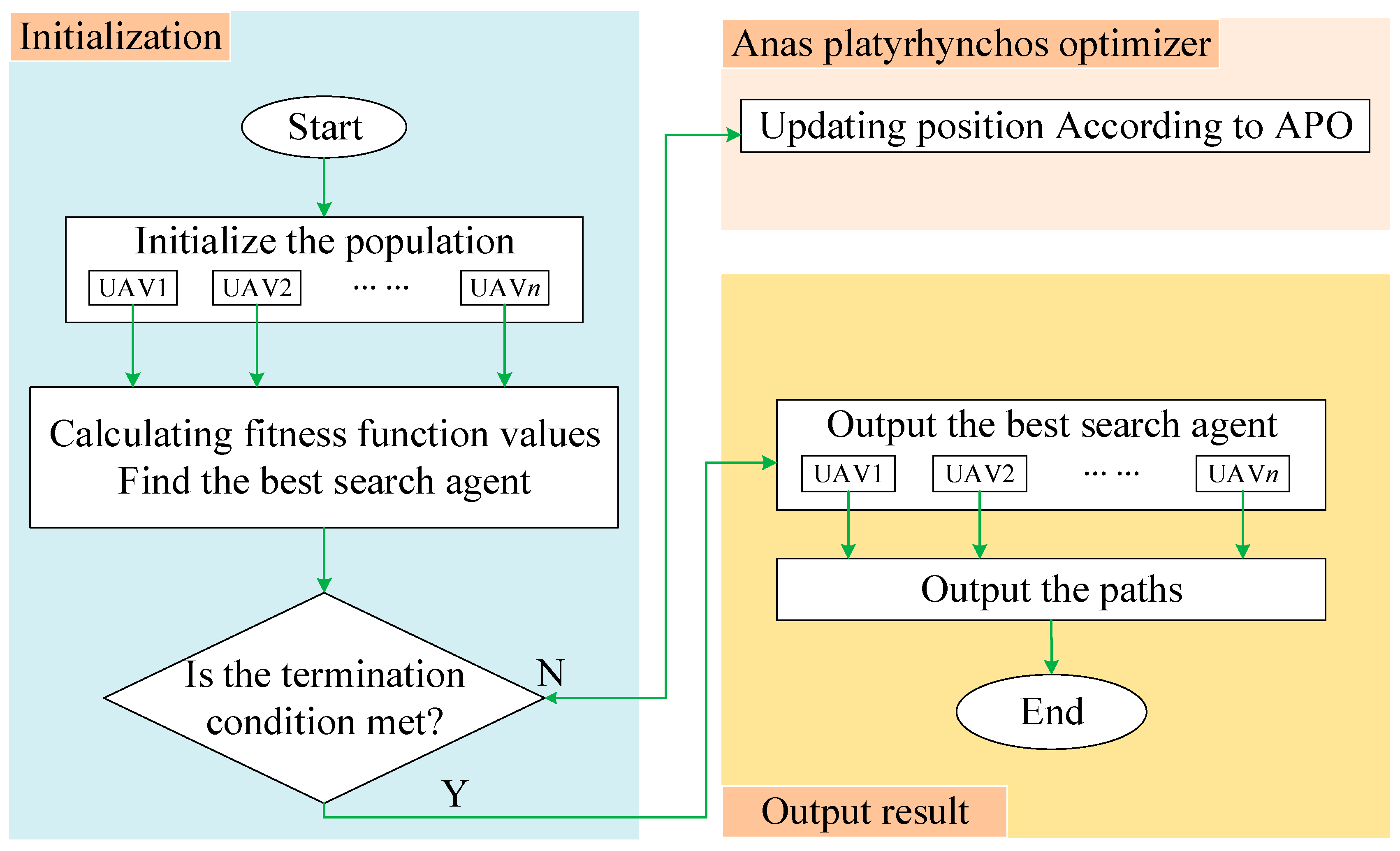
The anas platyrhynchos optimizer mainly stimulates the warning behavior and the moving process of anas platyrhynchos swarm. In solving optimization problems, each duck is regarded as an individual particle that can move freely, while several ducks form the duck flock. At the beginning, the anas platyrhynchos are randomly distributed in the search space. The duck with the best fitness function at present is considered the leading duck. As the following object of all ducks, the leading duck guides its companions to go with it, all anas platyrhynchos mainly go through two stages of warning and moving. The warning and sentry behavior of anas platyrhynchos and the moving process of the whole flock are shown in Figure 1. In the early warning stage, the danger degree of each particle is represented by the value of its fitness function. The lower the degree of danger, the lower the probability of flying in the presence of danger. When a duck is in distress, it will fly to the least dangerous leading duck. At the same time, each duck will fly towards the leading duck during the moving stage. If the fitness function value is worse after the flight, it means that the duck is separated from the swarm. At this time, the duck randomly selects one duck: If the fitness function value of the selected duck is lower than that of the stray duck, the stray duck flies to the selected duck; if the fitness function value of the selected duck is equal to the stray duck, the stray duck fails to find a partner; if the fitness function value of the selected duck is higher than that of the stray duck, it means that the selected duck is another stray duck and the selected duck also flies to the stray duck. In this study, a new swarm intelligence algorithm referred as the anas platyrhynchos optimizer was designed on the basis of the mathematical modeling of the warning behavior and the moving process.

2.2. Mathematical Model and Algorithm

In this section, we propose a novel swarm intelligence algorithm named anas platyrhynchos optimizer (APO) which contains two main behaviors: warning behavior and moving process.

2.2.1. Warning Behavior

Before the warning behavior, according to the anas platyrhynchos behavior model, the population in APO is initialized as follows:
P o p i = r a n d × ( u p l o w ) + l o w ,
where P o p i is the ith population, N is the population size, low and up are the lower and upper bounds of the search space, and rand is a random value selected from the range [0, 1].
In the warning behavior, the flying in danger operation realized by the select probability Pc is proposed. The main process of the warning behavior is introduced as follows.
Step 1: Calculate the probability of distress Pc by Equation (2).
P c i = r a n k ( f i t ( P o p i ) ) N ,
where f i t ( P o p i ) is the fitness value of P o p i and r a n k ( f i t ( P o p i ) ) is considered as the rank of the individual P o p i among the other individuals in the population.
Step 2: If the probability Pc is satisfied, generate the new individual by Equation (3).
P o p i ( t + 1 ) = P o p i ( t ) + s i g n ( r a n d 1 2 ) × α 0 × | P o p i ( t ) P o p b e s t ( t ) | × L e v y ( s ) ,
where t refers to the current iterations, and P o p b e s t is the leading duck, α 0 > 0 is the step length scale factor, and sign refers to the sign function. Levy flight provides the random walk for the Equation (6), and its distribution equation is expressed as Equation (4).
L e v y   ~   μ = t λ ,   1 < λ 3 .
Levy flight is a special type of random walk, and the probability distribution of its step length obeys a heavy-tailed distribution which is shown in Equation (5).
s = μ | ν | 1 β ,
where s refers to the Levy flight step length. Moreover, in Equation (4), λ = 1 + β , we use α 0 = 0.01 and β = 3 / 2 as CS set in [60]. μ and ν are selected from the normal distribution μ = N ( 0 , δ μ 2 ) and ν = N ( 0 , δ ν 2 ) , where
δ μ = [ Γ ( 1 + β ) sin ( π β / 2 ) β × Γ ( ( 1 + β ) / 2 ) × 2 ( β 1 ) / 2 ] 1 β δ ν = 1

2.2.2. Moving Process

Reference [61] describes an intelligent algorithm for simulating biological migration. Compared with the self-organizing migration algorithm [61] (SOMA), APO mainly focus on the anas platyrhynchos, imitates its migration movement and models it. It is completely different from the location update strategy and algorithm flow in SOMA. In this behavior of APO, the main process is introduced as follows.
Step 1: After the optimal particle is defined, other search particles will attempt to move to the optimal particle. The mathematical model of this behavior is given by Equation (7).
P o p i ( t + 1 ) = P o p i ( t ) A | C × P o p b e s t ( t ) P o p i ( t ) | ,
where A and C refer to the coefficient vector, which can be obtained from Equations (8) and (9).
A = 2 a × r a n d a ,
C = 2 × r a n d ,
where a refers to a coefficient vector that linearly decreases with the iterations. The value of a can be obtained from Equation (10).
a = 2 t 2 T
where T is the maximum number of iterations.
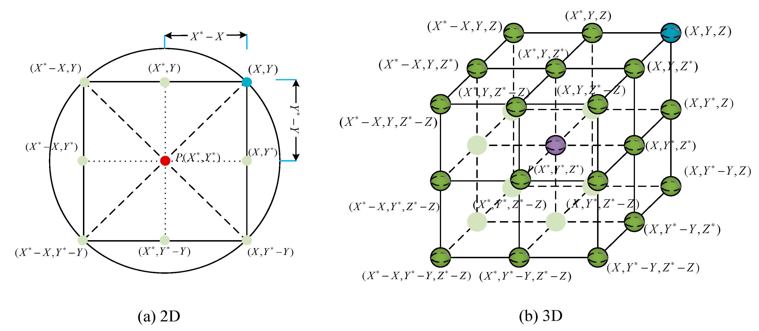
Figure 2a presents the basic principle of Equation (7) in solving 2D problems. The position of particles ( X , Y ) can be updated according to the position of the current optimal solution ( X * , Y * ) . By adjusting the coefficient vectors A and C, the development search can be implemented for different positions around the optimal solution according to the current position. Figure 2b shows the possible position of the particles after they are updated in 3D space. Due to the randomness of vectors A and C, the particles can reach any area among the key points in the search space. Therefore, the particles can be updated to an area near the optimal solution by using Equation (7) as a means of simulating the behavior of moving to the leading duck.
Step 2: If the new individual is worse than the old solution, select another particle P o p r a n d at random.
Step 3: If P o p r a n d is better than P o p i , the ith individual moves to the random particle P o p r a n d by Equation (11).
P o p i ( t + 1 ) = ( P o p r a n d ( t ) P o p i ( t ) ) × e l 2 + P o p i ( t ) ,
where l refers to the distance of the random particle and the ith individual.
Step 4: If P o p r a n d is equal to P o p i , it keeps unchanged.
Step 5: If P o p r a d is worse than P o p i , the random particle moves to the ith individual by Equation (11).
P o p r a n d ( t + 1 ) = ( P o p i ( t ) P o p r a n d ( t ) ) × e l 2 + P o p r a n d ( t ) ,

2.2.3. Flow of APO

Starting from the core of the swarm intelligence algorithm, global exploration and local development are carried out reasonably at the beginning to ensure a rapid convergence to a feasible solution. The operator uses random factors to ensure that the algorithm can move out of the local optimum. Moreover, the algorithm should have as few parameters as possible for simplification and ease in implementation. The anas platyrhynchos optimizer mainly consists of two operators, namely, the warning behavior and the moving process. These two operators ensure a balance between global exploration and local development. The pseudo code of the anas platyrhynchos optimizer is shown in Table 1.

3. Experiment and Application

To study our APO algorithm, experiments were carried out on both unconstrained and constrained global optimization problems. For unconstrained problems, 23 classic benchmark functions were employed. For constrained benchmark functions, the problem of multi-UAVs cooperative path planning were used. In addition, all the experiments in this section were performed on computer with 2.20 GHz Intel(R) Core(TM) i5-5200U processor and 8 GB of RAM using MATLAB 2016b.

3.1. Performance Analysis: Classic Benchmark Functions

To illustrate the relative success of APO on classic benchmark functions, a series of 23 widely used benchmarks selected from References [62,63,64,65,66,67] were introduced in this test. Table 2 and Table 3 present the detailed information about the different types of benchmarks. Our APO algorithm was compared with four well-known nature-based algorithms: GWO, WOA, PSO, and DE.
In this test, the population size N was set to 30. The maximum function evolution numbers (T) was set to 500. For each test function, 30 independent runs were carried out with random seeds. The parameter settings for the other compared algorithms in this test are detailed in Table 4. Such values represent the best parameter sets for these algorithms according to the original paper of GWO [8], WOA [9], PSO [2], and DE [68].
Table 5 summarizes the statistical results including mean, worst, best and SD of objective function values obtained by 30 independent runs for high-dimensional functions in Table 2. Compared with the other four algorithms, APO exhibited the best performance on the high-dimensional benchmark functions except function f4. Gray wolf optimization had a promising performance for optimizing f4, and APO exhibited the second-best performance on this function; meanwhile, APO sometimes has the best value for optimizing f4. From Table 5, it can be found that APO nearly finds all the best values of f9 and f11. According to the test results of Table 5, APO outperforms the other algorithms on high-dimensional benchmark functions.
The statistical results of the algorithms on low-dimensional benchmark functions are shown in Table 6. Compared with the other four algorithms, APO exhibited the best performance on f15, f21, f22 and f23. For f16 and f17, each algorithm nearly found all the best values. From Table 6, there is almost no difference in the performance on f18, f19 and f20 of each algorithm. In addition, although APO performs moderately on f14, it can also find the optimal value most of the time.
According to Table 5 and Table 6, the effectiveness of the APO algorithm can be verified. In very few test functions, the results of APO are slightly inferior to other swarm intelligence algorithms, but still meet the discussion of the no free lunch theorem. In 70% of the test functions, APO performs significantly better than other algorithms. In addition, in the 22% function, the APO result is not significantly different from other functions. Therefore, the performance of APO is obviously superior to other algorithms, and the APO has a higher priority in the choice of algorithm when solving optimization problems.
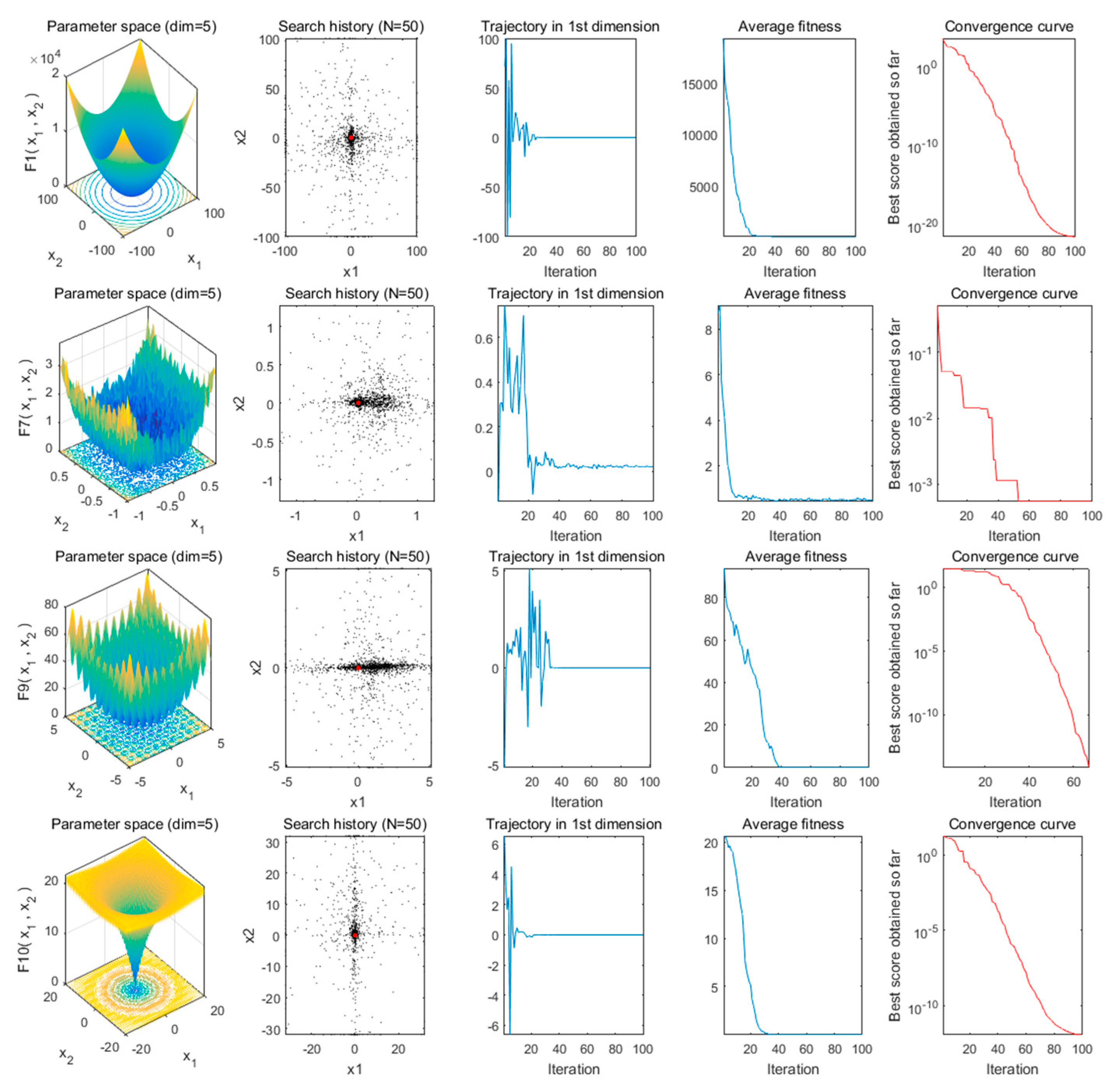
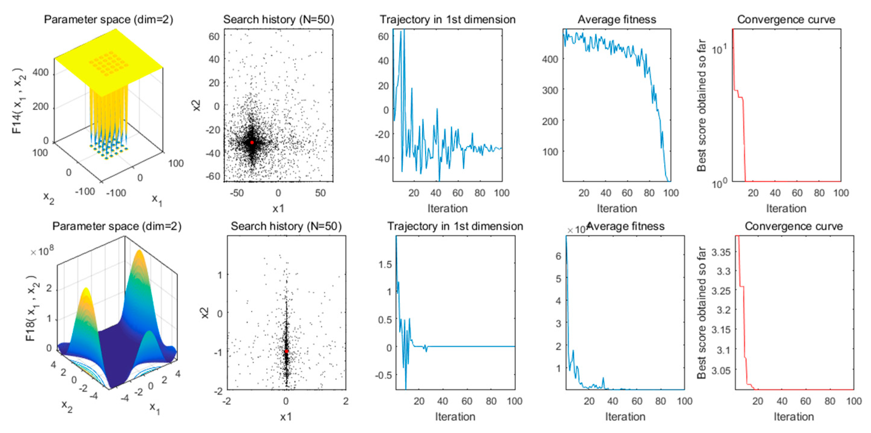
Berg [69] reported that mutation occurs during particle movement in the initial iteration process, and this mutation is conducive to the extensive and comprehensive exploration of particles in the search space. As the number of iterations increases, the mutation should be reduced accordingly to be able to fully demonstrate the local development ability of the algorithm. Column 3 in Figure 3 lists the search history and track of the first particle in the first dimension. Mutation occurs in the initial stage of the iteration. As the iteration continues, the mutation gradually decreases. According to Reference [69], this behavior ensures that the anas platyrhynchos optimizer eventually converges to a point in the search space. Meanwhile, Column 2 in Figure 3 shows the search history of the particles. The particles of the anas platyrhynchos optimizer tend to search for a prospective area in the search space to develop a better area. In this problem, we set the population number to 50 and the maximum number of iterations to 100 and used different dimensions from those in Table 2 and Table 3.
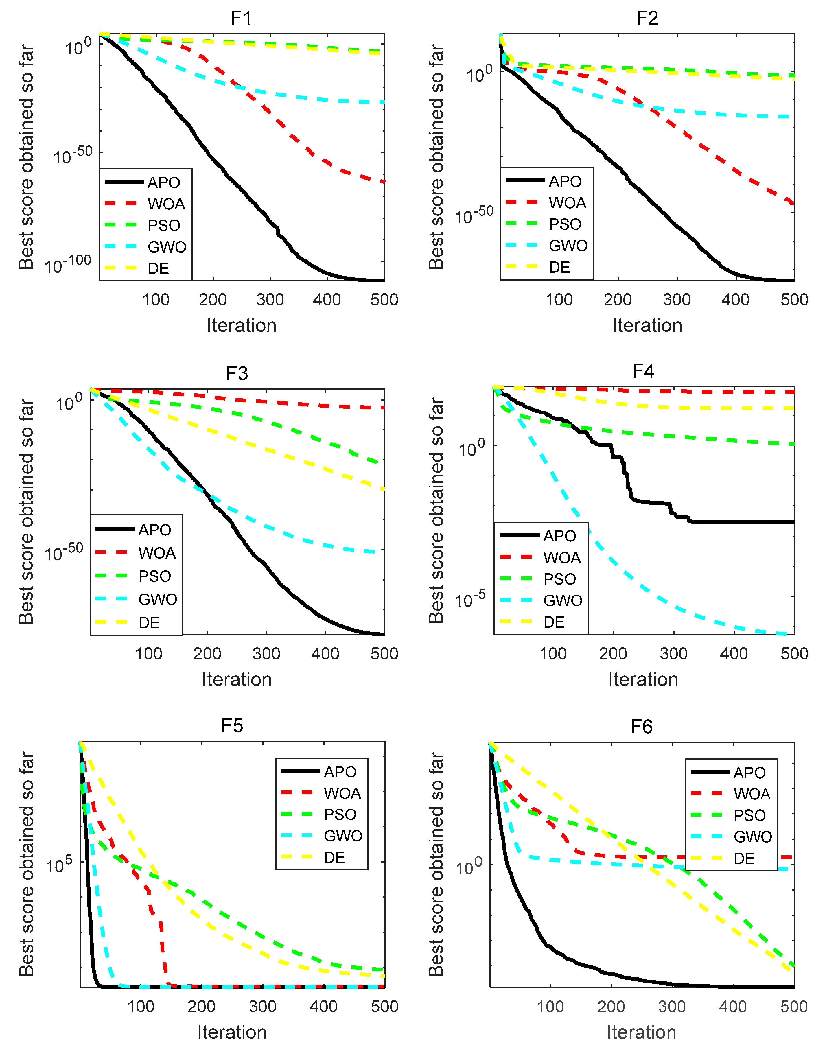
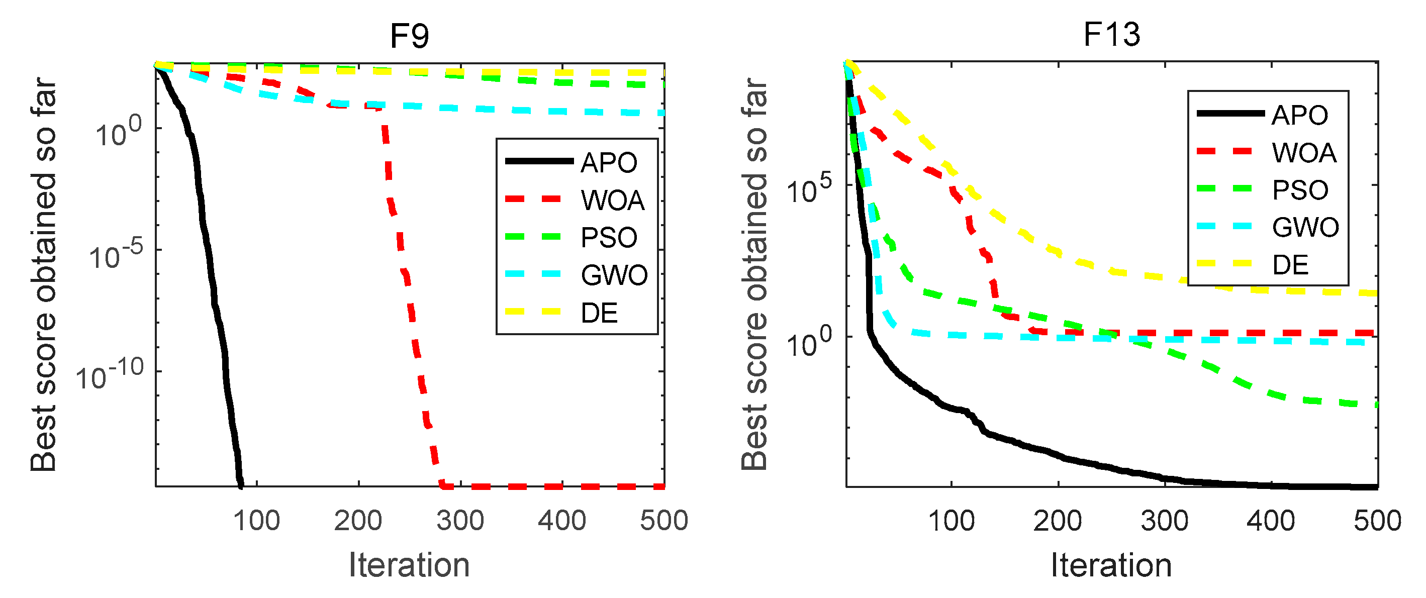
From a graphical point of view, Figure 4 and Figure 5 present the partly converged curves abstained by the five algorithms with 30 independent runs. When Figure 4 and Figure 5 are examined, APO converges rapidly for most test functions. Especially for the unimodal benchmark functions, APO has a faster convergence rate compared to the other algorithms. For the most multimodal functions, APO also presents the promising performance in convergence rate as shown in Figure 4 and Figure 5.
For detailed comparison, the Wilcoxon signed tanks test [70], in which Iman–Davenport’s procedure was used as a post-hoc procedure, was firstly used to make a pairwise comparison so as to illustrate the superiority of APO on the 23 test functions. The statistical results are summarized in Table 7. The p-values in Table 7 additionally present the superiority of the APO because most of the p-values are much smaller than 0.05.
In summary, the results of this section experimentally prove that the APO shows very competitive results and outperforms other well-known algorithms on the classic benchmark functions, and we state that the APO has merit among the other five algorithms. The next section inspects the performance of the APO in solving the problem of multi-UAVs cooperative path planning, and multi-UAVs cooperative path planning has high-dimension, multi-constraint, and space–time cooperation characteristics which are a challenging problem.

3.2. Engineering Application: Multi-UAVs Cooperative Path Planning

At present, the research methods used for path planning can be divided into the following categories: methods based on graph theory, methods based on potential field, search algorithms based on heuristic information, and algorithms based on swarm intelligence optimization. The results show that the swarm intelligence algorithm has obvious advantages in processing high-dimensional and multi-constraint challenges. The novel proposed APO can then be used to solve the problem on multi-UAVs cooperative path planning to further verify the algorithm’s effectiveness. In this part, we will cite the model in reference [71] and the algorithms involved to verify algorithm performance.

3.2.1. Modeling the UAV Cooperative Path Planning

In path planning, an appropriate planning space must be established in accordance with the flight environment and mission requirements. In the present work, taking a mountain background as a task environment, a digital elevation model is established using a random function to simulate peaks and other threat obstacles. The mountain model function is proposed in Reference [72]. This model consists of the original digital and threat equivalent terrain models. The former is expressed as:
z 1 ( x , y ) = sin ( y + a ) + b sin x + c cos ( d x 2 + y 2 ) + e cos y + f sin ( f x 2 + y 2 ) + g cos y
where x and y refer to the point coordinates on a horizontal projection plane; z 1 refers to the height coordinate that corresponds to the coordinate points on a horizontal plane; a, b, c, d, e, f, and g are the coefficients. The topography of a different landform can be obtained by changing parameters.
The threat equivalent terrain model is:
z 2 ( x , y ) = i = 1 k h ( i ) e x p ( ( x x 0 i x s i ) 2 ( y y o i y s i ) 2 ) ,
where z 2 refers to the height of the peak; h ( i ) refers to the height of the highest point of peak i on a base terrain; x 0 i and y 0 i refer to the coordinates of the highest point of peak i; x s i and y s i refer to the variables related to the slope of peak i along the x , y axis. If x s i and y s i are large, then the slope of the peak is flat and abrupt.
The final mountain threat model is obtained by integrating the original digital terrain model into the threat equivalent terrain model:
z ( x , y ) = m a x [ z 1 ( x , y ) , z 2 ( x , y ) ] ,
We set the starting point of a certain UAV as S ( x 0 , y 0 , z 0 ) and the target point as E ( x e , y e , z e ) . The number of waypoints is n, and the waypoints searched can be represented by { S , P 1 , P 2 , , P n , E } ; among these variables, the coordinate of a track node is P = ( x p , y p , z p ) .

3.2.2. Path Cost Function

The purpose of multi-UAV cooperative path planning is that, on the premise of satisfying the requirements of a safe flight and space–time cooperation, every UAV can search the corresponding path, and the synthetic path cost of UAV fleet must be the least. Therefore, path planning requires the establishment of a path cost function as an index to evaluate the quality of a path. The satisfaction of the spatial and temporal cooperative constraints of multi-UAV by considering the dynamics and threat constraints of a single UAV in multi-UAV cooperative path planning is required. Thus, given the planning objective, the following cost indexes are considered in the present work: the performance indexes of a single UAV include fuel consumption, maximum climb/slide angle, flying altitude, peak threat, and multi-UAV time cooperation. Spatial cooperation is manifested in multi-UAV path collision avoidance. We set different flight altitudes that must be avoided by each UAV. The synthetic cost function is established as:
J = ω 1 J f u e l + ω 2 J a n g l e + ω 3 J h e i g h t + ω 4 J t h r e a t + ω 5 J c o o p ,
where ω 1 , ω 2 , ω 3 , ω 4 and ω 5 refer to the weights of different cost indexes, and the sum of weights is 1. The paths that satisfy different requirements can be obtained by adjusting the weights. To ensure that all cost indexes are involved in path planning, the functions are normalized in accordance with the range of their values, and then weighted summation is performed.
Fuel consumption cost is related to the length of flight path and flying speed. Assuming that UAVs consistently fly at a certain speed, fuel costs can be replaced by the length of the path:
J f u e l = i = 1 n 1 ( x i + 1 x i ) 2 + ( y i + 1 + y i ) 2 + ( z i + 1 z i ) 2 ,
where ( x i + 1 , y i + 1 , z i + 1 ) and ( x i , y i , z i ) correspond to the coordinates of the adjacent path points.
J a n g l e refers to the cost of the maximum climb/slide angle and is expressed as:
J a n g l e = i = 1 n θ i | θ i = a r c t a n ( | z i + 1 z i | ( x i + 1 x i ) 2 + ( y i + 1 y i ) 2 ) ,
where θ i refers to the climb/slide angle of the adjacent points of a certain path.
To satisfy the requirements of flight safety and concealment, the flight altitude cannot be overly low or high. Height cost can be expressed as:
J h e i g h t = i = 1 n | h i s a f t h i | ,
where h i refers to the height of path point i on a certain path, and s a f t h i refers to the minimum safety height for each UAV.
Collision with the mountain in the flying course of the UAV must be avoided. In Reference [73], the peak model is represented by a cone approximate representation. The path is divided into m equal sections, and m−1 sampling points are obtained in the center. The threat cost of the whole path is expressed as
J t h r e a t = i = 1 n j = 1 m k = 1 K t h r e a t ( j , k ) ,
where n refers to the number of path points, K represents the number of peaks, and t h r e a t ( j , k ) is the threat cost of the sampling point ( x i , y i , z i ) in the current section and a certain peak and is expressed as:
t h r e a t ( j , k ) = { 0 h j > H ( k )   o r   d T > R T + d m i n R T ( h ) + d T m i n d T h j < H ( k )   a n d   d T < R T + d T m i n R T ( h ) = ( H ( k ) h ) / tan θ
where n refers to the number of path points, K represents the number of peaks, H(k) refers to the height of peak k, and R T refers to the maximum extension radius. Moreover, h j is the flying altitude of the current UAV, d T refers to the distance from the UAV to the symmetrical axis of the peak, d T m i n denotes the minimum distance allowed on the terrain, and θ refers to the slope of the terrain. The terrain threat is depicted in Figure 6.
Cooperative cost function implies time cooperation. All UAVs are required to reach the target point simultaneously as far as possible. If the course of a certain path cannot satisfy the time cooperative constraints, then the path must be corrected. Assuming that the flying speed of the UAV is in the range of [ υ m i n , υ m a x ] and the course of the UAV i is L i , its flight time period is T i [ T m i n i , T m a x i ] . Similarly, assuming that the flying time of UAV j is in the range of T j [ T m i n j , T m a x j ] , if the flight time of the two UAVs intersects, then temporal cooperation is feasible, that is
T i n t e r = T i T j ,
in accordance with the temporal cooperation evaluation formula between paths in Reference [74], the temporal cooperation cost function is obtained on the basis of the planning model in the present work:
J c o o p T = { 1 T i n t e r = 2 0 < T i n t e r < r a n d × T m i n 3 T i n t e r T m i n T i n t e r > 1 3 T m i n
where T m i n refers to a time period with a small range of a certain path in the flight time period, and T i n t e r represents the intersection of the flight time for two paths.

3.2.3. Multi-Population Track Coding

The idea of multi-population is combined in this work to construct the multi-UAVs track set. When the algorithm is adopted to perform a search, the number of populations is determined in accordance with the number of UAVs, and the process of UAV searching path is mapped to the updating process of the population. The position of the anas platyrhynchos in each sub-population corresponds to a flying path of the mapped UAV. The optimal solution in the sub-population corresponds to the optimal path of this UAV. The optimal solution of all sub-populations corresponds to the cooperative path of UAVs.
If all UAVs on a mission are set as U = { U i , i = 1 , 2 , , N u } , then the corresponding number of anas platyrhynchos population is N u . The number of anas platyrhynchos individuals in each sub-population is set as m , and the anas platyrhynchos individuals in the sub-population can be represented as X = { X i , i = 1 , 2 , , m } . The position of anas platyrhynchos i in the search space is X i = { X i 1 , X i 2 , , X i n } , which represents the midway point of a path in addition to the starting and the target points. The coordinate of each path point is X n = { x i n , y i n , z i n } . The fitness value of the anas platyrhynchos individual corresponds to the cost function value of a certain path. If the fitness is favorable, then the path is optimal. In the process of searching and comparing the fitness values of individuals in the population, the anas platyrhynchos individuals at the favorable position are obtained as the leading duck. The algorithm is guided to search continuously in the direction with small fitness values, thereby resulting in many cooperative paths.
When the APO algorithm is initialized, a group of anas platyrhynchos is randomly generated in the region of search. When an individual’s three-dimensional position coordinates are randomly generated, the computational load is large, and the search efficiency is low. Therefore, in this work, an equal division was performed for the coordinates of individuals in the direction of the x-axis based on the number of the waypoints set at initialization. In the searching process, the positions in the y- and z-axes were updated. Boundary control was performed when the position was updated. The planning problem was transformed into a search optimization problem in a two-dimensional space.
Based on the APO algorithm in this work, the specific flow of the multi-UAVs cooperative path planning is exhibited in Figure 7.

3.2.4. Simulation Validation

The planning space was set as 100 km × 100 km × 500 m, including six peaks. The parameters of the original digital terrain model were set to a = 0.1, b = 0.01, c = 1, d = 0.1, e = 0.2, f = 0.4, and g = 0.02. The height of the peak, horizontal coordinates of the highest point, and slope parameters are listed in Table 8. Multi-UAV cooperative path planning was conducted under a known mission assignment scheme. In the simulation experiment, the path sub-population was initialized in accordance with the number of UAVs. The numbers of individuals in the sub-population, iterations, and path points were 50, 100, and 10, respectively. The weight coefficients of all cost functions corresponded to 0.4, 0.2, 0.1, 0.2, and 0.1. The flight speed range of the UAV was 40–60 m/s.
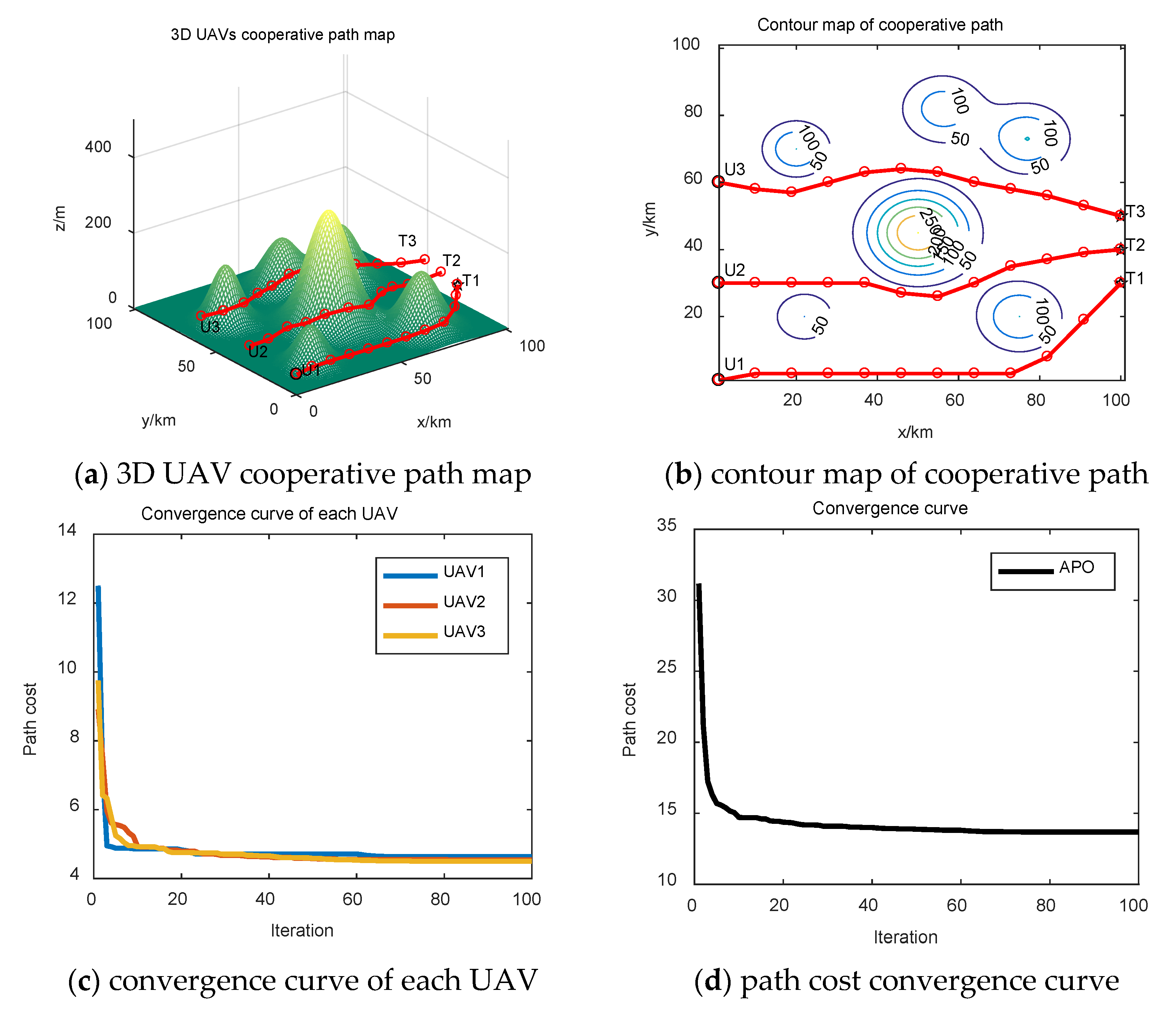
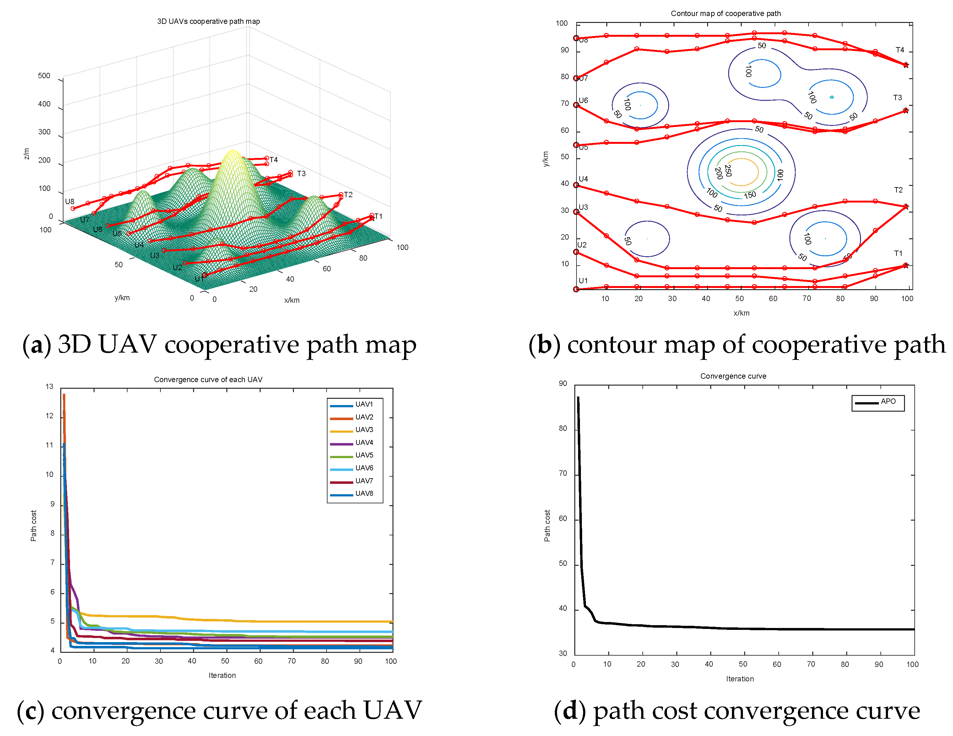
Case 1: Three UAVs begin from the starting point and arrived at the designated target point to perform tasks. The coordinates of the starting and target points are presented in Table 9.
The three-dimensional path planning and contour map of each UAV are displayed in Figure 8a,b. The cost and synthetic path cost convergence curves of each UAV are plotted in Figure 8c,d. Figure 8 illustrates that all UAVs could effectively avoid the threat and reach the target point. The cost function values of each UAV gradually converge with the increase in iteration times, thereby verifying the effectiveness of the algorithm. Through a simulation, the flight time intervals (unit: s) and range (unit: km) of each UAV are presented in Table 10. The time intersection is [1849.0089, 2554.5307]. The time synergy requirement can be satisfied by setting different flight speeds for all UAVs.
Case 2: Four UAVs fly to two target points. The coordinates of the starting and the target points are listed in Table 11.
The planned path diagrams of UAVs are obtained as depicted in Figure 9a,b. The path cost convergence and synthetic cost curves of each UAV are plotted in Figure 9c,d. Through a simulation, the flight time intervals (unit: s) and range (unit: km) of each UAV are presented in Table 12. The time intersection is [1961.975, 2417.0379]. The planned paths and voyages are close and can effectively avoid obstacles. If the UAVs are close to one another, then collisions can be avoided by setting different flight altitudes.
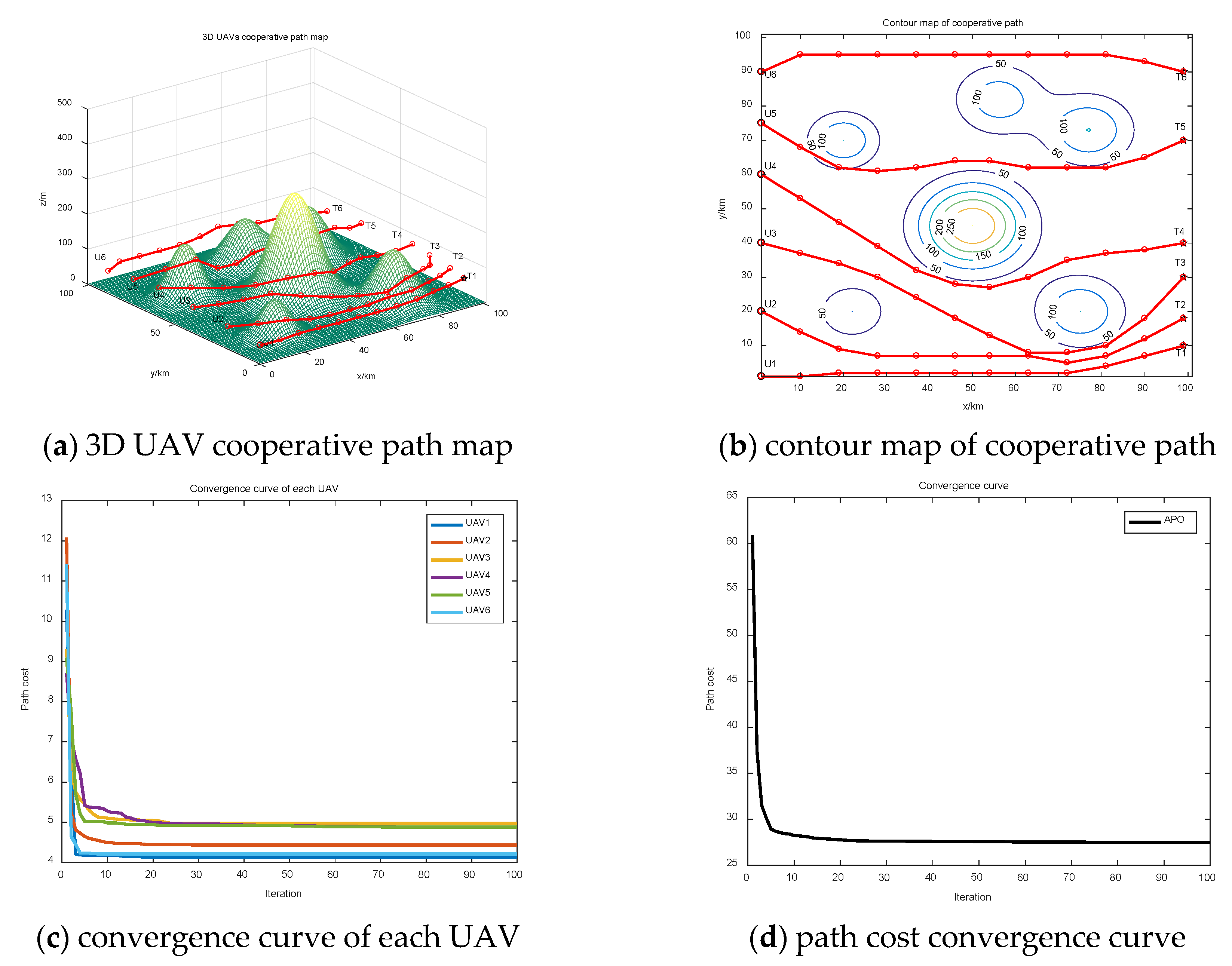
Case 3: Six UAVs fly to six target points. The coordinates of the starting and the target points are listed in Table 13.
The result of case 3 was obtained as depicted in Figure 10. Through a simulation, the flight time intervals (unit: s) and range (unit: km) of each UAV are presented in Table 14. The time intersection is [1924.111, 2481.215]. The planned paths and voyages are close and can effectively avoid obstacles.
Case 4: Eight UAVs fly to four target points. The coordinates of the starting and the target points are listed in Table 15.
The result of case 4 was obtained as depicted in Figure 11. Through a simulation, the flight time intervals (unit: s) and range (unit: km) of each UAV are presented in Table 16. The time intersection is [1922.8382, 2493.2072]. The planned paths and voyages are close and can effectively avoid obstacles.
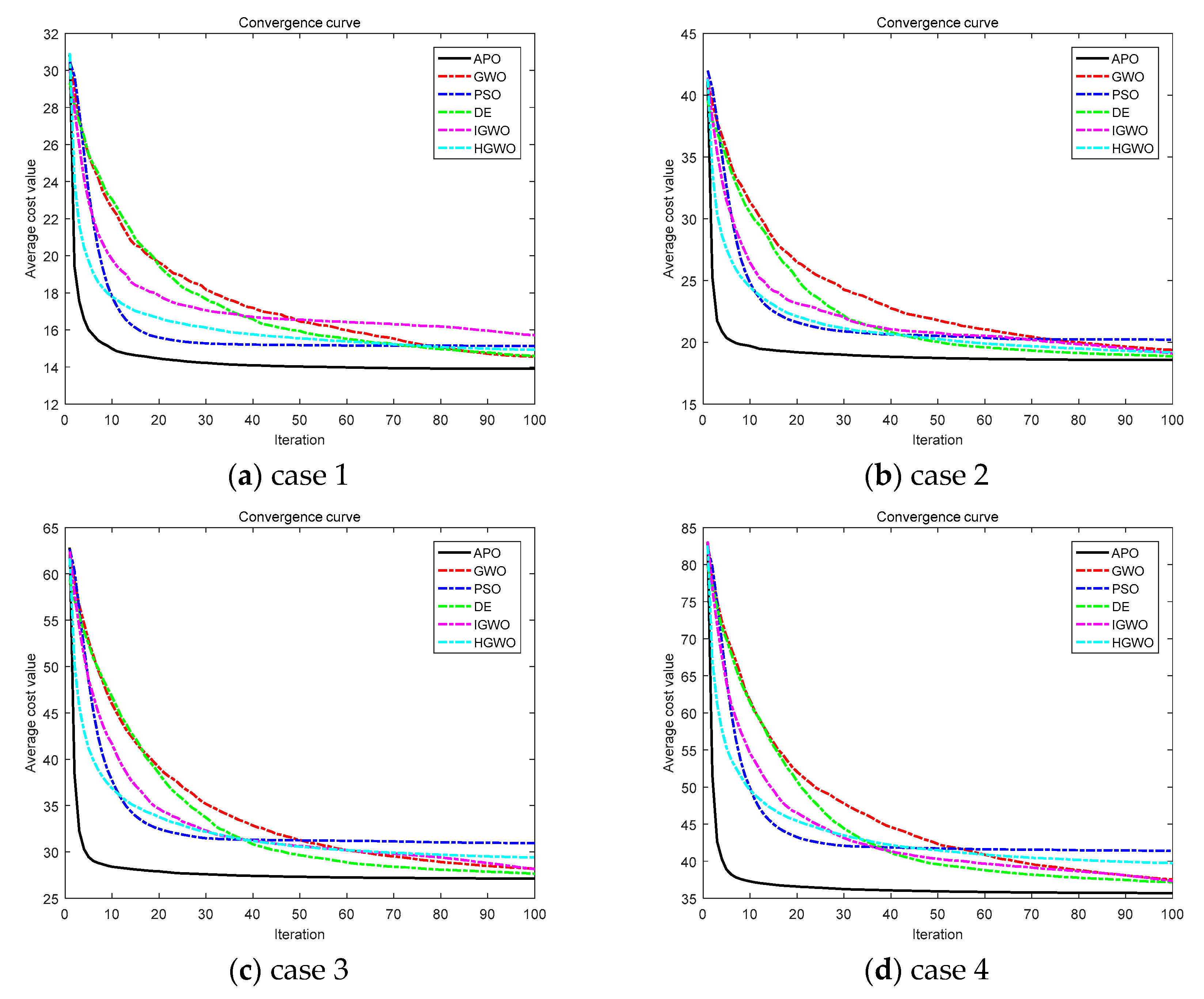
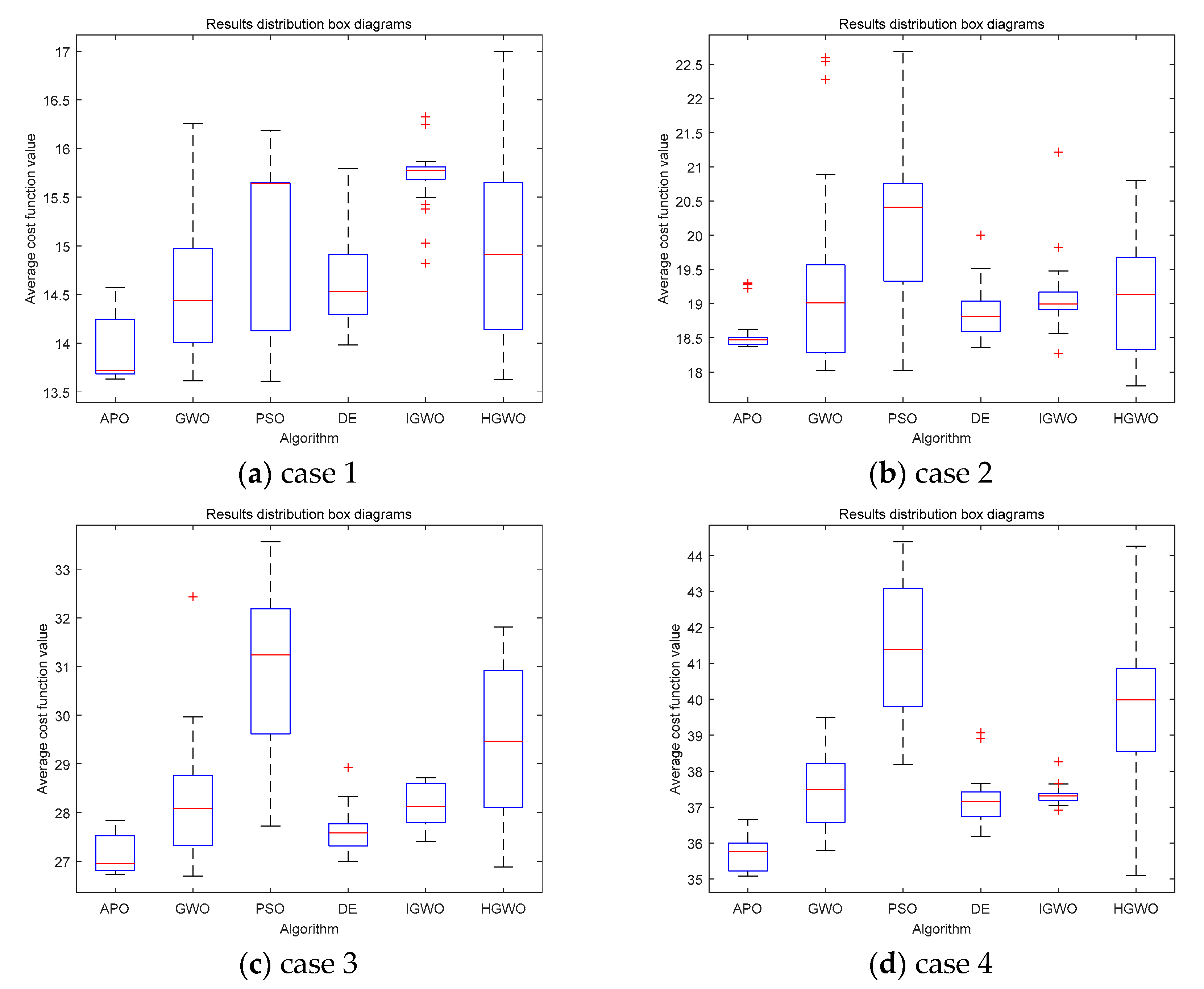
The performance of the anas platyrhynchos optimizer is further verified in this work. In particular, the PSO, DE, and GWO algorithms, the improved GWO based on chaos thought (HGWO) [71], and the improved GWO with dynamic weighted average combined with the static average method (IGWO) [50] are used to implement multi-cooperative path planning in different cases. The simulation result was subsequently compared with the algorithms in this study to further verify the effectiveness of the novel algorithm. Each algorithm was run 30 times to avoid the influence of randomness, with the number of populations set to 50 and the number of iterations set to 100. Fair comparison was ensured by setting the same evaluation approach for all common parameters such as the population size, dimension, and maximum iteration of the different algorithms. The relevant parameters of these algorithms are shown in Table 17. Such values represent the best parameter sets for these algorithms according to the original paper of GWO [8], HGWO [71], IGWO [50], PSO [2], and DE [68]. The convergence curve of the 3D-integrated path cost of each case is shown in Figure 12, and the distribution of the operation results (30 times of testing) is shown in Figure 13. The average time of each algorithm in each scenario are shown in Table 18.
The results show that the cost functions of each algorithm can converge to a certain value, which meets the actual requirements of planning. As can be seen from Figure 11, the final convergence value of APO in each case was smaller than other algorithms, and the convergence speed was also faster. The comparison shows that the convergence speed and the convergence accuracy of the method proposed in this study was faster than those of the other algorithms. In addition, it can be seen from Table 17 that the calculation time of APO was better than other algorithms in case 1, 2, and 4. In case 3, APO was only 0.25 s worse than the best performing GWO. Thus, APO’s advantage in computing time was verified. The results of multiple runs in various scenarios in Figure 12 show that APO can find a better solution than other algorithms in multiple runs, and then verifies the stability of the algorithm.
In summary, the APO algorithm solves the problems of slow convergence speed and low convergence accuracy of other algorithms. The calculation time is obviously better than other algorithms, and it has good stability. Therefore, the APO was superior in solving the problem of multi-UAVs cooperative path planning. Furthermore, the successful application of APO algorithm in the path planning problem provides new ideas for other practical engineering problems.

4. Conclusions

Inspired by the cluster action of anas platyrhynchos, a novel type of swarm intelligence algorithm referred as the anas platyrhynchos optimizer was proposed in this study. The global optimization function problems and multi-UAVs cooperative path planning engineering problems were solved using this algorithm. The performance of APO was analyzed using 23 classical benchmark function. The comparative experiment with the PSO, DE, WOA, and GWO algorithms verified the superiority of the anas platyrhynchos optimizer. Moreover, the anas platyrhynchos optimizer was applied to multi-UAV cooperative path planning with high-dimension, multi-constraint, time–space cooperation characteristics to further verify the algorithm’s effectiveness. The multi-UAV cooperative path planning model was first constructed. Four challenging flight scenarios were set-up. Then, the multi-UAV cooperative path planning problems were solved using the anas platyrhynchos optimizer in four flight scenarios. The digital simulation experiment was carried out using MATLAB. The simulation result was further compared with the results from using the PSO, DE, GWO, IGWO, and HGWO algorithms. The final results indicate that the anas platyrhynchos optimizer was better than the other algorithms in terms of convergence speed, operation time, and calculation accuracy.
The current research mainly focuses on the anas platyrhynchos optimizer and its application in solving multi-UAV cooperative path planning problems. In the future, we intend to apply the anas platyrhynchos optimizer to more practical engineering problems and examine further the performance of this algorithm in terms of task allocation, image detection, pattern recognition, and other practical engineering problems. We also intend to develop much more complicated problems and enhance the solutions by using the anas platyrhynchos optimizer.

Author Contributions

Conceptualization, Y.Z., P.W., Y.L. (Yanbin Liu) and X.Z.; Data curation, P.W.; Formal analysis, Y.Z. and P.W.; Funding acquisition, Y.Z. and L.Y.; Investigation, Y.Z. and P.W.; Methodology, Y.Z. and P.W.; Project administration, Y.Z. and L.Y.; Resources, P.W.; Supervision, Y.Z., L.Y. and Y.L. (Yuping Lu); Validation, P.W.; Visualization, P.W.; Writing—original draft, P.W.; Writing—review and editing, Y.Z. and P.W. All authors have read and agreed to the published version of the manuscript.

Funding

This research was funded by the Six Talent Peaks Project in Jiangsu Province of China (KTHY-025).

Conflicts of Interest

The authors declare no conflict of interest.

References

  1. Branke, J.; Guntsch, M. Solving the probabilistic TSP with ant colony optimization. J. Math. Model. Algorithms 2004, 3, 403–425. [Google Scholar] [CrossRef]
  2. Poli, R.; Kennedy, J.; Blackwell, T. Particle swarm optimization. Swarm Intell. 2007, 1, 33–57. [Google Scholar] [CrossRef]
  3. Dorigo, M.; Birattari, M.; Stutzle, T. Ant colony optimization. IEEE Comput. Intell. Mag. 2006, 1, 28–39. [Google Scholar] [CrossRef]
  4. Yang, X.S.; Gandomi, A.H. Bat algorithm: A novel approach for global engineering optimization. Eng. Comput. 2012, 29, 1–18. [Google Scholar] [CrossRef] [Green Version]
  5. Mirjalili, S. Dragonfly algorithm: A new meta-heuristic optimization technique for solving single-objective, discrete, and multi-objective problems. Neural Comput. Appl. 2016, 27, 1053–1073. [Google Scholar] [CrossRef]
  6. Mirjalili, S.Z.; Mirjalili, S.; Saremi, S.; Faris, H.; Aljarah, I. Grasshopper optimization algorithm for multi-objective optimization problems. Appl. Intell. 2018, 48, 805–820. [Google Scholar] [CrossRef]
  7. Mirjalili, S. Moth-flame optimization algorithm: A novel nature-inspired heuristic paradigm. Knowl. Based Syst. 2015, 89, 228–249. [Google Scholar] [CrossRef]
  8. Mirjalili, S.; Mirjalili, S.M.; Lewis, A. Grey wolf optimizer. Adv. Eng. Softw. 2014, 69, 46–61. [Google Scholar] [CrossRef] [Green Version]
  9. Mirjalili, S.; Lewis, A. The whale optimization algorithm. Adv. Eng. Softw. 2016, 95, 51–67. [Google Scholar] [CrossRef]
  10. Chen, Y.; Vepa, R.; Shaheed, M.H. Enhanced and speedy energy extraction from a scaled-up pressure retarded osmosis process with a whale optimization based maximum power point tracking. Energy 2018, 153, 618–627. [Google Scholar] [CrossRef]
  11. Saha, A.; Saikia, L.C. Performance analysis of combination of ultra-capacitor and superconducting magnetic energy storage in a thermal-gas AGC system with utilization of whale optimization algorithm optimized cascade controller. J. Renew. Sustain. Energy 2018, 10, 014103. [Google Scholar] [CrossRef]
  12. Jadhav, A.R.; Shankar, T. Whale optimization based energy-efficient cluster head selection algorithm for wireless sensor networks. arXiv 2017, arXiv:1711.09389. [Google Scholar]
  13. Kumawat, I.R.; Nanda, S.J.; Maddila, R.K. Positioning LED panel for uniform illuminance in indoor VLC system using whale optimization. In Optical and Wireless Technologies; Springer: Berlin/Heidelberg, Germany, 2018; pp. 131–139. [Google Scholar]
  14. Sreenu, K.; Sreelatha, M. W-Scheduler: Whale optimization for task scheduling in cloud computing. Clust. Comput. 2019, 22, 1087–1098. [Google Scholar] [CrossRef]
  15. Mousavirad, S.J.; Ebrahimpour-Komleh, H. Multilevel image thresholding using entropy of histogram and recently developed population-based metaheuristic algorithms. Evol. Intell. 2017, 10, 45–75. [Google Scholar] [CrossRef]
  16. Hassan, G.; Hassanien, A.E. Retinal fundus vasculature multilevel segmentation using whale optimization algorithm. Signal Image Video Process 2018, 12, 263–270. [Google Scholar] [CrossRef]
  17. Yuan, P.; Guo, C.; Zheng, Q.; Ding, J. Sidelobe suppression with constraint for MIMO radar via chaotic whale optimisation. Electron. Lett. 2018, 54, 311–313. [Google Scholar] [CrossRef]
  18. Pathak, V.K.; Singh, A.K. Accuracy control of contactless laser sensor system using whale optimization algorithm and moth-flame optimization. TM-Tech. Mess. 2017, 84, 734–746. [Google Scholar] [CrossRef]
  19. Zhang, C.; Fu, X.; Ligthart, L.P.; Peng, S.; Xie, M. Synthesis of broadside linear aperiodic arrays with sidelobe suppression and null steering using whale optimization algorithm. IEEE Antennas Wirel. Propag. Lett. 2018, 17, 347–350. [Google Scholar] [CrossRef]
  20. Hegazy, A.E.; Makhlouf, M.A.; El-Tawel, G.S. Dimensionality reduction using an improved whale optimization algorithm for data classification. Int. J. Mod. Educ. Comput. Sci. 2018, 11, 37. [Google Scholar] [CrossRef] [Green Version]
  21. Zamani, H.; Nadimi-Shahraki, M.H. Feature selection based on whale optimization algorithm for diseases diagnosis. Int. J. Comput. Sci. Inf. Secur. 2016, 14, 1243. [Google Scholar]
  22. Mafarja, M.; Mirjalili, S. Whale optimization approaches for wrapper feature selection. Appl. Soft Comput. 2018, 62, 441–453. [Google Scholar] [CrossRef]
  23. Yu, Y.; Wang, H.; Li, N. Automatic carrier landing system based on active disturbance rejection control with a novel parameters optimizer. Aerosp. Sci. Technol. 2017, 69, 149–160. [Google Scholar] [CrossRef]
  24. Wu, J.; Wang, H.; Li, N. Path planning for solar-powered UAV in urban environment. Neurocomputing 2018, 275, 2055–2065. [Google Scholar] [CrossRef]
  25. Kaveh, A.; Ghazaan, M.I. Enhanced whale optimization algorithm for sizing optimization of skeletal structures. Mech. Based Des. Struct. Mach. 2017, 45, 345–362. [Google Scholar] [CrossRef]
  26. Kaveh, A. Sizing optimization of skeletal structures using the enhanced whale optimization algorithm. In Applications of Metaheuristic Optimization Algorithms in Civil Engineering; Springer: Berlin/Heidelberg, Germany, 2017; pp. 47–69. [Google Scholar]
  27. Wu, J.; Wang, H.; Li, N. Distributed trajectory optimization for multiple solar-powered UAVs target tracking in urban environment by Adaptive Grasshopper Optimization Algorithm. Aerosp. Sci. Technol. 2017, 70, 497–510. [Google Scholar] [CrossRef]
  28. Barman, M.; Choudhury, N.B.D.; Sutradhar, S. A regional hybrid GOA-SVM model based on similar day approach for short-term load forecasting in Assam, India. Energy 2018, 145, 710–720. [Google Scholar] [CrossRef]
  29. El-Fergany, A.A. Electrical characterisation of proton exchange membrane fuel cells stack using grasshopper optimiser. IET Renew. Power Gener. 2017, 12, 9–17. [Google Scholar] [CrossRef]
  30. Łukasik, S.; Kowalski, P.A.; Charytanowicz, M. Data clustering with grasshopper optimization algorithm. In Proceedings of the 2017 Federated Conference on Computer Science and Information Systems (FedCSIS), Prague, Czech Republic, 3–6 September 2017; pp. 71–74. [Google Scholar]
  31. Rajput, N.; Chaudhary, V.; Dubey, H.M. Optimal generation scheduling of thermal System using biologically inspired grasshopper algorithm. In Proceedings of the 2017 2nd International Conference on Telecommunication and Networks (TEL-NET), Noida, India, 10–11 August 2017; pp. 1–6. [Google Scholar]
  32. Zhang, X.; Miao, Q.; Zhang, H. A parameter-adaptive VMD method based on grasshopper optimization algorithm to analyze vibration signals from rotating machinery. Mech. Syst. Signal Process. 2018, 108, 58–72. [Google Scholar] [CrossRef]
  33. Zhao, H.; Zhao, H.; Guo, S. Short-term wind electric power forecasting using a novel multi-stage intelligent algorithm. Sustainability 2018, 10, 881. [Google Scholar] [CrossRef] [Green Version]
  34. Ahanch, M.; Asasi, M.S.; Amiri, M.S. A Grasshopper Optimization Algorithm to solve optimal distribution system reconfiguration and distributed generation placement problem. In Proceedings of the 2017 IEEE 4th International Conference on Knowledge-Based Engineering and Innovation (KBEI), Tehran, Iran, 22 December 2017; IEEE: Piscataway, NJ, USA, 2017; pp. 659–666. [Google Scholar]
  35. Ibrahim, H.T.; Mazher, W.J.; Ucan, O.N. A grasshopper optimizer approach for feature selection and optimizing SVM parameters utilizing real biomedical data sets. Neural Comput. Appl. 2019, 31, 5965–5974. [Google Scholar] [CrossRef]
  36. Amaireh, A.A.; Alzoubi, A.; Dib, N.I. Design of linear antenna arrays using antlion and grasshopper optimization algorithms. In Proceedings of the 2017 IEEE Jordan Conference on Applied Electrical Engineering and Computing Technologies (AEECT), Aqaba, Jordan, 11–13 October 2017; IEEE: Piscataway, NJ, USA, 2017; pp. 1–6. [Google Scholar]
  37. Hamad, A.; Houssein, E.H.; Hassanien, A.E. Hybrid grasshopper optimization algorithm and support vector machines for automatic seizure detection in EEG signals. In International Conference on Advanced Machine Learning Technologies and Applications; Springer: Berlin/Heidelberg, Germany, 2018; pp. 82–91. [Google Scholar]
  38. Hekimoğlu, B.; Ekinci, S. Grasshopper optimization algorithm for automatic voltage regulator system. In Proceedings of the 2018 5th International Conference on Electrical and Electronic Engineering (ICEEE), Istanbul, Turkey, 3–5 May 2018; IEEE: Piscataway, NJ, USA, 2018; pp. 152–156. [Google Scholar]
  39. Heidari, A.A.; Faris, H.; Aljarah, I. An efficient hybrid multilayer perceptron neural network with grasshopper optimization. Soft Comput. 2019, 23, 7941–7958. [Google Scholar] [CrossRef]
  40. Faris, H.; Aljarah, I.; Mirjalili, S. Evolving radial basis function networks using moth–flame optimizer[M]. In Handbook of Neural Computation; Academic Press: Cambridge, MA, USA, 2017; pp. 537–550. [Google Scholar]
  41. Hassanin, M.F.; Shoeb, A.M.; Hassanien, A.E. Designing multilayer feedforward neural networks using multi-verse optimizer. In Handbook of Research on Machine Learning Innovations and Trends; IGI Global: Hershey, PA, USA, 2017; pp. 1076–1093. [Google Scholar]
  42. Benmessahel, I.; Xie, K.; Chellal, M. A new evolutionary neural networks based on intrusion detection systems using multiverse optimization. Appl. Intell. 2018, 48, 2315–2327. [Google Scholar] [CrossRef]
  43. Faris, H.; Hassonah, M.A.; Ala’M, A.Z. A multi-verse optimizer approach for feature selection and optimizing SVM parameters based on a robust system architecture. Neural Comput. Appl. 2018, 30, 2355–2369. [Google Scholar] [CrossRef]
  44. Rosenberg, A.; Hirschberg, J. V-measure, A conditional entropy-based external cluster evaluation measure. In Proceedings of the 2007 Joint Conference on Empirical Methods in Natural Language Processing and Computational Natural Language Learning (EMNLP-CoNLL), Prague, Czech Republic, 28–30 June 2007; Association for Computational Linguistics: Stroudsburg, PA, USA, 2007; pp. 410–420. [Google Scholar]
  45. Wolpert, D.H.; Macready, W.G. No free lunch theorems for optimization. IEEE Trans. Evol. Comput. 1997, 1, 67–82. [Google Scholar] [CrossRef] [Green Version]
  46. Emary, E.; Zawbaa, H.M.; Hassanien, A.E. Binary grey wolf optimization approaches for feature selection. Neurocomputing 2016, 172, 371–381. [Google Scholar] [CrossRef]
  47. Panwar, L.K.; Reddy, S.; Verma, A. Binary grey wolf optimizer for large scale unit commitment problem. Swarm Evol. Comput. 2018, 38, 251–266. [Google Scholar] [CrossRef]
  48. Jayabarathi, T.; Raghunathan, T.; Adarsh, B.R. Economic dispatch using hybrid grey wolf optimizer. Energy 2016, 111, 630–641. [Google Scholar] [CrossRef]
  49. Srikanth, K.; Panwar, L.K.; Panigrahi, B.K. Meta-heuristic framework, Quantum inspired binary grey wolf optimizer for unit commitment problem. Comput. Electr. Eng. 2018, 70, 243–260. [Google Scholar] [CrossRef]
  50. Liu, C.A.; Wang, X.P.; Liu, C.Y.; Wu, H. Three-dimensional route planning for unmanned aerial vehicle based on improved grey wolf optimizer. J. Huazhong Univ. Sci. Technol. 2017, 45, 38–42. [Google Scholar]
  51. Singh, N.; Singh, S.B. Hybrid algorithm of particle swarm optimization and grey wolf optimizer for improving convergence performance. J. Appl. Math. 2017, 2030489. [Google Scholar] [CrossRef]
  52. Ab Rashid, M.F.F. A hybrid Ant-Wolf Algorithm to optimize assembly sequence planning problem. Assem. Autom. 2017, 37, 238–248. [Google Scholar] [CrossRef] [Green Version]
  53. ElGayyar, M.; Emary, E.; Sweilam, N.H. A hybrid Grey Wolf-bat algorithm for global optimization. In International Conference on Advanced Machine Learning Technologies and Applications; Springer: Berlin/Heidelberg, Germany, 2018; pp. 3–12. [Google Scholar]
  54. Pan, J.S.; Dao, T.K.; Chu, S.C. A novel hybrid GWO-FPA algorithm for optimization applications. In International Conference on Smart Vehicular Technology, Transportation, Communication and Applications; Springer: Berlin/Heidelberg, Germany, 2017; pp. 274–281. [Google Scholar]
  55. Debnath, M.K.; Mallick, R.K.; Sahu, B.K. Application of hybrid differential evolution–grey wolf optimization algorithm for automatic generation control of a multi-source interconnected power system using optimal fuzzy–PID controller. Electr. Power Compon. Syst. 2017, 45, 2104–2117. [Google Scholar] [CrossRef]
  56. Singh, N.; Singh, S.B. A novel hybrid GWO-SCA approach for optimization problems. Eng. Sci. Technol. Int. J. 2017, 20, 1586–1601. [Google Scholar] [CrossRef]
  57. Zhang, X.; Kang, Q.; Cheng, J.; Wang, X. A novel hybrid algorithm based on biogeography-based optimization and grey wolf optimizer. Appl. Soft Comput. 2018, 67, 197–214. [Google Scholar] [CrossRef]
  58. Trivedi, I.N.; Jangir, P.; Kumar, A. A novel hybrid PSO–WOA algorithm for global numerical functions optimization. In Advances in Computer and Computational Sciences; Springer: Berlin/Heidelberg, Germany, 2018; pp. 53–60. [Google Scholar]
  59. Kaveh, A.; Rastegar Moghaddam, M. A hybrid WOA-CBO algorithm for construction site layout planning problem. Sci. Iran. 2018, 25, 1094–1104. [Google Scholar] [CrossRef] [Green Version]
  60. Yang, X.S.; Deb, S. Cuckoo search via Lévy flights. In Proceedings of the 2009 World Congress on Nature & Biologically Inspired Computing (NaBIC), Coimbatore, India, 9–11 December 2009; IEEE: Piscataway, NJ, USA, 2009; pp. 210–214. [Google Scholar]
  61. Zelinka, I. SOMA—Self-Organizing Migrating Algorithm. In New Optimization Techniques in Engineering; Springer: Berlin/Heidelberg, Germany, 2004; pp. 167–217. [Google Scholar]
  62. Yao, X.; Liu, Y.; Lin, G. Evolutionary programming made faster. IEEE Trans. Evol. Comput. 1999, 3, 82–102. [Google Scholar]
  63. Digalakis, J.G.; Margaritis, K.G. On benchmarking functions for genetic algorithms. Int. J. Comput. Math. 2001, 77, 481–506. [Google Scholar] [CrossRef]
  64. Molga, M.; Smutnicki, C. Test functions for optimization needs. Test Funct. Optim. Needs 2005, 101, 48. [Google Scholar]
  65. Yang, X.S. Test problems in optimization. arXiv 2010, arXiv:1008.0549. [Google Scholar]
  66. Mirjalili, S.; Lewis, A. S-shaped versus V-shaped transfer functions for binary particle swarm optimization. Swarm Evol. Comput. 2013, 9, 1–14. [Google Scholar] [CrossRef]
  67. Mirjalili, S.; Mirjalili, S.M.; Yang, X.S. Binary bat algorithm. Neural Comput. Appl. 2014, 25, 663–681. [Google Scholar] [CrossRef]
  68. Price, K.V. Differential Evolution. In Handbook of Optimization; Springer: Berlin/Heidelberg, Germany, 2013; pp. 187–214. [Google Scholar]
  69. Van den Bergh, F.; Engelbrecht, A.P. A study of particle swarm optimization particle trajectories. Inf. Sci. 2006, 176, 937–971. [Google Scholar] [CrossRef]
  70. Derrac, J.; García, S.; Molina, D. A practical tutorial on the use of nonparametric statistical tests as a methodology for comparing evolutionary and swarm intelligence algorithms. Swarm Evol. Comput. 2011, 1, 3–18. [Google Scholar] [CrossRef]
  71. Yang, L.; Guo, J.; Liu, Y. Three-Dimensional UAV Cooperative Path Planning Based on the MP-CGWO Algorithm. Int. J. Innov. Comput. Inf. Control 2020, 16, 991–1006. [Google Scholar]
  72. Cheng, Z.; Tang, X.Y.; Liu, Y.L. 3-D path planning for UAV based on chaos particle swarm optimization. Appl. Mech. Mater. 2012, 232, 625–630. [Google Scholar] [CrossRef]
  73. Hu, Z.H. Research on Some Key Techniques of UAV Path Planning Based on Intelligent Optimization algorithm; Nanjing University of Aeronautics and Astronautics: Nanjing, China, 2011. [Google Scholar]
  74. Ye, Y.Y.; Min, C.P. A co-evolutionary method for cooperative UAVs path planning. Comput. Simul. 2007, 24, 37–39. [Google Scholar]
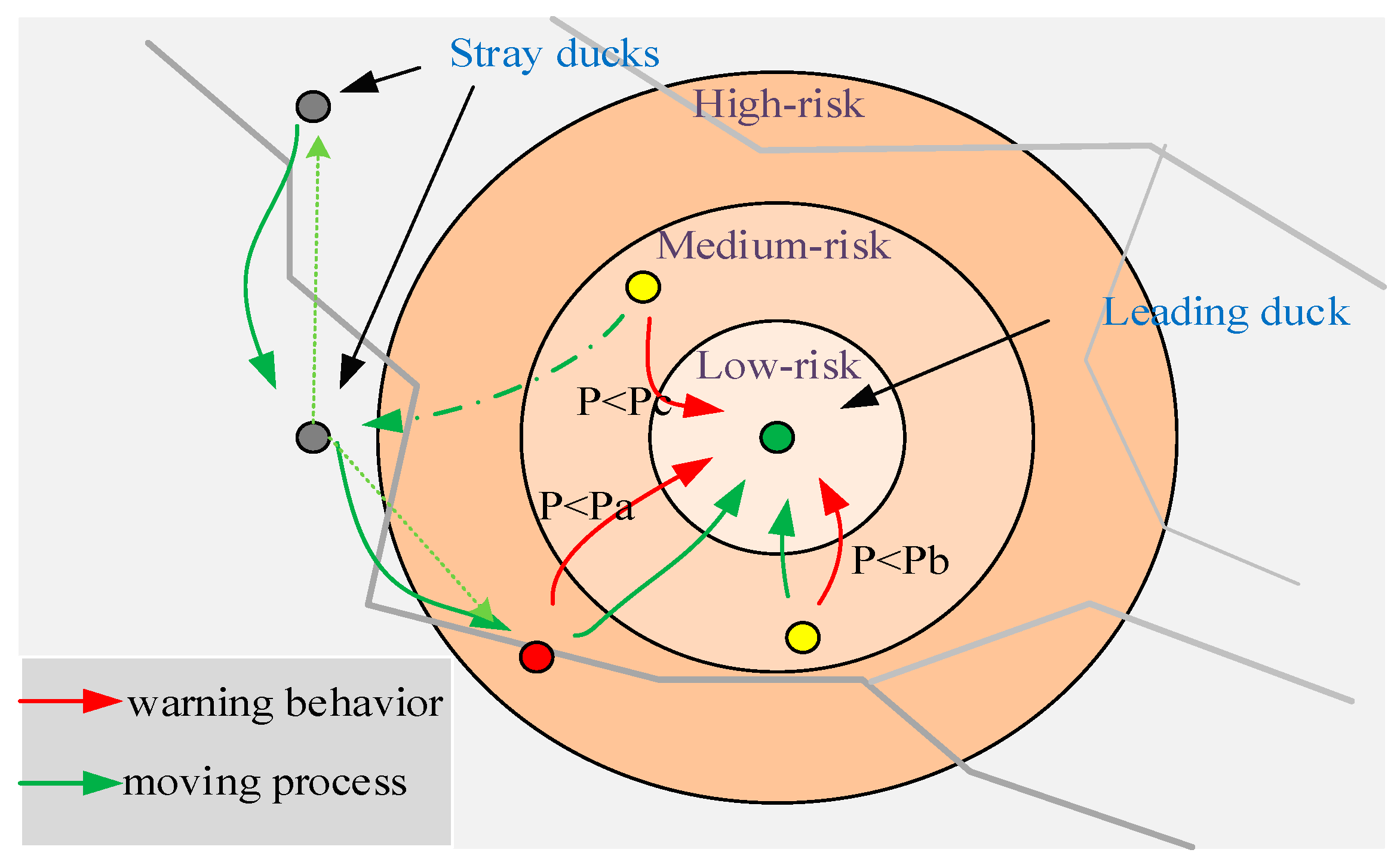
Figure 1. The warning behavior and the moving process of anas platyrhynchos swarm.
Applsci 10 04821 g001
Figure 2. 2D and 3D position vectors and their succeeding possible positions.
Applsci 10 04821 g002
Figure 3. Search history and track of the first particle in the first dimension (part).
Applsci 10 04821 g003aApplsci 10 04821 g003b
Figure 4. Evolution curves of the fitness value for some of the functions in Table 2.
Applsci 10 04821 g004aApplsci 10 04821 g004b
Figure 5. Evolution curves of the fitness value for some of the functions in Table 3.
Applsci 10 04821 g005
Figure 6. Terrain threat map.
Applsci 10 04821 g006
Figure 7. The specific flow of the multi-UAVs cooperative path planning based on APO.
Applsci 10 04821 g007
Figure 8. The result of case 1. (a) 3D UAV cooperative path map; (b) contour map of cooperative path; (c) convergence curve of each UAV; (d) path cost convergence curve.
Applsci 10 04821 g008
Figure 9. The result of case 2. (a) 3D UAV cooperative path map; (b) Contour map of cooperative path; (c) Convergence curve of each UAV; (d) Path cost convergence curve.
Applsci 10 04821 g009
Figure 10. The result of case 3. (a) 3D UAV cooperative path map; (b) contour map of cooperative path; (c) convergence curve of each UAV; (d) path cost convergence curve.
Applsci 10 04821 g010
Figure 11. The result of case 4. (a) 3D UAV cooperative path map; (b) contour map of cooperative path; (c) convergence curve of each UAV; (d) path cost convergence curve.
Applsci 10 04821 g011
Figure 12. The convergence curve of the 3D-integrated path cost of each case. (a) case 1; (b) case 2; (c) case 3; (d) case 4.
Applsci 10 04821 g012
Figure 13. The distribution of the operation results (30 times of testing) of each case. (a) case 1; (b) case 2; (c) case 3; (d) case 4.
Applsci 10 04821 g013
Table 1. Pseudo code of the anas platyrhynchos optimizer (APO).
Setting:low, up, N, D, ObjFun, and T
 Initial population according to Equation (1)
 Calculating fitness function of population by f i t ( P o p i ) = O b j F u n ( P o p i )
 Finding the leading duck P o p b e s t
t = 1
while (t < = T)
  Calculating the Pc according to Equation (2)//warning behavior
  for i from 1 to N do
    if rand < Pc
    Updating position according to Equation (3)
   end if
    Updating parameters A and C according to Equations (8) and (9)//moving process
    Updating position according to Equation (7)
    if f i t ( P o p i ) _ n e w > f i t ( P o p i ) _ o l d //take the minimum as an example
     Selecting another particle P o p r a n d at random
     if f i t ( P o p i > f i t ( P o p r a n d ) )
      Updating position according to Equation (11)
    elseif f i t ( P o p i = f i t ( P o p r a n d ) )
      Keeping unchanged
    elseif f i t ( P o p i < f i t ( P o p r a n d ) )
      Updating position according to Equation (12)
    end if
   end if
  end for
  Finding the leading duck P o p b e s t
t = t + 1
end while
return P o p b e s t
Table 2. High-dimensional benchmark functions used in Test 1.
Test FunctionDRangeOptimum
f 1 ( x ) = i = 1 n x i 2 30[−100,100]0
f 2 ( x ) = i = 1 n | x i | + i = 1 n | x i | 30[−10,10]0
f 3 ( x ) = i = 1 n ( j 1 i x j ) 2 30[−100,100]0
f 4 ( x ) = m a x i { | x i | , 1 i n } 30[−100,100]0
f 5 ( x ) = i = 1 n 1 [ 100 ( x i + 1 x i 2 ) 2 + ( x i 1 ) 2 ] 30[−30,30]0
f 6 ( x ) = i = 1 n ( [ x i + 0.5 ] ) 2 30[−100,100]0
f 7 ( x ) = i = 1 n i x i 4 + r a n d o m [ 0 , 1 ) 30[−1.28,1.28]0
f 8 ( x ) = i = 1 n x i sin ( | x i | ) 30[−500,500]−418.9825∗5
f 9 ( x ) = i = 1 n [ x i 2 10 cos ( 2 π x i ) + 10 ] 30[−5.12,5.12]0
f 10 ( x ) = 20 e x p ( 0.2 1 n i = 1 n x i 2 ) exp ( 1 n i = 1 n cos ( 2 π x i ) ) + 20 + e 30[−32,32]0
f 11 ( x ) = 1 4000 i = 1 n x i 2 i = 1 n cos ( x i i ) + 1 30[−600,600]0
f 12 ( x ) = π n { 10 sin ( π y 1 ) + i = 1 n 1 ( y i 1 ) 2 [ 1 + 10 s i n 2 ( π y i + 1 ) ] + ( y n 1 ) 2 } + i = 1 n u ( x i , 10 , 100 , 4 )
y i = 1 + x i + 1 4
u ( x i , a , k , m ) = { k ( x i a ) m     x i > a 0 a < x i < a k ( x i a ) m     x i < a
30[−50,50]0
f 13 ( x ) = 0.1 { s i n 2 ( 3 π x i ) + i = 1 n ( x i 1 ) 2 [ 1 + s i n 2 ( 3 π x i + 1 ) ] + ( x n 1 ) 2 [ 1 + s i n 2 ( 2 π x n ) ] } + i = 1 n u ( x i , 5 , 100 , 4 ) 30[−50,50]0
D: dimension, range: limits of search space, optimum: global optimal value.
Table 3. Low-dimensional benchmark functions used in Test 1.
f 14 ( x ) = ( 1 500 + j = 1 25 1 j + i = 1 2 ( x i a i j ) 6 ) 1 2[−65,65]1
f 15 ( x ) = i = 1 11 [ a i x 1 ( b i 2 + b i x 2 ) b i 2 + b i x 3 + x 4 ] 2 4[−5,5]0.00030
f 16 ( x ) = 4 x 1 2 2.1 x 1 4 + 1 3 x 1 6 + x 1 x 2 4 x 2 2 + 4 x 2 4 2[−5,5]−1.0316
f 17 ( x ) = ( x 2 5.1 4 π x 1 2 + 5 π x 1 6 ) 2 + 10 ( 1 1 8 π ) cos x 1 + 10 2[−5,5]0.398
f 18 ( x ) = [ 1 + ( x 1 + x 2 + 1 ) 2 ( 19 14 x 1 + 3 x 1 2 ) ] × [ 30 + ( 2 x 1 3 x 2 ) 2 × ( 18 32 x 1 + 12 x 1 2 + 48 x 2 36 x 1 x 2 + 27 x 2 2 ) ] 2[−2,2]3
f 19 ( x ) = i = 1 4 c i e x p ( j = 1 3 a i j ( x j p i j ) 2 ) 3[1,3]−3.86
f 20 ( x ) = i = 1 4 c i e x p ( j = 1 6 a i j ( x j p i j ) 2 ) 6[0,1]−3.32
f 21 ( x ) = i = 1 5 [ ( X a i ) ( X a i ) T + c i ] 1 4[0,10]−10.1532
f 22 ( x ) = i = 1 7 [ ( X a i ) ( X a i ) T + c i ] 1 4[0,10]−10.4028
f 23 ( x ) = i = 1 10 [ ( X a i ) ( X a i ) T + c i ] 1 4[0,10]−10.5363
D: dimension; range: limits of search space; optimum: global optimal value.
Table 4. The parameter settings for the other compared algorithms.
AlgorithmsParameter Settings
Gray wolf optimization (GWO) [8]a = 2 − t*2/T
Whale optimization algorithm (WOA) [9]a1 = 2 − t*2/T, a2 = −1 + t*(−1)/T
Particle swarm optimization (PSO) [2]wmax = 0.9, wmin = 0.2, c1 = c2 = 2
Differential evolution (DE) [68]F = 0.5, CR = 0.9
Table 5. Best, worst, mean, and SD obtained on functions from Table 2.
FResultAPOGWOWOAPSODERank
f1Best7.8190 × 10 145 1.0102 × 10 29 1.9587 × 10 80 9.3358 × 10 6 2.3626 × 10 6 1
Worst6.9690 × 10 108 1.6995 × 10 26 7.1646 × 10 63 0.00292.1183 × 10 4
Mean2.3236 × 10 109 2.1408 × 10 27 2.8808 × 10 64 2.6064 × 10 4 3.3728 × 10 5
Std1.2723 × 10 108 4.1907 × 10 27 1.3261 × 10 63 5.4256 × 10 4 4.4013 × 10 5
f2Best5.5304 × 10 93 1.1204 × 10 17 2.0437 × 10 56 0.00365.1036 × 10 4 1
Worst2.4478 × 10 73 3.6284 × 10 16 3.4372 × 10 46 0.12010.0033
Mean1.3539 × 10 74 9.5431 × 10 17 2.0876 × 10 47 0.03090.0016
Std5.2303 × 10 74 8.7339 × 10 17 7.4074 × 10 47 0.02686.9524 × 10 4
f3Best1.5871 × 10 99 1.1907 × 10 63 4.7969 × 10 12 5.4371 × 10 27 2.2540 × 10 35 1
Worst8.1085 × 10 78 5.6634 × 10 50 0.02935.0743 × 10 22 1.8224 × 10 29
Mean6.0509 × 10 79 2.0580 × 10 51 0.00333.7279 × 10 23 1.6513 × 10 30
Std1.7318 × 10 78 1.0323 × 10 50 0.00681.1100 × 10 22 3.9570 × 10 30
f4Best1.2424 × 10 16 6.5653 × 10 8 5.30460.57315.71232
Worst0.03121.9500 × 10 6 89.62191.522237.5491
Mean0.00295.7114 × 10 7 59.64141.122616.8984
Std0.00784.6159 × 10 7 29.38200.25227.2691
f5Best0.007826.043427.146525.311519.05801
Worst28.780728.748528.8434188.8556181.2647
Mean26.697127.286428.363685.173356.5542
Std7.25740.71670.446640.542540.1468
f6Best1.2702 × 10 6 1.3209 × 10 4 0.73747.9911 × 10 6 3.6153 × 10 6 1
Worst4.3859 × 10 5 1.51193.19814.1143 × 10 4 1.8978 × 10 4
Mean1.3972 × 10 5 0.66021.95569.7234 × 10 5 4.7963 × 10 5
Std9.8769 × 10 6 0.36920.65768.7218 × 10 5 4.8581 × 10 5
f7Best1.9336 × 10 5 4.8037 × 10 4 6.4622 × 10 5 0.08040.03601
Worst0.00770.00340.01940.34690.1085
Mean8.5533 × 10 4 0.00190.00500.17290.0797
Std0.00157.0049 × 10 4 0.00570.05840.0158
f8Best−12569−7250.9N/A−8727.2−7317.71
Worst−12150−3727.9N/A−2629.0−4691.7
Mean−12529−6129.3N/A−4978.3−5946.6
Std106.3406767.8156N/A1569.8667.0457
f9Best05.6843 × 10 14 033.88621.4607 × 10 2 1
Worst016.92675.6843 × 10 14 83.69922.1638 × 10 2
Mean04.05261.8948 × 10 15 58.15071.8134 × 10 2
Std04.50061.0378 × 10 14 14.430616.9916
f10Best8.8818 × 10 16 5.7732 × 10 14 8.8818 × 10 16 0.00165.7932 × 10 4 1
Worst7.9936 × 10 15 1.3589 × 10 13 7.9936 × 10 15 1.51750.0226
Mean2.6645 × 10 15 1.0309 × 10 13 3.8488 × 10 15 0.17570.0024
Std2.2372 × 10 15 1.7645 × 10 14 2.6526 × 10 15 0.43130.0040
f11Best0001.2377 × 10 6 1.5597 × 10 5 1
Worst00.03840.15080.02460.0340
Mean00.00300.00860.00710.0032
Std00.00900.03330.00810.0072
f12Best8.3024 × 10 8 0.00630.02951.3634 × 10 7 5.3389 × 10 6 1
Worst0.00650.09390.72030.10378.3340 × 10 2
Mean2.1901 × 10 4 0.03730.14730.010462.5083
Std0.00120.01860.17220.03161.9621 × 10 2
f13Best1.9591 × 10 6 0.21590.60671.8128 × 10 6 1.0309 × 10 5 1
Worst4.1407 × 10 5 1.14421.95710.01787.4778 × 10 2
Mean1.1372 × 10 5 0.64581.33590.005726.6912
Std1.0199 × 10 5 0.24860.37310.00581.3623 × 10 2
Table 6. Best, worst, wean, and SD obtained on functions from Table 3.
FResultAPOGWOWOAPSODERank
f14Best0.99800.99800.99800.99800.99804
Worst12.670512.670510.763210.76322.9821
Mean4.29734.49372.08223.16361.0641
Std4.00394.00862.14402.85500.3622
f15Best3.1012 × 10 4 3.0749 × 10 4 3.2572 × 10 4 5.0404 × 10 4 3.0749 × 10 4 1
Worst0.00230.02040.00430.00110.0204
Mean5.2403 × 10 4 0.00370.00128.2951 × 10 4 0.0018
Std5.1504 × 10 4 0.00768.6353 × 10 4 1.5813 × 10 4 0.0051
f16Best−1.0316−1.0316−1.0316−1.0316−1.0316=
Worst−1.0316−1.0316−1.0316−1.0316−1.0316
Mean−1.0316−1.0316−1.0316−1.0316−1.0316
Std8.4272 × 10 9 1.7842 × 10 8 2.1111 × 10 9 6.3877 × 10 16 6.7752 × 10 16
f17Best0.39790.39790.39790.39790.3979=
Worst0.39790.39790.39790.39790.3979
Mean0.39790.39790.39790.39790.3979
Std9.2877 × 10 7 2.0274 × 10 4 1.4524 × 10 5 00
f18Best3.00003.00003.00003.00003.0000
Worst30.00003.000030.00333.00003.0000
Mean6.60003.00003.90033.00003.0000
Std9.33514.3052 × 10 5 4.93011.6472 × 10 15 2.0301 × 10 15
f19Best−3.8628−3.8628−3.8628−3.8628−3.8628
Worst−3.8549−3.8549−3.8445−3.8628−3.8628
Mean−3.8605−3.8613−3.8611−3.8628−3.8628
Std0.00360.00270.00382.5829 × 10 15 2.7101 × 10 15
f20Best−3.3220−3.3220−3.3218−3.3220−3.3220
Worst−3.0839−3.0499−3.1627−3.2031−3.2031
Mean−3.2599−3.2672−3.2599−3.2784−3.2507
Std0.08380.08610.06510.05830.0592
f21Best−10.1532−10.1529−10.1526−10.1532−10.15321
Worst−0.8810−2.6302−2.6020−2.6305−2.6305
Mean−9.5341−8.8857−8.2591−7.0685−9.4850
Std2.35222.37092.93353.14092.0722
f22Best−10.4029−10.4025−10.4009−10.4029−10.40291
Worst−10.3988−5.0876−1.8302−2.7519−3.7243
Mean−10.4015−10.2239−7.45423.1828−10.1803
Std0.00110.97013.0686−8.23241.2193
f23Best−10.5364−10.5360−10.5363−10.5364−10.53641
Worst−10.5303−2.4217−1.6447−2.4217−2.8711
Mean−10.5348−10.2638−6.9538−9.5065−10.0575
Std0.00151.48113.74702.38631.8268
Table 7. The results of Wilcoxon signed ranks test based on the solution for each benchmark with 30 independently runs.
FunctionsAPO Versus GWOAPO Versus WOAAPO Versus PSOAPO Versus DE
f11.7344 × 10 6 1.7344 × 10 6 1.7344 × 10 6 1.7344 × 10 6
f21.7344 × 10 6 1.7344 × 10 6 1.7344 × 10 6 1.7344 × 10 6
f31.7344 × 10 6 1.7344 × 10 6 1.7344 × 10 6 1.7344 × 10 6
f40.00391.7344 × 10 6 1.7344 × 10 6 1.7344 × 10 6
f56.6392 × 10 4 0.11568.4661 × 10 6 0.0018
f61.7344 × 10 6 1.7344 × 10 6 5.7517 × 10 6 1.6046 × 10 4
f72.4118 × 10 4 1.6046 × 10 4 1.7344 × 10 6 1.7344 × 10 6
f81.7344 × 10 6 1.7344 × 10 6 1.7344 × 10 6 1.7344 × 10 6
f91.7224 × 10 6 11.7344 × 10 6 1.7344 × 10 6
f101.6521 × 10 6 0.06231.7344 × 10 6 1.7344 × 10 6
f110.50000.12501.7344 × 10 6 1.7344 × 10 6
f121.7344 × 10 6 1.7344 × 10 6 0.01325.2165 × 10 6
f131.7344 × 10 6 1.7344 × 10 6 2.1266 × 10 6 1.7344 × 10 6
f140.54400.05190.20591.7344 × 10 6
f150.08594.1955 × 10 4 0.00280.0859
f161.0570 × 10 6 0.07861.7344 × 10 6 1.7344 × 10 6
f178.9443 × 10 6 6.9838 × 10 6 1.7344 × 10 6 1.7344 × 10 6
f181.9209 × 10 6 1.4936 × 10 6 1.7344 × 10 6 1.7344 × 10 6
f190.89360.55771.7344 × 10 6 1.7344 × 10 6
f200.50380.21340.02850.8130
f210.00131.8910 × 10 4 0.04490.0018
f220.03001.7344 × 10 6 0.64353.1123 × 10 5
f230.03505.2165 × 10 6 0,05710.0350
Table 8. Model parameters of peaks.
NumberAltitude (m)Center Location (x,y)/(km)Slope
1130(56,82)(10,10)
2150(75,20)(10,10)
3300(50,45)(12,12)
4100(22,20)(8,8)
5150(20,70)(8,8)
6150(77,73)(10,10)
Table 9. Coordinates of the starting and target points of all UAVs (case 1).
NumberStart PointTarget Point
1(1,1,0)(100,30,70)
2(1,30,0)(100,40,70)
3(1,60,0)(100,50,70)
Table 10. Range and flight time of each aircraft (case 1).
NumberRange (km)Flight Time (s)
1110.9405[1849.0089, 2773.5134]
2102.1812[1703.0205, 2554.5307]
3102.259[1704.3164, 2556.4746]
Table 11. Coordinates of the starting and target points of all UAVs (case 2).
NumberStart PointTarget Point
1(1,1,0)(90,40,100)
2(1,30,0)(95,40,100)
3(1,55,0)(95,85,100)
4(1,90,0)(80,85,100)
Table 12. Range and flight time of each aircraft (case 2).
NumberRange (km)Flight Time (s)
1117.7185[1961.975, 2942.9626]
299.8391[1663.9855, 2495.9783]
3106.0902[1768.1699, 2652.2548]
497.3108[1621.8469, 2432.7704]
Table 13. Coordinates of the starting and target points of all UAVs (case 3).
NumberStart PointTarget Point
1(1,1,0)(99,10,70)
2(1,20,0)(99,18,70)
3(1,40,0)(99,30,70)
4(1,60,0)(99,40,70)
5(1,75,0)(99,70,70)
6(1,90,0)(99,90,70)
Table 14. Range and flight time of each aircraft (case 3).
NumberRange (km)Flight Time(s)
199.2486[1654.1433, 2481.215]
2104.8832[1748.0538, 2622.0807]
3115.4467[1924.111, 2886.1664]
4110.7951[1846.5853, 2769.8779]
5104.5509[1742.5156, 2613.7734]
6100.002[1666.7006, 2500.0509]
Table 15. Coordinates of the starting and target points of all UAVs (case 4).
NumberStart PointTarget Point
1(1,1,0)(99,10,70)
2(1,15,0)(99,10,70)
3(1,30,0)(99,32,70)
4(1,40,0)(99,32,70)
5(1,55,0)(99,68,70)
6(1,70,0)(99,68,70)
7(1,80,0)(99,85,70)
8(1,95,0)(99,85,70)
Table 16. Range and flight time of each aircraft (case 4).
NumberRange (km)Flight Time (s)
199.7531[1662.5517, 2493.8276]
2100.9139[1681.8984, 2522.8476]
3115.3703[1922.8382, 2884.2573]
4101.3747[1689.5775, 2534.3663]
5101.0788[1684.6466, 2526.97]
6102.4978[1708.2963, 2562.4445]
7103.6654[1727.7567, 2591.635]
8100.3576[1672.6264, 2508.9396]
Table 17. The parameter settings for the other compared algorithms.
AlgorithmsParameter Settings
APOa = 2 − t*2/T
GWO, HGWO, IGWOa = 2 − t*2/T
PSOwmax = 0.9, wmin = 0.2, c1 = c2 = 2
DEF = 0.5, CR = 0.9
Table 18. The average time of each algorithm in each case (unit: s).
CaseAPOGWOHGWOIGWOPSODE
15.12685.69727.117556.677414.017127.2034
27.57168.17829.940764.227619.213138.6358
312.738612.484215.82965.768733.388661.1923
418.722918.858121.822481.917245.5781.6728