Human Skeleton Data Augmentation for Person Identification over Deep Neural Network

Abstract

With the advancement in pose estimation techniques, skeleton-based person identification has recently received considerable attention in many applications. In this study, a skeleton-based person identification method using a deep neural network (DNN) is investigated. In this method, anthropometric features extracted from the human skeleton sequence are used as the input to the DNN. However, training the DNN with insufficient training datasets makes the network unstable and may lead to overfitting during the training phase, causing significant performance degradation in the testing phase. To cope with a shortage in the dataset, we investigate novel data augmentation for skeleton-based person identification by utilizing the bilateral symmetry of the human body. To achieve this, augmented vectors are generated by sharing the anthropometric features extracted from one side of the human body with the other and vice versa. Thereby, the total number of anthropometric feature vectors is increased by 256 times, which enables the DNN to be trained while avoiding overfitting. The simulation results demonstrate that the average accuracy of person identification is remarkably improved up to 100% based on the augmentation on public datasets.

1. Introduction

Biometric-based person identification systems have attracted considerable attention owing to their advantages in a wide range of applications, such as access control, home security monitoring, surveillance, and personalized customer services [1,2,3], where accuracy in the identification of individuals is paramount. To achieve this goal, various biometric technologies have been developed, such as ear, face, fingerprint, gait, iris, palmprint, and voice [4,5,6,7,8,9,10]. According to the type of biometric information used, these technologies can be categorized into active and passive systems. In the active system, the user is required to make physical contact with a certain interface or device for the extraction of biometric information. Fingerprint-, iris-, and palmprint-based person identification systems are prime examples of the active system. By contrast, in the passive system, the biometric information of the user is extracted at a distance by utilizing sensor data without the need for physical contact. Ear-, face-, gait-, and voice-based person identification systems are prime examples of the passive system.

Although no physical contact is required, it is necessary to have the cooperation of the user to enable recognition of their ear, face, and voice. To clarify, suppose a user has long hair that covers their ears and wears a facemask and hat that conceal parts of the face, it is difficult to clearly recognize the ears and face owing to the occlusion. To improve the accuracy, cooperation with the person identification process would be necessary. However, the user may feel uncomfortable to reveal their ears and remove the facemask and hat to reveal their face. For voice recognition, the user needs to say a few sentences into a sensor even if they are reluctant to say anything.

By contrast, gait recognition has the advantage of being performed without the user’s cooperation, wherein the user only has to walk in the usual way. Because the user’s gait data can be obtained from a video filmed from a far or close distance, the person identification process is performed in such a way that the user is unaware and does not feel uncomfortable. Owing to such an advantage, gait recognition has gained significant interest of researchers in the computer-vision community. Early studies, including [11,12,13,14,15], adopted the approach of extracting the user’s gait information from the silhouette sequence. In addition, in most of these studies, only the silhouette sequence extracted from a video in which a walking person was photographed from a side view was used. It may be relatively easy to identify a person using the gait information extracted from the side view of a walking person. However, from the frontal viewpoint, the ability to identify the person accurately is limited.

The software development kit (SDK) of the Microsoft Kinect sensor was released in May 2011 [16]. Using the SDK, the user can acquire three-dimensional (3D) position data for 20 joints of the human body from the Kinect sensor [17,18,19]. In comparison with the human silhouette, the use of joint position enables view-invariant person identification. Using this advantage, several studies on person identification methods have been conducted using the Kinect sensor. Munsell et al. [20] acquired human skeleton data from walking and running people to achieve person identification. The authors calculated the difference in motion between unknown and authenticated people using their skeleton data. Wu et al. [21] compared the performance of silhouette- and Kinect skeleton-based person identification methods, which revealed that using the skeleton data was a more reliable method for person identification.

The use of skeleton data created a new modality for biometric features, called the anthropometric feature, for person identification. In [22,23,24,25,26,27,28], the authors proposed the use of anthropometric features for the person identification task. In most of these studies, several machine-learning algorithms, such as k-nearest neighbor (k-NN), support vector machine (SVM), and multi-layer perceptron (MLP), were used to identify individuals using the anthropometric features. In addition, it was observed that k-NN outperformed the other algorithms in terms of accuracy.

Recently, deep learning has been successfully implemented in various fields, such as computer vision, and natural language processing [29,30,31,32]. In addition, many studies showed that deep learning outperforms other traditional machine learning methods, such as k-NN and SVM [33,34,35,36,37]. Therefore, as long as the diversity of dataset is guaranteed to represent the person identification, it could achieve higher identification accuracy than using traditional machine learning methods. To this end, first of all, we explored the dataset that was used in previous studies [22,23,24,25]. From this investigation, we observed the overfitting that caused significant performance degradation. In addition, we revealed that the size of the dataset was too small for deep learning. To cope with the shortage in the dataset, it is necessary to develop a method capable of increasing the data. However, to the best of our knowledge, research on data augmentation for person identification has not yet been conducted.

In this study, we propose a novel data augmentation method based on the bilateral symmetry of the human body to resolve the data shortage issue that causes overfitting during the training phase. This method is applied to each anthropometric feature vector extracted from the Kinect skeleton sequence. Using this method, the total number of anthropometric feature vectors is increased 256 times. Furthermore, we propose a simple but effective deep neural network (DNN) for person identification. To verify the effectiveness of the algorithm, we conduct benchmarking on the existing person identification dataset.

The remainder of this paper is organized as follows. In Section 2, a review of the related work is presented. In Section 3, the motivation for our study is discussed. In Section 4, the 3D human skeleton model is presented and the anthropometric features are formulated. The proposed data augmentation method and DNN architecture are described in Section 5. In Section 6 and Section 7, the simulation results and discussion are presented, respectively. Conclusions are made in Section 8.

2. Related Work

The idea of using anthropometric features in person identification was first proposed by Araujo et al. [22]. The authors calculated the length of 11 human body parts captured by the Kinect sensor. The parts used were as follows: (1) left and right upper arms, (2) left and right forearms, (3) left and right shanks, (4) left and right thighs, (5) thoracic spine, (6) cervical spine, and (7) height. Using the average length of each body part, the authors tested four learning algorithms, including MLP and k-NN, on their own data consisting of eight subjects. According to their results, k-NN outperformed the other algorithms, achieving about $99.6\%$ accuracy.

Andersson et al. [23] investigated the usefulness of the anthropometric features on large-scale datasets. After capturing skeleton data from 164 individuals using the Kinect sensor, they tested the two learning algorithms, MLP and k-NN, on their own data. The results showed that as the number of subjects for identification increased, the accuracy of both the algorithms decreased. From the evaluation with different numbers of subjects, it was shown that k-NN always outperformed MLP. Andersson et al. [24] extended their previous work by exploring the effect of different numbers of subjects on the person identification accuracy. In addition, to improve the accuracy, they proposed to use the anthropometric features for all limbs rather than for only a limited number of limbs. As a result, 20 anthropometric features, including average lengths of the left and right shoulders, hands, hips, and feet, were used for person identification. Using these features, the authors tested three learning algorithms: SVM, k-NN, and MLP. As the number of subjects for identification increased by 15, in the range from 5 to 140, the accuracy of all the algorithms decreased. The k-NN algorithm outperformed the other algorithms except when the number of subjects was less than 35. By utilizing the extended anthropometric features, the accuracy of k-NN increased from approximately $80\%$ [23] to approximately $85.4\%$ [24].

The same authors analyzed their previous results in a subsequent study [25]. Focusing on k-NN, they explored the importance of each anthropometric feature to identify individuals. By removing each anthropometric feature without repetition of the measurement, the authors measured the average accuracy of k-NN using the remaining features. In addition, the importance of the corresponding feature was assessed by calculating the decrease in the average accuracy. From the results, the importance of the anthropometric features in person identification was seen to differ for different features. According to their results, the average length of the right foot was the most important anthropometric feature utilized to identify individuals. Motivated by these results, Yang et al. [26] proposed to apply the majority voting method to the person identification algorithm. In their studies, a person was identified by the voting results of 100 k-NN classifiers. For the training of each k-NN classifier, 10 randomly selected anthropometric features from a total of 20 were used. The authors tested their proposed method on the public person identification dataset proposed by Andersson et al. [25]. The average accuracy could be improved by $2.2\%$ from $83.9\%$ to $86.1\%$ using their voting-based method.

Sun et al. [27] created a connection between 2D silhouette- and 3D skeleton-based person identification methods. Using the Kinect sensor, they built a person identification dataset composed of 2D silhouette and 3D skeleton sequences captured from 52 subjects. In their study, they extracted eight anthropometric features from the 3D skeleton sequences and then calculated a score defined by the weighted sum of the values of features. To determine the weight of each feature, they measured the correct classification rate when the corresponding feature was used for person identification. After the measurement was completed for all features, the authors set the weight of each feature as the corresponding correct classification rate. They trained k-NN using the obtained scores, and tested it on their own dataset.

3. Motivation

As reviewed in Section 2, the three machine-learning algorithms, k-NN, SVM, and MLP, have been widely used for person identification. In general, k-NN demonstrates better performance than the other methods [22,23,24,25]. For verification of the performance, we implemented the MLP as in previous studies [22,23,24,25], which included a single hidden layer. The number of hidden units was set to 10, 20, and 40. We attempted to train the MLP using the simulation parameters used previously [22,23,24,25], but failed to achieve the desired accuracy. From the investigation, we found that the numbers of hidden layers and hidden units of the MLP were too small to learn person identification tasks.

To overcome this issue, we used a DNN that consists of two dense layers with 512 full connections in each layer. With the DNN, the training set can achieve an accuracy of up to almost 100% over the same datasets used previously [22,23,24,25]. Figure 1 shows the training loss and training set accuracy of the DNN. As shown in the figure, after approximately 360 epochs, the training loss converges and the training set accuracy reaches approximately 100%. Nevertheless, the maximum test accuracy of the DNN is 57.5%. From this simulation, we found that overfitting occurs during the training phase, which in turn leads to significant performance degradation in the testing phase.

To overcome the overfitting issue, we applied several techniques such as batch normalization [38], dropout [39], and L2 regularization [40] according to the number of hidden layers and the number of hidden units in each layer. However, we failed to avoid overfitting due to the shortage in the dataset. The dataset contains 160 subjects in total with 5 sequences for each. Therefore, this dataset contains a total number of 800 sequences $(=160\mathrm{subjects}\times 5\mathrm{sequences}\mathrm{per}\mathrm{subject})$. Assuming that 5-fold cross-validation is used, 640 sequences $(=160\mathrm{subjects}\times 4\mathrm{sequences}\mathrm{per}\mathrm{subject})$ can be used for the training, which is insufficient to train the DNN without overfitting.

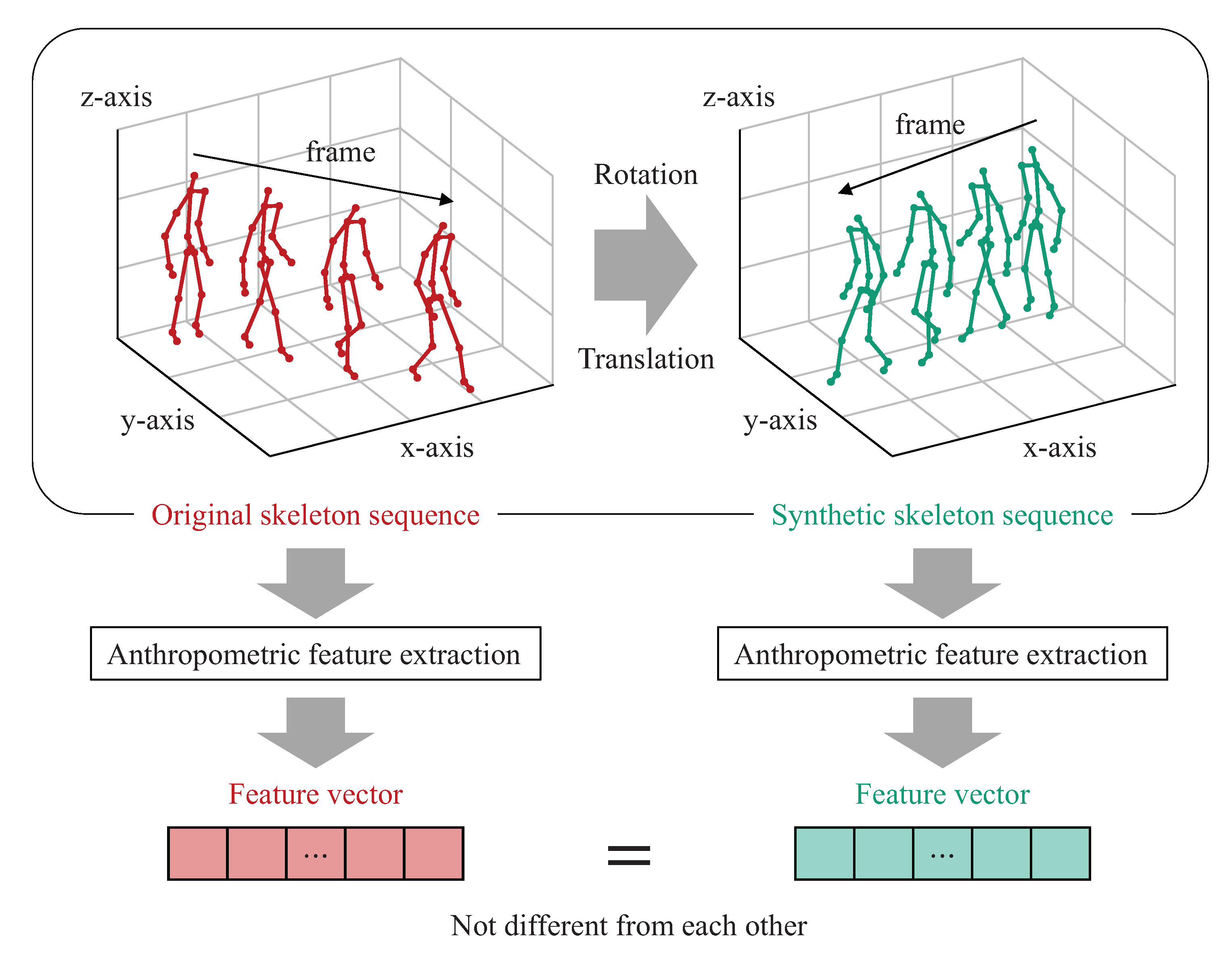
Therefore, to overcome the lack of data, we propose a novel data augmentation method to achieve both training set enrichment and overfitting prevention effectively. For this augmentation, we focus on increasing the number of anthropometric feature vectors rather than the number of 3D skeleton sequences based on the fact that the human body has bilateral symmetry. The main motivation for the approach is as follows: in general, the synthetic skeleton sequence can be generated by rotation and translation in 3D coordinates without loss of information [41,42]. However, even if the number of skeleton sequences increases by generating such personal synthetic skeleton sequences, the anthropometric features extracted from the original and synthetic skeleton sequences are similar, as shown in Figure 2, so that there is a limitation to improve the performance by increasing the synthetic skeleton sequence only. Therefore, it is essential to augment anthropometric feature vectors for training the DNN more accurately while preventing the DNN from overfitting.

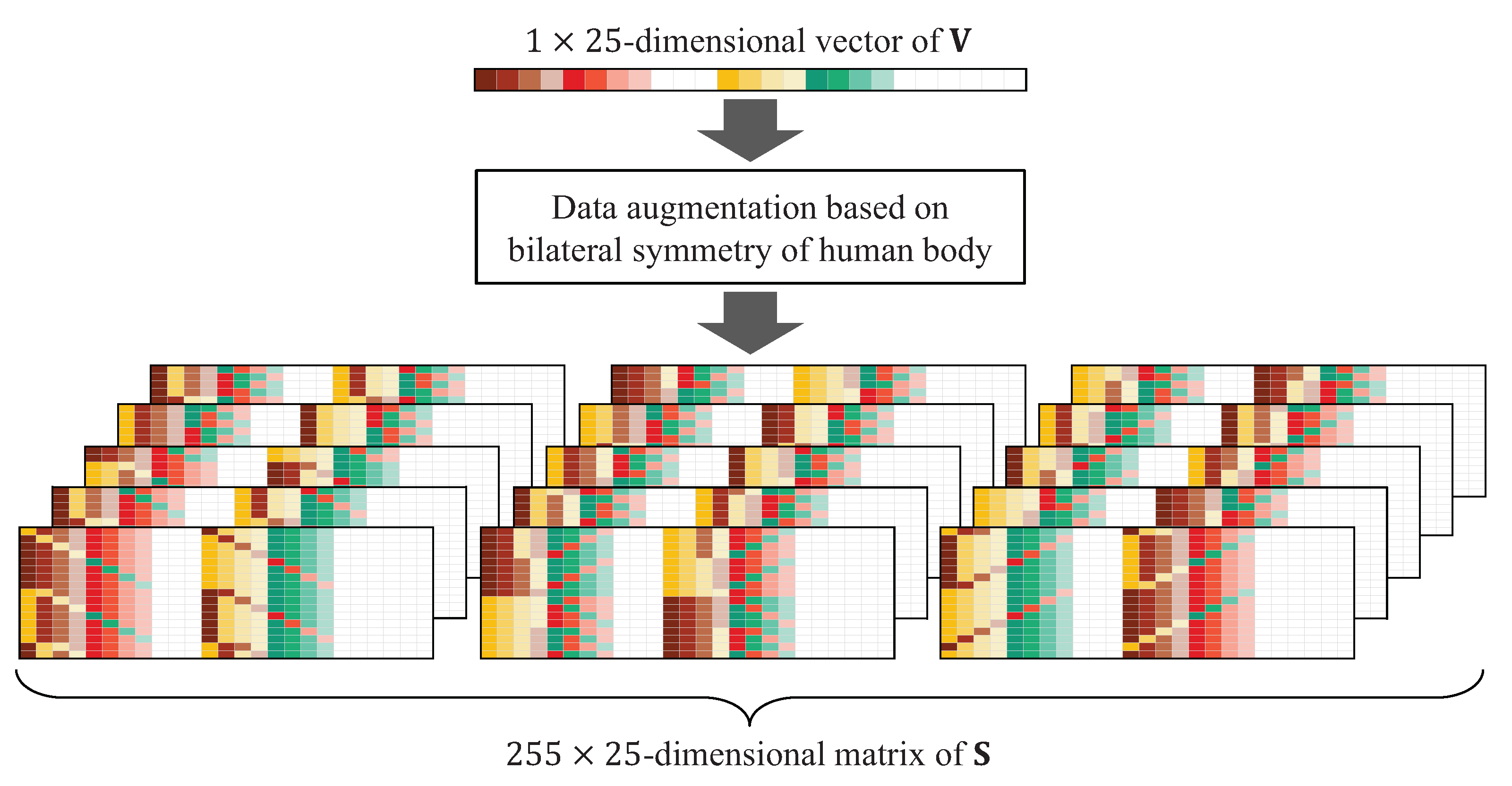
Hence, we note that some of the anthropometric features, such as the average lengths of the left and right arms, forearms, thighs, and shanks, are reflected by the characteristics of bilateral symmetry of the human body. Inspired by this, we utilize this bilateral symmetry for data augmentation, which is highly effective to improve the performance on small-scale datasets. Figure 3 shows a schematic overview of our proposed method for skeleton-based person identification. In the proposed method, for each anthropometric feature vector, we augment new vectors by exchanging the anthropometric features extracted from the left (or right) side of the human body with the corresponding right (or left) features. According to our data augmentation method, for the Kinect skeleton, the size of the anthropometric feature vector set can be increased 256 times. In addition, using these augmented datasets, the DNN can be effectively trained without overfitting. In the next section, the 3D human skeleton model and anthropometric features are described in detail.

4. 3D Human Skeleton Model and Anthropometric Features

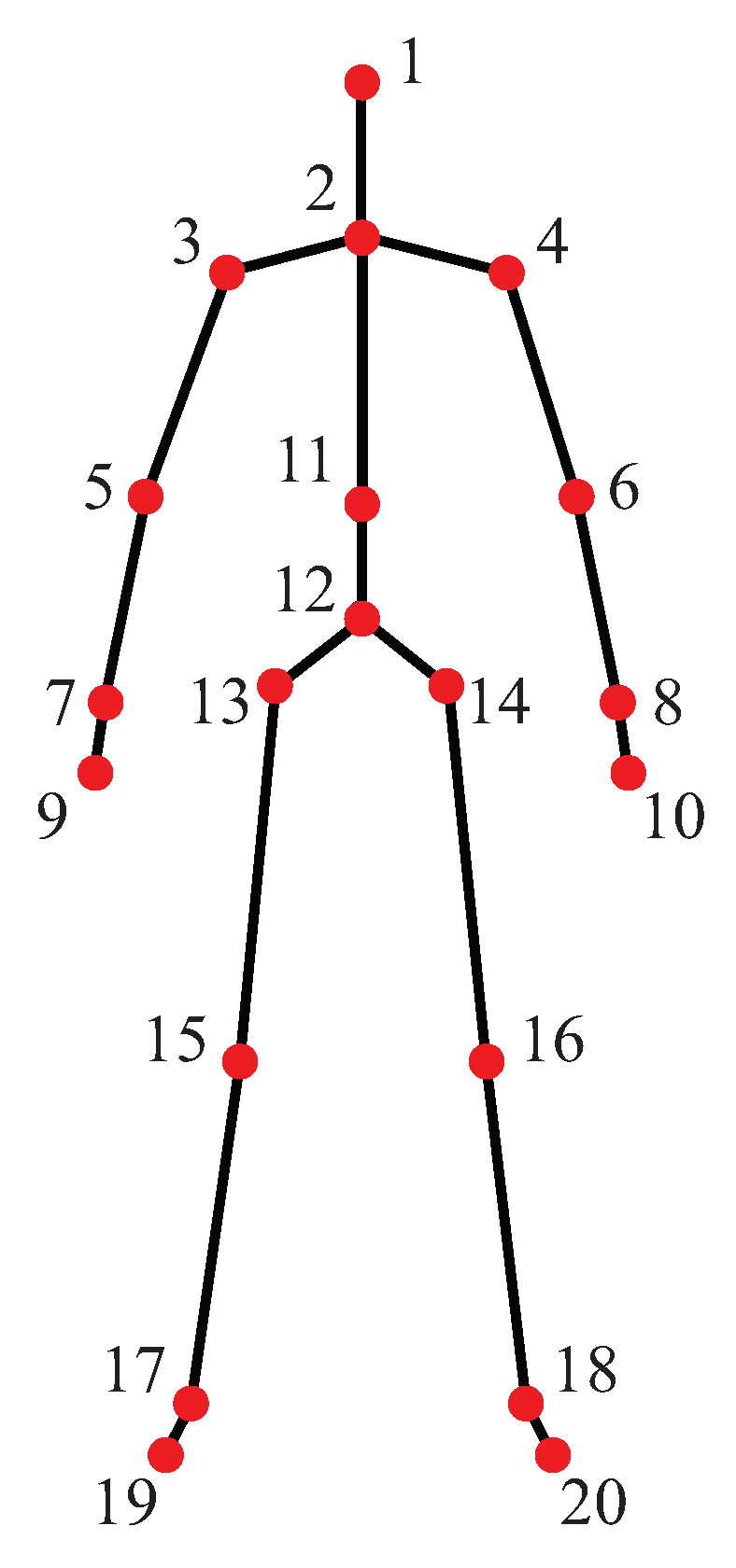
Assume that a 3D human skeleton model consists of N joints with their set of indices $J=\{1,\cdots ,N\}$ and M limbs, which are represented by line segments between two joints. Let $L=\left\{\right(i,j\left)\right|i\ne j,i\in J,j\in J\}$ be the set of joint pairs for constructing the limbs [43]. The values of N and M depend on the product specification of the motion capture sensors. For the Kinect sensor, N and M are 20 and 19, respectively, as shown in Figure 4. The details of the joint and limb information of the Kinect skeleton are provided in

Table 1. Joint information of 3D human skeleton from Kinect sensor.

Joint #	Joint Name	Joint #	Joint Name
1	head	11	spine
2	center of shoulder	12	center of hip
3	right shoulder	13	right hip
4	left shoulder	14	left hip
5	right elbow	15	right knee
6	left elbow	16	left knee
7	right wrist	17	right ankle
8	left wrist	18	left ankle
9	right hand	19	right foot
10	left hand	20	left foot

and

Table 2. Limb information of 3D human skeleton from Kinect sensor.

Limb #	Pair of Joints			$(\mathit{i},\mathit{j})\in \mathit{L}$
1	center of shoulder	–	right shoulder	$(2,3)$
2	right shoulder	–	right elbow	$(3,5)$
3	right elbow	–	right wrist	$(5,7)$
4	right wrist	–	right hand	$(7,9)$
5	center of hip	–	right hip	$(12,13)$
6	right hip	–	right knee	$(13,15)$
7	right knee	–	right ankle	$(15,17)$
8	right ankle	–	right foot	$(17,19)$
9	head	–	center of shoulder	$(1,2)$
10	center of shoulder	–	spine	$(2,11)$
11	spine	–	center of hip	$(11,12)$
12	center of shoulder	–	left shoulder	$(2,4)$
13	left shoulder	–	left elbow	$(4,6)$
14	left elbow	–	left wrist	$(6,8)$
15	left wrist	–	left hand	$(8,10)$
16	center of hip	–	left hip	$(12,14)$
17	left hip	–	left knee	$(14,16)$
18	left knee	–	left ankle	$(16,18)$
19	left ankle	–	left foot	$(18,20)$

, respectively.

Let ${\mathbf{P}}_j=\left[x_j,y_j,z_j\right]$ be the position of the $j\mathrm{th}$ joint in the world coordinate system, where $x_j$, $y_j$, and $z_j$ are the coordinates of the $j\mathrm{th}$ joint on the X-, Y-, and Z-axes, respectively. The Euclidean distance between the $i\mathrm{th}$ and $j\mathrm{th}$ joints $d({\mathbf{P}}_i,{\mathbf{P}}_j)$ is used as a distance feature.

The anthropometric features can be categorized into seven types: (1) length of each limb, (2) height, (3) length of upper body, (4) length of lower body, (5) ratio of upper body length to lower body length, (6) chest size, and (7) hip size. After these values are calculated for each frame, their average values over all frames are used as the anthropometric features for person identification. For the frame index n and the frame length F, the anthropometric feature is defined as follows.

(1) $f_1$: Average length of each limb. In most case, the length of each limb will differ from person to person. For this reason, in many studies, this anthropometric feature has been used for person identification [22,23,24,25,26,27,28]. The length of each limb is calculated for each frame and the average length of each limb over all frames is given by

$$\begin{array}{c}\hfill f_1=\frac{{\sum }_{n=1}^{F}d({\mathbf{P}}_i\left[n\right],{\mathbf{P}}_j\left[n\right])}{F},(i,j)\in L,\end{array}$$

(1)

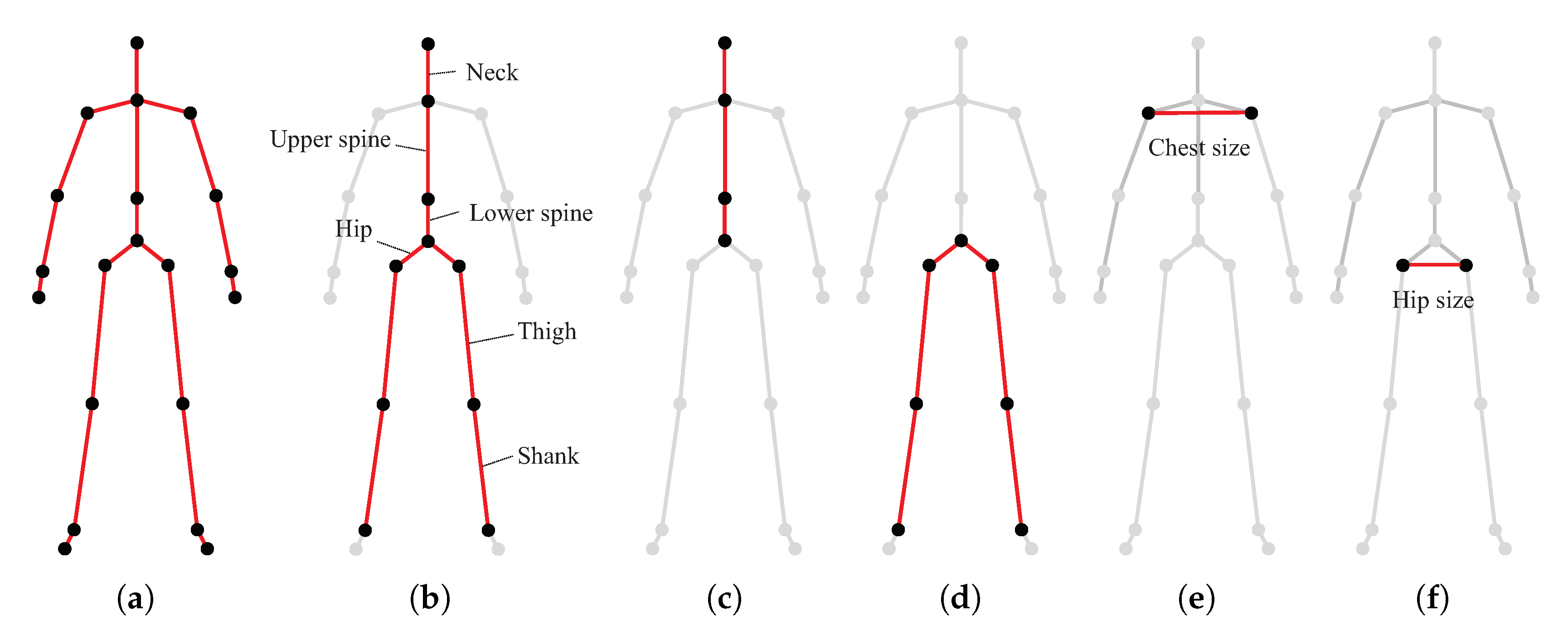
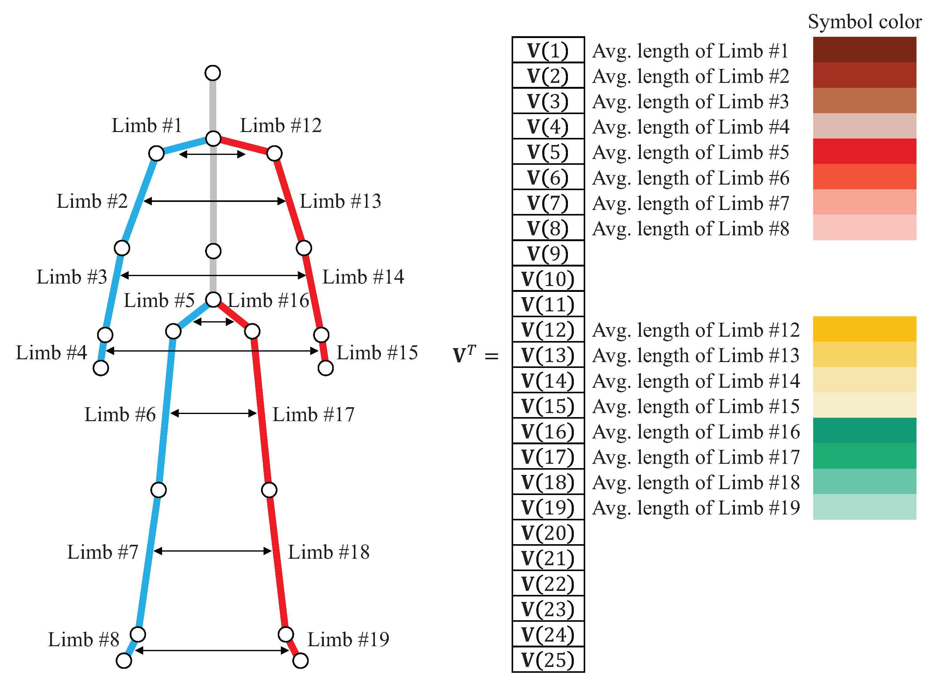
where ${\mathbf{P}}_i\left[n\right]$ and ${\mathbf{P}}_j\left[n\right]$ are the position of the $i\mathrm{th}$ and the $j\mathrm{th}$ joints at the $n\mathrm{th}$ frame, respectively. Since the 19 limbs shown in Figure 5a are used, the number of feature dimensions of $f_1$ becomes 19.

(2) $f_2$: Average height. Human height is also one of the most important anthropometric features used for person identification and is measured as the vertical distance from the foot to the head [22,23,24,25,26,28]. In general, the person is asked to stand up straight while their height is measured. However, for a walking person, it is difficult to measure the true height due to the posture difference. To alleviate this issue, as shown in Figure 5b, the person’s height is calculated as the sum of the neck length, upper and lower spine lengths, and the average lengths of the right and left hips, thighs, and shanks. To clarify, let $H\left[n\right]$ be the subject’s height at the $n\mathrm{th}$ frame. Then, $H\left[n\right]$ is defined by (2) as follows:

$$\begin{array}{cc}H\left[n\right]\hfill & =\underset{=\mathrm{neck}\mathrm{length}}{\underbrace{d({\mathbf{P}}_1\left[n\right],{\mathbf{P}}_2\left[n\right])}}+\underset{=\mathrm{upper}\mathrm{spine}\mathrm{length}}{\underbrace{d({\mathbf{P}}_2\left[n\right],{\mathbf{P}}_{11}\left[n\right])}}+\underset{=\mathrm{lower}\mathrm{spine}\mathrm{length}}{\underbrace{d({\mathbf{P}}_{11}\left[n\right],{\mathbf{P}}_{12}\left[n\right])}}\hfill \\ \hfill & +\underset{=\mathrm{average}\mathrm{length}\mathrm{of}\mathrm{the}\mathrm{right}\mathrm{and}\mathrm{left}\mathrm{hips}}{\underbrace{\{d({\mathbf{P}}_{12}\left[n\right],{\mathbf{P}}_{13}\left[n\right])+d({\mathbf{P}}_{12}\left[n\right],{\mathbf{P}}_{14}\left[n\right])\}/2}}+\underset{=\mathrm{average}\mathrm{length}\mathrm{of}\mathrm{the}\mathrm{right}\mathrm{and}\mathrm{left}\mathrm{thighs}}{\underbrace{\{d({\mathbf{P}}_{13}\left[n\right],{\mathbf{P}}_{15}\left[n\right])+d({\mathbf{P}}_{14}\left[n\right],{\mathbf{P}}_{16}\left[n\right])\}/2}}\hfill \\ \hfill & +\underset{=\mathrm{average}\mathrm{length}\mathrm{of}\mathrm{the}\mathrm{right}\mathrm{and}\mathrm{left}\mathrm{shanks}}{\underbrace{\{d({\mathbf{P}}_{15}\left[n\right],{\mathbf{P}}_{17}\left[n\right])+d({\mathbf{P}}_{16}\left[n\right],{\mathbf{P}}_{18}\left[n\right])\}/2}}.\hfill \end{array}$$

(2)

Using $H\left[n\right]$ in (2), the average height over all frames is obtained by

$$\begin{array}{cc}\hfill f_2& =\frac{{\sum }_{n=1}^{F}H\left[n\right]}{F}.\hfill \end{array}$$

(3)

(3) $f_3$: Average length of upper body. This feature was introduced by Nambiar et al. [44,45]. As shown in Figure 5c, the upper body length is defined as the sum of the neck length and upper and lower spine lengths. Let $U\left[n\right]$ be the upper body length at the $n\mathrm{th}$ frame. Then, $U\left[n\right]$ is defined by

$$\begin{array}{cc}\hfill U\left[n\right]& =\underset{=\mathrm{neck}\mathrm{length}}{\underbrace{d({\mathbf{P}}_1\left[n\right],{\mathbf{P}}_2\left[n\right])}}+\underset{=\mathrm{upper}\mathrm{spine}\mathrm{length}}{\underbrace{d({\mathbf{P}}_2\left[n\right],{\mathbf{P}}_{11}\left[n\right])}}+\underset{=\mathrm{lower}\mathrm{spine}\mathrm{length}}{\underbrace{d({\mathbf{P}}_{11}\left[n\right],{\mathbf{P}}_{12}\left[n\right])}}.\hfill \end{array}$$

(4)

Using $U\left[n\right]$ in (4), the average length of the upper body over F frames becomes

$$\begin{array}{c}\hfill f_3=\frac{{\sum }_{n=1}^{F}U\left[n\right]}{F}\end{array}$$

(5)

(4) $f_4$: Average length of lower body. This feature was introduced by Nambiar et al. [44,45]. As shown in Figure 5d, the lower body length is defined as the sum of the average of the lengths of the right and left hips, thighs, and shanks. The lower body length at the $n\mathrm{th}$ frame $W\left[n\right]$ is then

$$\begin{array}{cc}W\left[n\right]\hfill & =\underset{=\mathrm{average}\mathrm{length}\mathrm{of}\mathrm{the}\mathrm{right}\mathrm{and}\mathrm{left}\mathrm{hips}}{\underbrace{\{d({\mathbf{P}}_{12}\left[n\right],{\mathbf{P}}_{13}\left[n\right])+d({\mathbf{P}}_{12}\left[n\right],{\mathbf{P}}_{14}\left[n\right])\}/2}}+\underset{=\mathrm{average}\mathrm{length}\mathrm{of}\mathrm{the}\mathrm{right}\mathrm{and}\mathrm{left}\mathrm{thighs}}{\underbrace{\{d({\mathbf{P}}_{13}\left[n\right],{\mathbf{P}}_{15}\left[n\right])+d({\mathbf{P}}_{14}\left[n\right],{\mathbf{P}}_{16}\left[n\right])\}/2}}\hfill \\ \hfill & +\underset{=\mathrm{average}\mathrm{length}\mathrm{of}\mathrm{the}\mathrm{right}\mathrm{and}\mathrm{left}\mathrm{shanks}}{\underbrace{\{d({\mathbf{P}}_{15}\left[n\right],{\mathbf{P}}_{17}\left[n\right])+d({\mathbf{P}}_{16}\left[n\right],{\mathbf{P}}_{18}\left[n\right])\}/2}}.\hfill \end{array}$$

(6)

Using $W\left[n\right]$ in (6), the average length of the lower body is

$$\begin{array}{c}\hfill f_4=\frac{{\sum }_{n=1}^{F}W\left[n\right]}{F}.\end{array}$$

(7)

(5) $f_5$: Average ratio of upper body length to lower body length. This feature was introduced by Nambiar et al. [44,45] and is written as

$$\begin{array}{c}\hfill f_5=\frac{{\sum }_{n=1}^F\{U\left[n\right]/W\left[n\right]\}}{F}.\end{array}$$

(8)

(6) $f_6$: Average chest size. As shown in Figure 5f, the chest size is defined as the distance between the third and fourth joints (i.e., right shoulder and left shoulder) [27]. The average chest size is

$$\begin{array}{c}\hfill f_6=\frac{{\sum }_{n=1}^{F}d({\mathbf{P}}_3\left[n\right],{\mathbf{P}}_4\left[n\right])}{F}.\end{array}$$

(9)

(7) $f_7$: Average hip size. As shown in Figure 5e, the hip size is defined as the distance between the $13\mathrm{th}$ and $14\mathrm{th}$ joints (i.e., right and left hips). The average hip size is

$$\begin{array}{c}\hfill f_7=\frac{{\sum }_{n=1}^{F}d({\mathbf{P}}_{13}\left[n\right],{\mathbf{P}}_{14}\left[n\right])}{F}.\end{array}$$

(10)

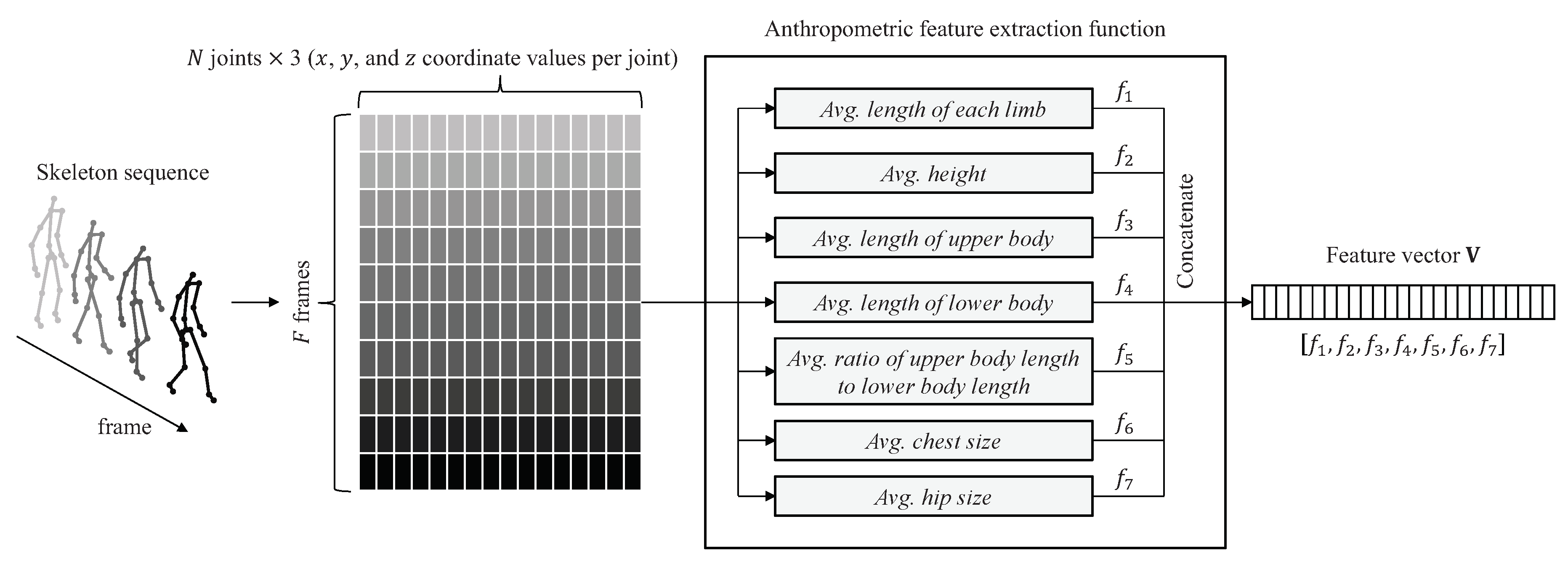
After the anthropometric feature extraction is completed, the extracted features are concatenated into a feature vector as

$$\begin{array}{c}\hfill \mathbf{V}=\left[f_1,f_2,f_3,f_4,f_5,f_6,f_7\right].\end{array}$$

(11)

The dimension of $\mathbf{V}$ is $1\times 25$. Figure 6 shows the procedure to generate $\mathbf{V}$ from the skeleton sequence, which is then inputted to the DNN for identifying individuals.

5. Data Augmentation for Person Identification

5.1. Human Bilateral Symmetry-Based Data Augmentation

Here, we propose a novel data augmentation method by exploiting the bilateral symmetry of the human skeleton structure. In general, the length of the limbs on the left and right sides can be regarded as equal. As shown in Figure 7, eight pairs of limbs in the skeleton are symmetric. Using the limb definition in Table 2, the pairs are denoted as follows: (Limb #1, Limb #12), (Limb #2, Limb #13), (Limb #3, Limb #14), (Limb #4, Limb #15), (Limb #5, Limb #16), (Limb #6, Limb #17), (Limb #7, Limb #18), and (Limb #8, Limb #19). Using Equation (1), the average lengths for these limbs are calculated. In addition, from the feature concatenation process in Figure 6, the calculated values are located from the $1\mathrm{st}$ element to the $8\mathrm{th}$ element, and from the $12\mathrm{th}$ element to the $19\mathrm{th}$ element. Figure 7 depicts the proposed data augmentation method, where $\mathbf{V}\left(t\right)$ is the $t\mathrm{th}$ element in its symbol color.

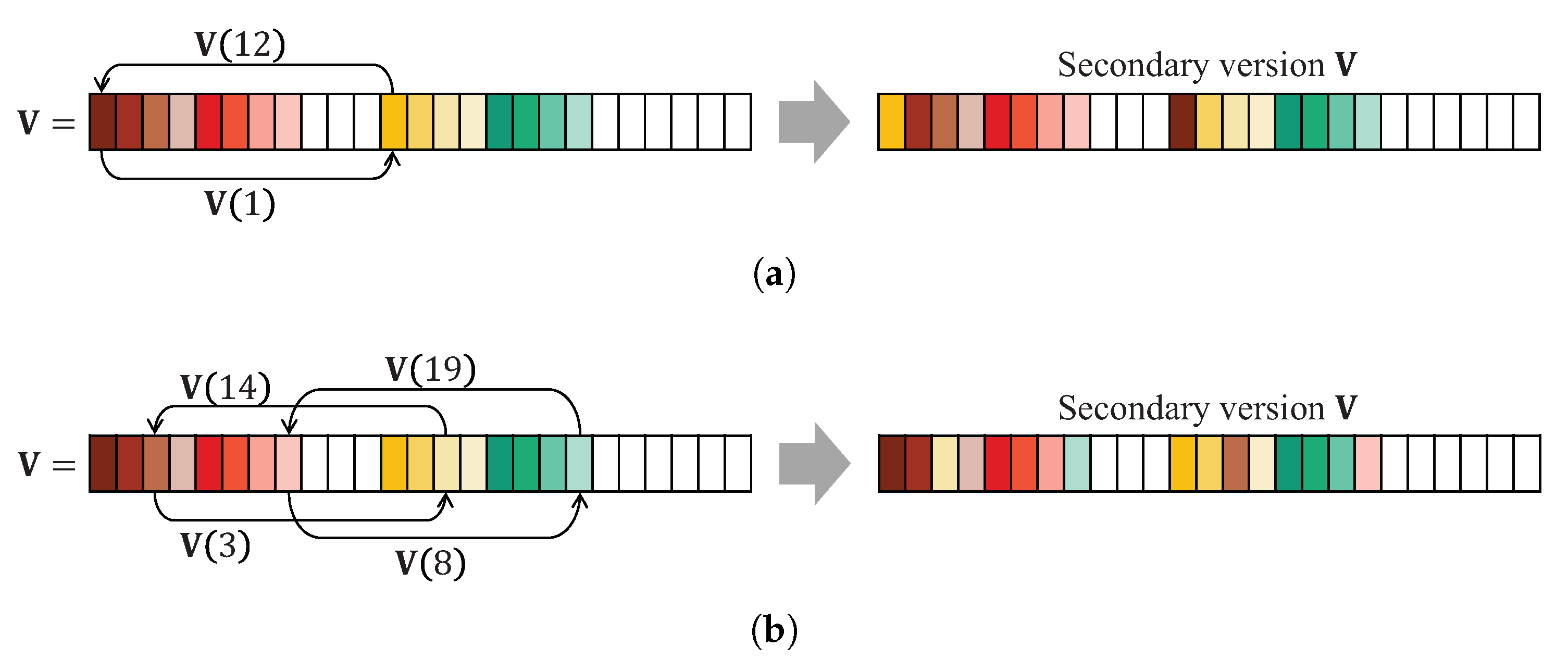
In the proposed method, several secondary versions are generated from $\mathbf{V}$ by exchanging its elements corresponding to the symmetric limbs. In addition, this exchange process is performed with different combinations of pairs. For example, suppose that the exchange is performed for five out of the eight pairs. In addition, let $C(p,q)$ be the number of q-combinations from a given set of p elements. Then, 56 combinations can be generated from the selected five out of eight pairs (i.e., $C(8,5)=8!/(5!3!)=56$, where $r!$ denotes the factorial of r). Therefore, because the number of pairs of symmetric limbs is eight, the number of q-combinations for all $q\in \{1,2,\cdots ,7,8\}$ is ${\sum }_{q=1}^{8}C(8,q)=2^8-1=255$.

In each of the 255 combinations above, q distinct index numbers represent the pairs selected from the eight pairs. In the proposed method, based on these index numbers, the elements of $\mathbf{V}$ that need to be exchanged are selected. For example, suppose that Pair 1 is selected out of the eight pairs (i.e., $q=1$) for exchange. The first pair (Limb #1, Limb #12) is selected. The secondary version $\mathbf{V}$ is then generated as shown in Figure 8a. For another example, two numbers indexed 3 and 8 are selected. The pairs (Limb #3, Limb #14) and (Limb #8, Limb #19) are then constructed. The secondary version $\mathbf{V}$ is then generated by exchanging $\mathbf{V}$(3) and $\mathbf{V}$(14), and $\mathbf{V}$(8) and $\mathbf{V}$(19), as shown in Figure 8b.

Therefore, for $q\in \{1,2,\cdots ,7,8\}$, the total number in the secondary version $\mathbf{V}$ is ${\sum }_{q=1}^{8}C(8,q)=255$. We present its pseudocode in Algorithm 1, where $\mathbf{S}$ is the secondary version $\mathbf{V}$ and its dimension is $255\times 25$. According to the pseudocode, the total number of anthropometric feature vectors is increased up to 256 times (including the original vector) as shown in Figure 9.

Algorithm 1 Pseudocode of the proposed data augmentation method

Input:$1\times 25$-dimensional feature vector of $\mathbf{V}$

Output:$255\times 25$-dimensional matrix of $\mathbf{S}$

1: count = 1; 2: $\mathbf{S}$ = zeros(255, 25); 3: for q = 1:1:8 do 4:   comb = nchoosek(1:1:8, q); 5:   for b = 1:1:size(comb, 1) do 6:     $\mathbf{S}$(count, :) = $\mathbf{V}$; 7:     temp1 = $\mathbf{V}$(comb(b, :)); 8:     temp2 = $\mathbf{V}$(comb(b, :) + 11); 9:     $\mathbf{S}$(count, comb(b, :)) = temp2; 10:     $\mathbf{S}$(count, comb(b, :) + 11) = temp1; 11:     count = count + 1; 12:   end for 13: end for

5.2. Deep Neural Network for Person Identification

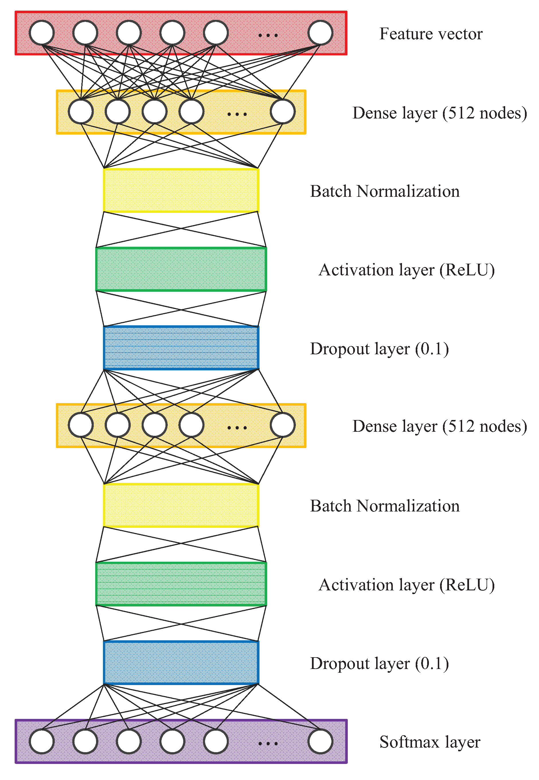
Figure 10 illustrates the architecture of the DNN. The DNN accepts the input of the anthropometric feature vectors. The dense layer, which has 512 fully connected dense nodes, is added after the input layer. The output of the dense layer can be represented by (12) as follows:

$$\begin{array}{c}\hfill {\mathbf{O}}_1=\mathbf{V}·\mathbf{W}\end{array}$$

(12)

where $\mathbf{W}$ is a $25\times 512$ dimensional weight matrix. Let B be the batch selected at each epoch and S be the size of B. The dimension of ${\mathbf{O}}_1$ then becomes $S\times 512$.

To prevent overfitting and improve the speed, performance, and stability, we added a batch normalization layer after the dense layer. Hence, at the batch normalization layer, the mean of B can be calculated by (13) as follows:

$$\begin{array}{c}\hfill {\mathbf{\mu }}_B=\frac{1}{S}\sum _{s=1}^S{\mathbf{O}}_1\left(s\right),\end{array}$$

(13)

where ${\mathbf{O}}_1\left(s\right)$ is the $s\mathrm{th}$ row vector of ${\mathbf{O}}_1$ and the dimension of ${\mathbf{\mu }}_B$ is $1\times 512$. In addition, using ${\mathbf{\mu }}_B$ in (13), the variance of B is

$$\begin{array}{c}\hfill {\mathbf{\sigma }}_B^2=\frac{1}{S}\sum _{s=1}^S{\left\{{\mathbf{O}}_1\left(s\right)-{\mathbf{\mu }}_B\right\}}^2\end{array}$$

(14)

where ${\mathbf{\sigma }}_B^2$ has the dimension of $1\times 512$.

Let ${\mathbf{O}}_1(s,v)$ be the $v\mathrm{th}$ element of ${\mathbf{O}}_1\left(s\right)$, ${\mathbf{\mu }}_B\left(v\right)$ be the $v\mathrm{th}$ element of ${\mathbf{\mu }}_B$, and ${\mathbf{\sigma }}_B^2\left(v\right)$ be the $v\mathrm{th}$ element of ${\mathbf{\sigma }}_B^2$. Then, the normalized ${\mathbf{O}}_1(s,v)$ becomes

$$\begin{array}{c}\hfill {\tilde{\mathbf{O}}}_1(s,v)=\frac{{\mathbf{O}}_1(s,v)-{\mathbf{\mu }}_B\left(v\right)}{\sqrt{{\mathbf{\sigma }}_B^2\left(v\right)+ϵ}}\end{array}$$

(15)

where $s\in \{1,2,\cdots ,S-1,S\}$, $v\in \{1,2,\cdots ,511,512\}$ and $ϵ$ is a small constant value added for numerical stability. In this study, the value of $ϵ$ is set to 0.001.

Using ${\tilde{\mathbf{O}}}_1(s,v)$ in (15), the output of the batch normalization layer is

$$\begin{array}{c}\hfill {\mathbf{O}}_2(s,v)=\gamma \left(v\right)·{\tilde{\mathbf{O}}}_1(s,v)+\beta \left(v\right),\end{array}$$

(16)

where the parameters $\gamma \left(v\right)$ and $\beta \left(v\right)$ are learned during the optimization process of the training phase.

In the DNN, the activation layer is added after the batch normalization layer. At the activation layer, we used the rectified linear unit (ReLU) activation function proposed in [46] to add non-linearity to the DNN. Therefore, the output of the activation layer is

$$\begin{array}{c}\hfill {\mathbf{O}}_3(s,v)=max({\mathbf{O}}_2(s,v),0),\end{array}$$

(17)

where $max(a,0)$ is the function that returns “a” for $a>0$ and 0 otherwise.

After the activation layer, a dropout layer is added. During the training phase, at the dropout layer, input units are randomly dropped out at specified rates. In the DNN, the dropout rate is set to 0.1. The second dense layer, batch normalization layer, activation layer, and dropout layer are then successively added as described above. In addition, the number of dense nodes of the second dense layer is the same as that of the first dense layer as shown in Figure 10. At the second activation layer, the ReLU activation function is used. The dropout rate of 0.1 is set in the second dropout layer.

At the end of the DNN, the softmax layer is added to classify the labels for each person. In this layer, the softmax function is used as the activation function. Therefore, the activation values from the softmax layer are normalized by:

$$\begin{array}{c}\hfill {\tilde{y}}_{\theta }=\frac{\exp \left(y_{\theta }\right)}{{\sum }_{\vartheta =1}^{\mathsf{\Theta }}\exp \left(y_{\vartheta }\right)},\forall \theta \in \{1,2,\cdots ,\mathsf{\Theta }-1,\mathsf{\Theta }\}\end{array}$$

(18)

where $\exp (·)$ is the exponential function and $\theta$ is the label for the $\theta \mathrm{th}$ person. In addition, ${\tilde{y}}_{\theta }$ and $y_{\theta }$ are the normalized and unnormalized activation values, respectively. If the person identification dataset contains $\mathsf{\Theta }$ subjects in total, the total number of labels becomes $\mathsf{\Theta }$. In addition, the softmax layer outputs a $1\times \mathsf{\Theta }$-dimensional vector where the $\theta \mathrm{th}$ value of the vector is ${\tilde{y}}_{\theta }$. To train the DNN, we apply the sparse categorical cross entropy loss function to the objective function.

6. Experimental Evaluation and Results

6.1. Dataset and Evaluation Protocol

We evaluated the proposed method on the existing publicly available person identification dataset, called Andersson’s dataset [23,24,25]. To the best of our knowledge, this dataset contains the largest number of subjects, compared to other publicly available datasets. For this reason, this dataset has been widely used to test person identification methods. It contains 164 subjects in total, with five sequences for each subject. However, there are only three or four sequences for the following four subjects: “Person002,” “Person015,” “Person158,” and “Person164.” We eliminated these four subjects from the dataset. In addition, there are six sequences for the following seven subjects: “Person003,” “Person034,” “Person036,” “Person052,” “Person053,” “Person074,” and “Person096.” Observing the six sequences for each subject, we decided to eliminate the noisiest sequence. Consequently, the $4\mathrm{th}$ sequence of “Person003,” $1\mathrm{st}$ sequence of “Person034,” $3\mathrm{rd}$ sequence of “Person036,” $5\mathrm{th}$ sequence of “Person052,” $5\mathrm{th}$ sequence of “Person053,” $3\mathrm{rd}$ sequence of “Person074,” and $6\mathrm{th}$ sequence of “Person096” were eliminated from the dataset. As a result, the dataset contains a total of 800 $(=160\mathrm{subjects}\times 5\mathrm{sequences}\mathrm{per}\mathrm{subject})$ sequences.

We used the 5-fold cross-validation to evaluate the performance of each method. In each cross-validation, for each subject, four sequences were selected from a total of five. The selected 640 sequences $(=160\mathrm{subjects}\times 4\mathrm{sequences}\mathrm{per}\mathrm{subject})$ were used for the training dataset. In addition, the remaining 160 $(=800-640)$ sequences were used for the testing dataset.

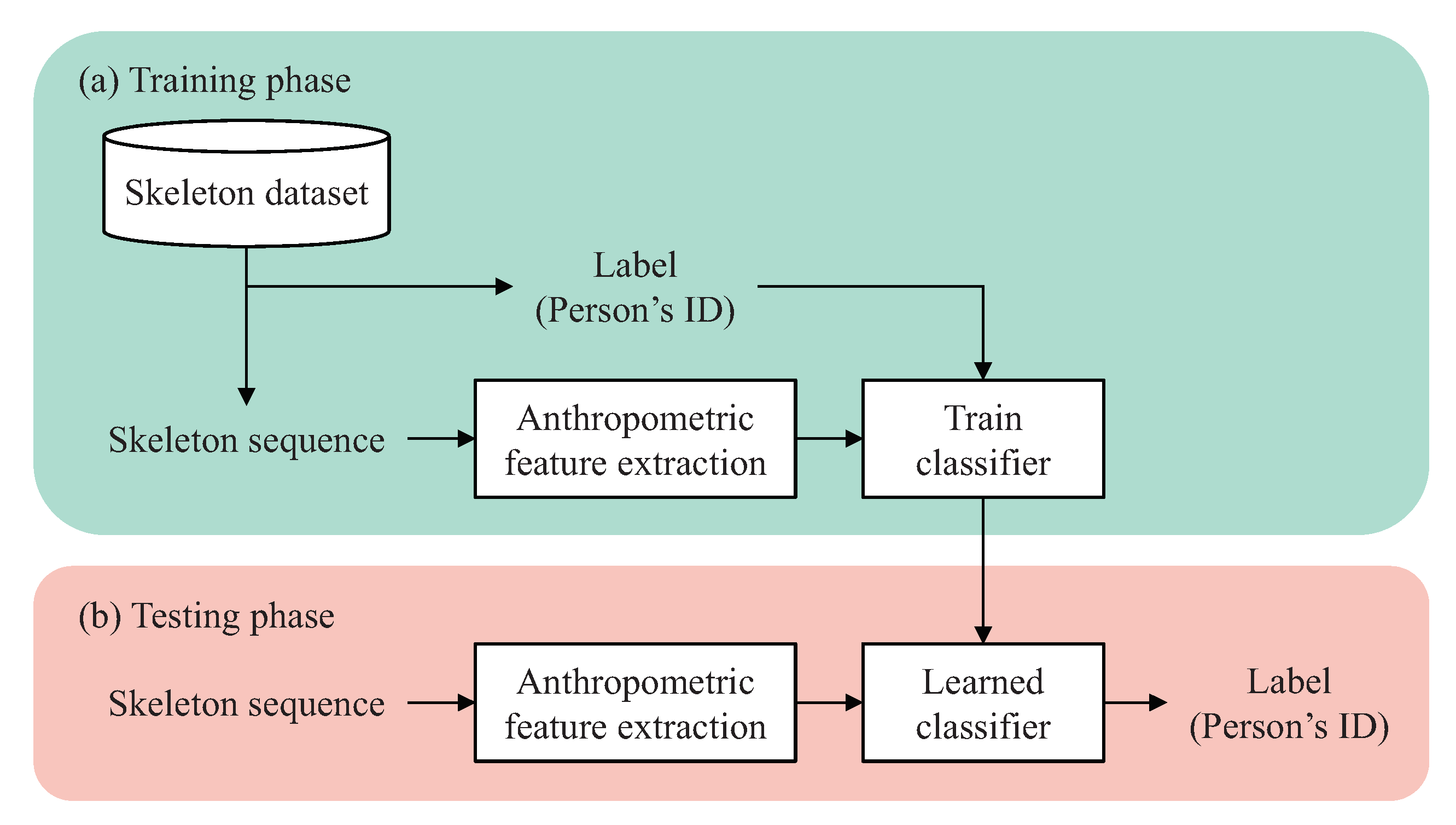
6.2. Four Benchmark Methods

For performance comparison, we implemented four person identification methods: (1) C-SVM, (2) nu-SVM, (3) k-NN, and (4) MLP. Figure 11 shows the block diagram for the training and testing phases of the four methods. Each classifier was trained to learn the person identification task. The anthropometric features, as described in Section 4, were extracted from the input skeleton sequence. They were inputted to each classifier in a form of vector. The four methods are detailed as follows:

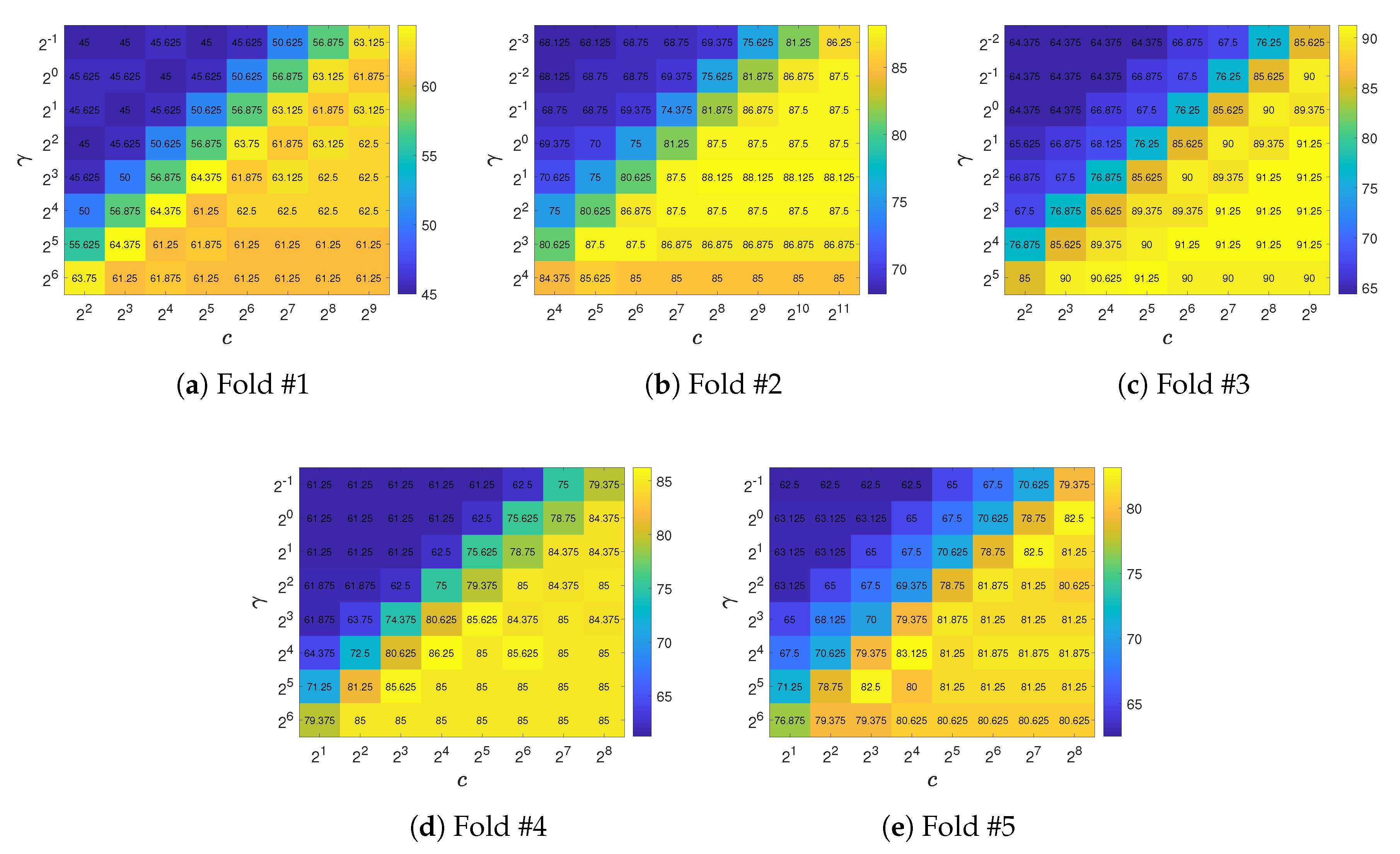
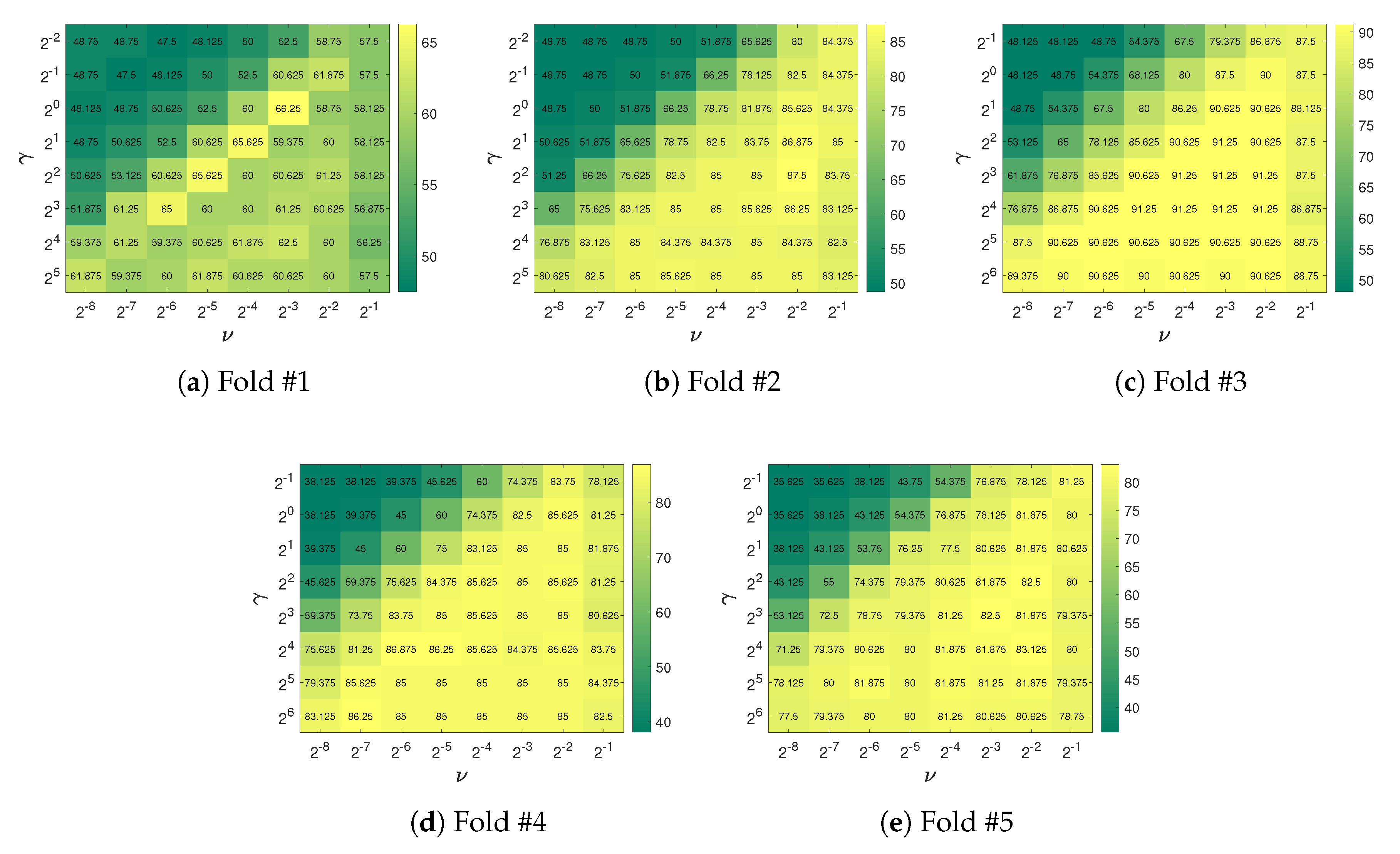
• C-SVM and nu-SVM: To implement C-SVM and nu-SVM that support multi-class classification, we used LIBSVM—an open-source library for SVMs [47]. According to the recommendation in [48], we used the radial basis function (RBF) kernel for C-SVM and nu-SVM. C-SVM has a cost parameter, denoted c, whose value ranges from 0 to ∞. The nu-SVM method has a regularization parameter, denoted g, with a value range $\left[0,1\right]$. The RBF kernel has a gamma parameter, denoted $\gamma$. The grid search method was used to find the best parameter combination for both C-SVM and nu-SVM.
• k-NN: According to the results of the previous studies [22,23,24,25], k-NN achieved the best performance in the task of person identification. To implement k-NN, we used the MATLAB function fitcknn. To determine the best hyperparameter configuration, we performed hyperparameter optimization supported in the function fitcknn.
• MLP: According to the results of the previous studies [22,23,24,25], MLP showed the worst performance in the task of person identification. In [22], MLP had 10 hidden units. In [23], the number of hidden units was 20. Conversely, in [24,25], MLP, which had 40 hidden units, was used. For performance comparison, we implemented the three MLPs using TensorFlow [49]. However, as mentioned in Section 3, in the experiments, we observed that the training set accuracy of each MLP was lower than 10% when each MLP comprised only a single hidden layer. Therefore, to overcome this issue and to improve the training set accuracy, the batch normalization layer, activation layer, and dropout layer were successively added after the hidden layer of each MLP. For simplicity, we called the three MLPs: MLP-10, MLP-20, and MLP-40, respectively. Here, the suffix number denotes the number of hidden units in the hidden layer.

6.3. Results and Comparisons

In each cross-validation, the grid search method was used to find the best parameters c and $\gamma$ for C-SVM. Figure 12 shows the grid search results for C-SVM over the 5-fold cross-validation. C-SVM achieved an average accuracy of 82.625% over the 5-fold cross-validation. To find the best values of g and $\gamma$ parameters for nu-SVM, the grid search method was used in each cross-validation. Figure 13 shows the grid search results for nu-SVM over the 5-fold cross-validation; nu-SVM achieved an average accuracy of 83%.

Table 3. Hyperparameter optimization results for k-NN over 5-fold cross-validation.

Fold #	Hyperparameters
	k	Distance Metric	Distance Weighting Function	Exponent	Standardize	Accuracy (%)
1	1	euclidean	inverse	-	true	73.125
2	3	cityblock	squaredinverse	-	true	88.750
3	3	minkowski	squaredinverse	0.8615	true	93.750
4	1	minkowski	equal	0.8335	true	93.750
5	2	minkowski	squaredinverse	2.1445	true	83.125

lists the hyperparameter optimization results for k-NN over the 5-fold cross-validation. As shown in the table, the optimal hyperparameters found at each cross-validation of each dataset were mutually different. In the table, the person identification accuracy of each k-NN over the 5-fold cross-validation is also listed. The results in the table show that k-NN achieved an average accuracy of 86.5%.

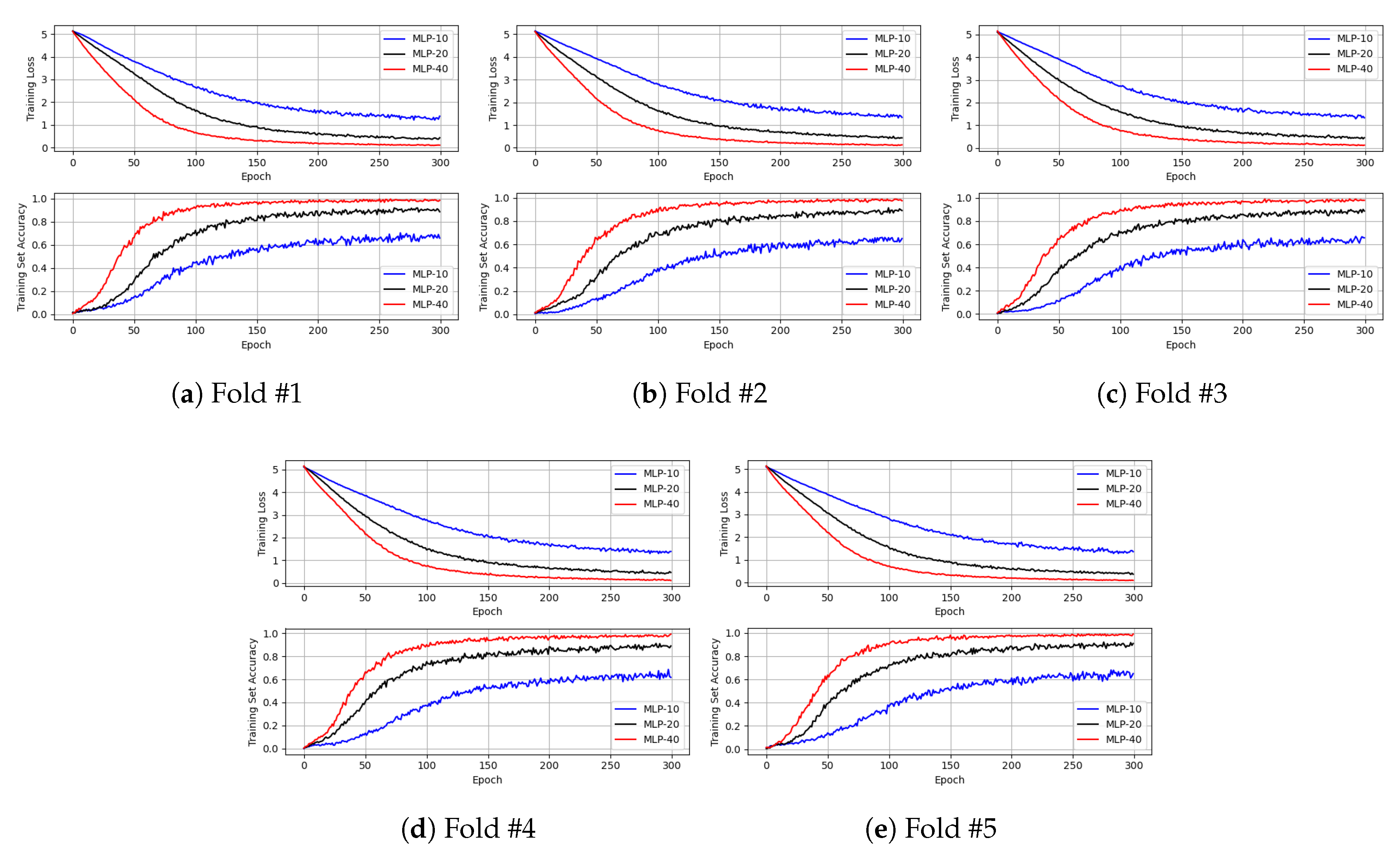
Figure 14 shows the training loss and training set accuracy of each MLP over 5-fold cross-validation. In the experiments, the batch size was set to 64; the Adam optimizer proposed in [50] was used for the training; an ReLU activation function was used; the dropout rate was set to 0.1. As shown in this figure, the convergence speed of the training loss of MLP-40 was the fastest among the MLP-based methods. In addition, the training set accuracy of MLP-40 outperforms that of MLP-10 and MLP-20. As shown in Figure 14, MLP-40 achieves a training set accuracy of approximately 100%, whereas MLP-10 and MLP-20 achieve an accuracy of approximately 60% and 90%, respectively. In particular, in the experiments, it is observed that the training set accuracy of each MLP is lower than 10% when the batch normalization layer is not added. From the results, the batch normalization could be seen to effectively improve the person identification accuracy of MLP-based methods. For this reason, the batch normalization layer was added after the hidden layer of each MLP.

Table 4. Testing set accuracy (%) of each MLP over 5-fold cross-validation.

Fold #	MLP
	MLP-10	MLP-20	MLP-40
1	46.250	47.500	51.250
2	56.880	76.250	76.880
3	72.500	80.000	81.250
4	50.370	74.370	77.500
5	60.620	69.380	76.880
Avg.	57.324	69.500	72.752

shows the testing set accuracy of each MLP over the 5-fold cross-validation. As shown in this table, on the testing datasets, MLP-40 achieves the best average accuracy of 72.752%. However, compared with the training set accuracy of MLP-40 in Figure 14, the accuracy of MLP-40 is significantly lower for the testing datasets. The accuracy of MLP-10 and MLP-20 are also lower for the testing datasets, compared with the results in Figure 14. The results show that overfitting occurred in the training phase of each MLP.

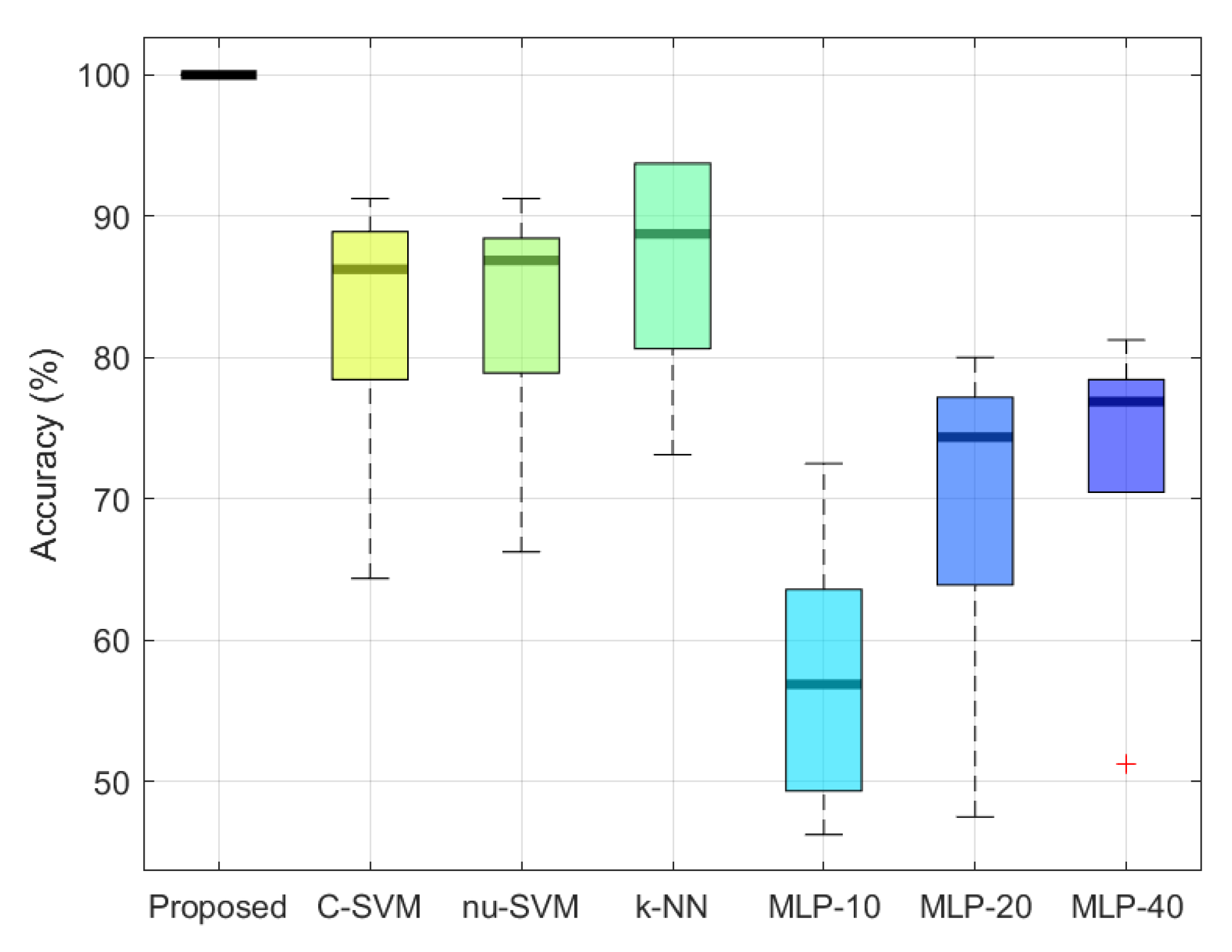
Figure 15 shows the accuracy of each method over the 5-fold cross-validation. In the figure, the proposed DNN of using the augmented training dataset is denoted “Proposed.” In the training phase of each cross-validation, the proposed data augmentation method was applied to 640 anthropometric feature vectors $\mathbf{V}$. Resulting from the application of the proposed data augmentation method, the total number of $\mathbf{V}$ became 163,840 $(=640\times 256)$. Using this augmented training dataset, the proposed DNN could be trained without overfitting. During the training phase, the batch size was set to 1000 and the Adam optimizer was used. As a result, as shown in Figure 15, the proposed DNN achieved 100% person identification accuracy for all cross-validation folds.

The average accuracy of each method is listed in

Table 5. Average accuracy (%) comparison.

Method	Accuracy
C-SVM	82.625
nu-SVM	83.000
k-NN	86.500
MLP-10	57.324
MLP-20	69.500
MLP-40	72.752
MLP-10 + Proposed DA	75.528
MLP-20 + Proposed DA	93.752
MLP-40 + Proposed DA	98.372
Proposed DNN + Proposed DA	100.000

. Among the benchmark methods, k-NN achieves the best average accuracy of 86.5%, whereas MLP-10 exhibits the worst with 57.324%. The person identification accuracy of the proposed method (“Proposed DNN+Proposed DA”) is greater than that of k-NN by 23.5%. Moreover, in the experiments shown in the table, to validate the effectiveness of the proposed data augmentation method, we trained MLP-10, MLP-20, and MLP-40 using the augmented training dataset and denoted them as “MLP-10+Proposed DA,” “MLP-20+Proposed DA,” and “MLP-20+Proposed DA.” As shown in the table, the proposed data augmentation method improves the person identification accuracy of “MLP-10+Proposed DA,” “MLP-20+Proposed DA,” and “MLP-30+Proposed DA” compared to those of MLP-10, MLP-20, and MLP-40. For MLP-40, the average accuracy is improved by 25.62%. For MLP-20, it is improved by 24.252%. In addition, for MLP-10, it is improved by 18.204%. Therefore, from the results, the proposed data augmentation method is seen to improve the performance of neural network models by preventing overfitting. In addition, the proposed DNN achieves the best performance among all the methods.

Table 6. Performance comparison between the proposed and benchmark data augmentation methods.

Method	Fold #1	Fold #2	Fold #3	Fold #4	Fold #5	Avg.
Proposed DA	100.00	100.00	100.00	100.00	100.00	100.00
Benchmark DA #1	52.50	59.38	62.50	52.50	68.12	59.00
Benchmark DA #2	68.12	63.75	86.87	61.25	73.12	70.62
Benchmark DA #3	63.13	88.75	75.63	83.75	77.50	77.75
Benchmark DA #4	64.38	87.50	90.00	84.38	76.25	80.50

shows the identification accuracy of the proposed and benchmarked data augmentation methods. For the benchmark, the skeleton sequence is divided into several segments with an equal length. In the experiments of the table, we divided the original sequence with five different segment lengths. From the frame division process, 15 segments corresponding to each length are generated as one for F, two for $F/2$, three for $F/3$, four for $F/4$, and five for $F/5$. Then, the anthropometric feature vectors are calculated for each segment. By doing this, the feature vectors used for training of the DNN can be augmented in the benchmark method. In “Benchmark DA #1,” the anthropometric feature vectors were calculated for 3 segments (one for F and two for $F/2$). Therefore, the total number of training datasets becomes 1960 $(=3\times 640)$. In “Benchmark DA #2,” the feature vectors were calculated for 6 segments (one for F, two for $F/2$, and three for $F/3$), and the total number of training datasets becomes 3840 $(=6\times 640)$. In “Benchmark DA #3,” the feature vectors were calculated for 10 segments (one for F, two for $F/2$, three for $F/3$, four for $F/4$), and the total number of training datasets becomes 6400 $(=10\times 640)$. In “Benchmark DA #4,” the feature vectors were calculated for 15 segments (one for F, two for $F/2$, three for $F/3$, four for $F/4$, and five for $F/5$), and the total number of training datasets becomes 9600 $(=15\times 640)$. As shown in the table, the performance of the proposed data augmentation method outperforms the other benchmarked method. Among the benchmarks, “Benchmark DA #4” performed the best because the number of augmented training datasets was greater than those of the others.

Table 7. Performance comparison of DNN according to the number of dense layers and the number of dense nodes per layer.

Parameter		Number of Dense Layers (${\mathit{D}}_{\mathit{L}}$)
		1	2	3	4	5
Number of dense nodes per layer ($D_N$)	2	14.876	9.372	8.998	8.124	5.874
	4	44.126	28.876	27.624	21.498	16.378
	8	65.502	56.626	49.998	47.248	46.750
	16	84.674	82.548	81.500	78.752	75.626
	32	95.462	94.348	91.370	88.200	85.374
	64	97.498	98.700	94.670	92.266	89.736
	128	97.983	99.120	98.316	96.189	94.586
	256	98.500	99.874	99.374	98.626	97.876
	512	99.248	100.000	100.000	100.000	100.000

shows the average accuracy of the DNN according to the number of dense layers and the number of dense nodes per layer. It was a big issue to determine how many dense layers and dense nodes per layer are needed to guarantee the accuracy of the DNN. For this purpose, we used the grid search method. For explanation, let $D_L$ be the number of dense layers of the DNN and $D_N$ be the number of dense nodes per layer. To find the best parameter configuration, in the experiments, $D_L$ was set to the range of $\{1,2,3,4,5\}$ and $D_N$ was set to the range of $\{2^1,2^2,\cdots ,2^8,2^9\}$. As shown in the table, as $D_N$ increases, the average accuracy of the DNN increases. In other words, if $D_N$ is not sufficiently large, the accuracy of the DNN was not guaranteed. In the experiments, when $D_N=512$ and $D_L\in \{2,3,4,5\}$, the DNN achieved $100\%$ accuracy. Based on the results in the table, we used the DNN consisting of 2 dense layers with 512 dense nodes per layer.

To find the best activation function of the DNN, we evaluated the average accuracy of the DNN according to the activation function: the ReLU, sigmoid, softmax, softplus, softsign, tanh, scaled exponential linear unit (SELU) [51], exponential linear unit (ELU) [52], and exponential activation functions.

Table 8. Performance comparison of DNN according to the activation functions.

Activation Function	ReLU	Sigmoid	Softmax	Softplus	Softsign	Tanh	SELU	ELU	Exponential
Average accuracy	100	100	20.88	100	100	99.87	100	100	67.34

shows the evaluation results. In the experiments of the table, the DNN consisting of 2 dense layers with 512 dense nodes per layer was used. As shown in the table, for the ReLU, sigmoid, softplus, softsign, SELU, and ELU activation functions, the DNN achieved 100% accuracy. On the other hand, for the softmax, tanh, and exponential action functions, the accuracy of the DNN was not guaranteed. Therefore, based on the results in the table, we proposed to use one among the six activation functions. In this study, we used the ReLU activation function.

To find the best dropout rate of the DNN, we evaluated the average accuracy of the DNN according to the dropout rate.

Table 9. Performance comparison of DNN according to the dropout rate.

Dropout rate	0.0	0.1	0.2	0.3	0.4
Average accuracy	100	100	96.126	76.872	53.872

shows the evaluation results. In the experiments of the figure, the DNN consisting of 2 dense layers with 512 dense nodes per layer was used. In addition, the ReLU activation function was used in each activation layer of the DNN. The dropout rate was set to range of $\{0.0,0.1,0.2,0.3,0.4\}$. In the experiments, for all the dropout rates, the DNN achieved a training set accuracy of 100%. However, as shown in the table, as the dropout rate increases, the average testing set accuracy decreases. Only when the dropout rate was set to either 0.0 or 0.1, the DNN achieved a testing set accuracy of 100%. Therefore, based on the results in the table, we proposed to use one between the dropout rates of 0.0 and 0.1. In this study, we used the dropout rate of 0.1.

7. Discussion

The skeleton model estimated from RGB image (or depth image) generally contains the noise and error (referred as the uncertainty) introduced from key point/joint detection methods [53]. This uncertainty makes the differences between the anthropometric features extracted from the symmetric parts of the human body (i.e., one is extracted from the right side and the other is extracted from the left side). By exchanging these features, the proposed data augmentation method generates the new anthropometric feature vectors. However, with the advancement in pose estimation techniques, if the uncertainty is significantly reduced and the anthropometric features extracted from the left (or right) side of the human body become exactly the same with the corresponding right (or left) features, the feature vectors augmented by the method become all the same. Therefore, in this case, the effectiveness and usefulness of the proposed augmentation method can be limited.

8. Conclusions

In this study, we proposed a skeleton-based person identification method using DNN. The anthropometric features extracted from the human skeleton sequence were used as input to the DNN. However, when training the DNN on the existing public dataset, overfitting occurred during the training phase. As a result, the DNN could not achieve the desired testing set accuracy. To prevent overfitting and improve the testing set accuracy, we proposed a novel data augmentation method. In the method, the augmented vectors were generated by exchanging the anthropometric features extracted from the left side of the human body to the corresponding features extracted from the right side. Using this method, the total number of anthropometric feature vectors was increased by 256 times. Experimental results demonstrated that the proposed DNN identified individuals with 100% accuracy when the DNN was trained on the augmented training dataset.

References

1. Jain, A.K.; Ross, A.; Pankanti, S. Biometrics: A tool for information security. IEEE Trans. Inf. Forensics Secur. 2006, 1, 125–143. [Google Scholar] [CrossRef] [Green Version]
2. Eastwood, S.C.; Shmerko, V.P.; Yanushkevich, S.N.; Drahansky, M.; Gorodnichy, D.O. Biometric-enabled authentication machines: A survey of open-set real-world applications. IEEE Trans. Hum.-Mach. Syst. 2016, 46, 231–242. [Google Scholar] [CrossRef]
3. Park, K.; Park, J.; Lee, J. An IoT system for remote monitoring of patients at home. Appl. Sci. 2017, 7, 260. [Google Scholar] [CrossRef] [Green Version]
4. Zhang, Y.; Mu, Z.; Yuan, L.; Zeng, H.; Chen, L. 3D ear normalization and recognition based on local surface variation. Appl. Sci. 2017, 7, 104. [Google Scholar] [CrossRef] [Green Version]
5. Shnain, N.A.; Hussain, Z.M.; Lu, S.F. A feature-based structural measure: An image similarity measure for face recognition. Appl. Sci. 2017, 7, 786. [Google Scholar] [CrossRef] [Green Version]
6. Chen, J.; Zhao, H.; Cao, Z.; Guo, F.; Pang, L. A Customized Semantic Segmentation Network for the Fingerprint Singular Point Detection. Appl. Sci. 2020, 10, 3868. [Google Scholar] [CrossRef]
7. Li, C.; Min, X.; Sun, S.; Lin, W.; Tang, Z. DeepGait: A learning deep convolutional representation for view-invariant gait recognition using joint Bayesian. Appl. Sci. 2017, 7, 210. [Google Scholar] [CrossRef]
8. Tobji, R.; Di, W.; Ayoub, N. FMnet: Iris Segmentation and Recognition by Using Fully and Multi-Scale CNN for Biometric Security. Appl. Sci. 2019, 9, 2042. [Google Scholar] [CrossRef] [Green Version]
9. Izadpanahkakhk, M.; Razavi, S.M.; Taghipour-Gorjikolaie, M.; Zahiri, S.H.; Uncini, A. Deep region of interest and feature extraction models for palmprint verification using convolutional neural networks transfer learning. Appl. Sci. 2018, 8, 1210. [Google Scholar] [CrossRef] [Green Version]
10. Galka, J.; Masior, M.; Salasa, M. Voice authentication embedded solution for secured access control. IEEE Trans. Consum. Electron. 2014, 60, 653–661. [Google Scholar] [CrossRef]
11. Collins, R.T.; Gross, R.; Shi, J. Silhouette-based human identification from body shape and gait. In Proceedings of the IEEE International Conference on Automatic Face and Gesture Recognition (FG), Washington, DC, USA, 21 May 2002; pp. 366–371. [Google Scholar]
12. Wang, L.; Tan, T.; Ning, H.; Hu, W. Silhouette analysis-based gait recognition for human identification. IEEE Trans. Pattern Anal. Mach. Intell. 2003, 25, 1505–1518. [Google Scholar] [CrossRef] [Green Version]
13. Liu, Z.; Malave, L.; Sarkar, S. Studies on silhouette quality and gait recognition. In Proceedings of the IEEE Computer Society Conference on Computer Vision and Pattern Recognition (CVPR), Washington, DC, USA, 27 June–2 July 2004; pp. 704–711. [Google Scholar]
14. Liu, Z.; Sarkar, S. Simplest representation yet for gait recognition: Averaged silhouette. In Proceedings of the IEEE International Conference on Pattern Recognition (ICPR), Cambridge, UK, 26 August 2004; pp. 211–214. [Google Scholar]
15. Liu, Z.; Sarkar, S. Effect of silhouette quality on hard problems in gait recognition. IEEE Trans. Syst. Man Cybern. Part B (Cybern.) 2005, 35, 170–183. [Google Scholar] [CrossRef] [PubMed] [Green Version]
16. Shotton, J.; Fitzgibbon, A.; Cook, M.; Sharp, T.; Finocchio, M.; Moore, R.; Kipman, A.; Blake, A. Real-time human pose recognition in parts from single depth images. In Proceedings of the IEEE Computer Society Conference on Computer Vision and Pattern Recognition (CVPR), Colorado Springs, CO, USA, 20–25 June 2011; pp. 1297–1304. [Google Scholar]
17. Kwon, B.; Kim, D.; Kim, J.; Lee, I.; Kim, J.; Oh, H.; Kim, H.; Lee, S. Implementation of human action recognition system using multiple Kinect sensors. In Proceedings of the 16th Pacific Rim Conference on Multimedia (PCM), Gwangju, Korea, 16–18 September 2015; pp. 334–343. [Google Scholar]
18. Kwon, B.; Kim, J.; Lee, S. An enhanced multi-view human action recognition system for virtual training simulator. In Proceedings of the Asia–Pacific Signal and Information Processing Association Annual Summit Conference (APSIPA ASC), Jeju, Korea, 13–16 December 2016; pp. 1–4. [Google Scholar]
19. Kwon, B.; Kim, J.; Lee, K.; Lee, Y.K.; Park, S.; Lee, S. Implementation of a virtual training simulator based on 360° multi-view human action recognition. IEEE Access 2017, 5, 12496–12511. [Google Scholar] [CrossRef]
20. Munsell, B.C.; Temlyakov, A.; Qu, C.; Wang, S. Person identification using full-body motion and anthropometric biometrics from Kinect videos. In Proceedings of the European Conference on Computer Vision (ECCV), Florence, Italy, 7–13 October 2012; pp. 91–100. [Google Scholar]
21. Wu, J.; Konrad, J.; Ishwar, P. Dynamic time warping for gesture-based user identification and authentication with Kinect. In Proceedings of the IEEE International Conference on Acoustics, Speech and Signal Processing (ICASSP), Vancouver, BC, Canada, 26–31 May 2013; pp. 2371–2375. [Google Scholar]
22. Araujo, R.; Graña, G.; Andersson, V. Towards skeleton biometric identification using the Microsoft Kinect sensor. In Proceedings of the 28th Symposium on Applied Computing (SAC), Coimbra, Portugal, 18–22 March 2013; pp. 21–26. [Google Scholar]
23. Andersson, V.; Dutra, R.; Araujo, R. Anthropometric and human gait identification using skeleton data from Kinect sensor. In Proceedings of the 29th Symposium on Applied Computing (SAC), Gyeongju, Korea, 24–28 March 2014; pp. 60–61. [Google Scholar]
24. Andersson, V.; Araujo, R. Full body person identification using the Kinect sensor. In Proceedings of the 26th IEEE International Conference on Tools with Artificial Intelligence (ICTAI), Limassol, Cyprus, 10–12 November 2014; pp. 627–633. [Google Scholar]
25. Andersson, V.; Araujo, R. Person identification using anthropometric and gait data from Kinect sensor. In Proceedings of the 29th Association for the Advancement of Artificial Intelligence (AAAI) Conference on Artificial Intelligence, Austin, TX, USA, 25–30 January 2015; pp. 425–431. [Google Scholar]
26. Yang, K.; Dou, Y.; Lv, S.; Zhang, F.; Lv, Q. Relative distance features for gait recognition with Kinect. J. Vis. Commun. Image Represent. 2016, 39, 209–217. [Google Scholar] [CrossRef] [Green Version]
27. Sun, J.; Wang, Y.; Li, J.; Wan, W.; Cheng, D.; Zhang, H. View-invariant gait recognition based on Kinect skeleton feature. Multimed. Tools Appl. 2018, 77, 24909–24935. [Google Scholar] [CrossRef]
28. Huitzil, I.; Dranca, L.; Bernad, J.; Bobillo, F. Gait recognition using fuzzy ontologies and Kinect sensor data. Int. J. Approx. Reason. 2019, 113, 354–371. [Google Scholar] [CrossRef]
29. Donati, L.; Iotti, E.; Mordonini, G.; Prati, A. Fashion Product Classification through Deep Learning and Computer Vision. Appl. Sci. 2019, 9, 1385. [Google Scholar] [CrossRef] [Green Version]
30. Young, T.; Hazarika, D.; Poria, S.; Cambria, E. Recent trends in deep learning based natural language processing. IEEE Comput. Intell. Mag. 2018, 13, 55–75. [Google Scholar] [CrossRef]
31. Song, H.; Kwon, B.; Lee, S.; Lee, S. Dictionary based compression type classification using a CNN architecture. In Proceedings of the Asia–Pacific Signal and Information Processing Association Annual Summit Conference (APSIPA ASC), Lanzhou, China, 18–21 November 2019; pp. 245–248. [Google Scholar]
32. Kwon, B.; Song, H.; Lee, S. Accurate blind Lempel-Ziv-77 parameter estimation via 1-D to 2-D data conversion over convolutional neural network. IEEE Access 2020, 8, 43965–43979. [Google Scholar] [CrossRef]
33. Nguyen, N.D.; Nguyen, T.; Nahavandi, S. System design perspective for human-level agents using deep reinforcement learning: A survey. IEEE Access 2017, 5, 27091–27102. [Google Scholar] [CrossRef]
34. Menger, V.; Scheepers, F.; Spruit, M. Comparing deep learning and classical machine learning approaches for predicting inpatient violence incidents from clinical text. Appl. Sci. 2018, 8, 981. [Google Scholar] [CrossRef] [Green Version]
35. Kulyukin, V.; Mukherjee, S.; Amlathe, P. Toward audio beehive monitoring: Deep learning vs. standard machine learning in classifying beehive audio samples. Appl. Sci. 2018, 8, 1573. [Google Scholar] [CrossRef] [Green Version]
36. Gu, Y.; Wang, Y.; Li, Y. A survey on deep learning-driven remote sensing image scene understanding: Scene classification, scene retrieval and scene-guided object detection. Appl. Sci. 2019, 9, 2110. [Google Scholar] [CrossRef] [Green Version]
37. Liu, H.; Lang, B. Machine learning and deep learning methods for intrusion detection systems: A survey. Appl. Sci. 2019, 9, 4396. [Google Scholar] [CrossRef] [Green Version]
38. Ioffe, S.; Szegedy, C. Batch normalization: Accelerating deep network training by reducing internal covariate shift. arXiv 2015, arXiv:1502.03167. [Google Scholar]
39. Srivastava, N.; Hinton, G.; Krizhevsky, A.; Sutskever, I.; Salakhutdinov, R. Dropout: A simple way to prevent neural networks from overfitting. J. Mach. Learn. Res. 2014, 15, 1929–1958. [Google Scholar]
40. Krogh, A.; Hertz, J.A. A simple weight decay can improve generalization. In Proceedings of the Advances in Neural Information Processing Systems (NIPS), Denver, CO, USA, 30 November–3 December 1992; pp. 950–957. [Google Scholar]
41. Wang, H.; Wang, L. Modeling temporal dynamics and spatial configurations of actions using two-stream recurrent neural networks. In Proceedings of the IEEE Computer Society Conference on Computer Vision and Pattern Recognition (CVPR), Honolulu, HI, USA, 21–26 July 2017; pp. 499–508. [Google Scholar]
42. Li, B.; Dai, Y.; Cheng, X.; Chen, H.; Lin, Y.; He, M. Skeleton based action recognition using translation-scale invariant image mapping and multi-scale deep CNN. In Proceedings of the IEEE International Conference on Multimedia and Expo Workshops (ICMEW), Hong Kong, China, 10–14 July 2017; pp. 601–604. [Google Scholar]
43. Kwon, B.; Huh, J.; Lee, K.; Lee, S. Optimal camera point selection toward the most preferable view of 3D human pose. IEEE Trans. Syst. Man Cybern. Syst. 2020. [Google Scholar] [CrossRef]
44. Nambiar, A.; Bernardino, A.; Nascimento, J.C.; Fred, A. Towards view-point invariant person re-identification via fusion of anthropometric and gait features from Kinect measurements. In Proceedings of the International Joint Conference on Computer Vision, Imaging and Computer Graphics Theory and Applications, Porto, Portugal, 27 February–1 March 2017; pp. 108–119. [Google Scholar]
45. Nambiar, A.; Bernardino, A.; Nascimento, J.C.; Fred, A. Context-aware person re-identification in the wild via fusion of gait and anthropometric features. In Proceedings of the 12th IEEE International Conference on Automatic Face and Gesture Recognition (FG), Washington, DC, USA, 30 May–3 June 2017; pp. 973–980. [Google Scholar]
46. Glorot, X.; Bordes, A.; Bengio, Y. Deep sparse rectifier neural networks. In Proceedings of the 14th International Conference on Artificial Intelligence and Statistics (AISTATS), Fort Lauderdale, FL, USA, 11–13 April 2011; pp. 315–323. [Google Scholar]
47. Chang, C.C.; Lin, C.J. LIBSVM: A library for support vector machines. ACM Trans. Intell. Syst. Technol. 2011, 2, 1–27. [Google Scholar] [CrossRef]
48. Hsu, C.W.; Chang, C.C.; Lin, C.J. A Practical Guide to Support Vector Classification; National Taiwan University: Taipei, Taiwan, 2003. [Google Scholar]
49. Abadi, M.; Barham, P.; Chen, J.; Chen, Z.; Davis, A.; Dean, J.; Devin, M.; Ghemawat, S.; Irving, G.; Isard, M.; et al. Tensorflow: A system for large-scale machine learning. In Proceedings of the 12th USENIX Symposium on Operating Systems Design and Implementation (OSDI), Savannah, GA, USA, 2–4 November 2016; pp. 265–283. [Google Scholar]
50. Kingma, D.P.; Ba, J. Adam: A method for stochastic optimization. arXiv 2014, arXiv:1412.6980. [Google Scholar]
51. Klambauer, G.; Unterthiner, T.; Mayr, A.; Hochreiter, S. Self-normalizing neural networks. In Proceedings of the Advances in Neural Information Processing Systems, Long Beach, CA, USA, 4 December–9 December 2017; pp. 971–980. [Google Scholar]
52. Clevert, D.A.; Unterthiner, T.; Hochreiter, S. Fast and accurate deep network learning by exponential linear units (elus). arXiv 2015, arXiv:1511.07289. [Google Scholar]
53. Kong, L.; Yuan, X.; Maharjan, A.M. A hybrid framework for automatic joint detection of human poses in depth frames. Pattern Recognit. 2018, 77, 216–225. [Google Scholar] [CrossRef]
Figure 1. Training loss and training set accuracy of deep neural network.
Applsci 10 04849 g001
Figure 2. Feature vector extracted from original skeleton sequence is not different to that from synthetic skeleton sequence.
Applsci 10 04849 g002
Figure 3. Schematic overview of proposed method for skeleton-based person identification.
Applsci 10 04849 g003
Figure 4. 3D human skeleton model captured by Kinect sensor. Red dots represent 20 joints, and black line segments represent 19 limbs.
Applsci 10 04849 g004
Figure 5. Anthropometric features by means of joints and limbs: (a) f 1 , (b) f 2 , (c) f 3 , (d) f 4 , (e) f 6 , and (f) f 7 .
Applsci 10 04849 g005
Figure 6. Overall procedure to generate feature vector V from skeleton sequence.
Applsci 10 04849 g006
Figure 7. V ( t ) for the t th element is indicated in its symbol color.
Applsci 10 04849 g007
Figure 8. Examples of methods to generate secondary versions V .
Applsci 10 04849 g008
Figure 9. Anthropometric feature vectors (255 samples).
Applsci 10 04849 g009
Figure 10. Architecture of deep neural network for person identification.
Applsci 10 04849 g010
Figure 11. Block diagram of training and testing phases of four benchmark methods.
Applsci 10 04849 g011
Figure 12. Grid search results (%) for C-SVM over 5-fold cross-validation.
Applsci 10 04849 g012
Figure 13. Grid search results (%) of nu-SVM over 5-fold cross-validation.
Applsci 10 04849 g013
Figure 14. Training loss and training set accuracy of each MLP over 5-fold cross-validation.
Applsci 10 04849 g014
Figure 15. Accuracy boxplots for each method over 5-fold cross-validation.
Applsci 10 04849 g015