Abstract
The creation of 3D models for cardiac mapping systems is time-consuming, and the models suffer from issues with repeatability among operators. The present study aimed to construct a double-shaped model composed of the left ventricle and left atrium. We developed cascaded-regression-based segmentation software with probabilistic point and appearance correspondence. Group-wise registration of point sets constructs the point correspondence from probabilistic matches, and the proposed method also calculates appearance correspondence from these probabilistic matches. Final point correspondence of group-wise registration constructed independently for three surfaces of the double-shaped model. Stochastic appearance selection of cascaded regression enables the effective construction in the aspect of memory usage and computation time. The two correspondence construction methods of active appearance models were compared in terms of the paired segmentation of the left atrium (LA) and left ventricle (LV). The proposed method segmented 35 cardiac CTs in six-fold cross-validation, and the symmetric surface distance (SSD), Hausdorff distance (HD), and Dice coefficient (DC), were used for evaluation. The proposed method produced 1.88 ± 0.37 mm of LV SSD, 2.25 ± 0.51 mm* of LA SSD, and 2.06 ± 0.34 mm* of the left heart (LH) SSD. Additionally, DC was 80.45% ± 4.27%***, where * 0.05, ** 0.01, and *** 0.001. All p values derive from paired t-tests comparing iterative closest registration with the proposed method. In conclusion, the authors developed a cascaded regression framework for 3D cardiac CT segmentation.
1. Introduction
Compared with imaging modalities such as ultrasound and magnetic resonance imaging, cardiac computed tomography (CT) can provide more comprehensive anatomic information on the heart chambers, large vessels, and coronary arteries [1]. Pulmonary veins have been isolated using various catheter techniques in patients with atrial fibrillation [2,3]. Many of the approaches incorporate cardiac mapping systems because the capabilities of these systems are useful in catheter ablation procedures [4]. The registration of three-dimensional anatomic models with an interventional system could support diagnosis and help navigate mapping and ablation catheters off complex structures such as the left atrium (LA). However, the creation of 3D models for such cardiac mapping systems is time-consuming, and the models suffer from issues with repeatability among operators. The present study aimed to construct a double-shaped model composed of the left ventricle (LV) and LA.
The convolutional neural network (CNN)-based method needs the training of significant parameters in neural networks [5]. In contrast, as a learning-based system, the active appearance model (AAM) can be adapted to heart segmentation. Mitchell et al. proposed a three-dimensional AAM for cardiac images [6]. This system produced a 3D shape model by using Procrustes analysis and 2D contours sampled slice-by-slice. However, the usage of 2D contour modeling restricts the topology of the input shape. AAM learns the structure of the target organ [6,7,8], and this training method is used together with deep learning for prostate segmentation [9]. In AAM, the shape is expressed as a linear combination of shape bases learned via PCA, while appearance is modeled as the volume enclosed by the shape mesh [10]. Therefore, the AAM-based method matches statistical models of appearance to images. Cootes et al. [10] constructed an iterative matching algorithm by learning the relationship between perturbations in the model parameters and the induced image errors. Compared with Cootes et al.’s method using a fixed distribution, the cascaded regression method can produce better accuracy by using a large cascade depth [10,11]. Cootes et al.’s method performs several iterations by changing the step size in one regression result.
Cascaded pose regression refines a loosely specified initial guess, where a different regressor performs each refinement. Each regressor executes simple image measurements that are dependent on the output of the previous regressors [12]. This advancement of the regressor system is developed in several ways [11,13,14,15]. The present paper used the supervised descent method (SDM). From SDM, we adapted descent direction, and stochastic modeling of appearance data is added. In the present study, we extended this 2D framework of a deformable facial model into a 3D framework for 3D cardiac segmentation. Since the variation of the 3D heart shape is more significant than that of the facial model, this extension did not make the best segmentation compared with other state-of-the-art methods [7,16].
Boundary search along the normal direction improves the segmentation accuracy considerably [7,16]. Zheng et al.’s method [7] uses marginal space learning and projection on the subspace constructed by PCA, in contrast to the cascaded regression used in the method proposed in the present study. The final segmentation step uses the boundary detectors to move each control point along the normal direction to the optimal position, where the score from the boundary detector is the highest. This method produced point-to-mesh error with 1.32 mm in the LA, and 1.17 mm in LV on 323 volumes from 137 patients. High accuracy comes from boundary search-based non-rigid deformation. Ecabert et al.’s method deforms surface triangles with similarity transformation, affine transformation, and deformable adaptation sequentially. The whole heart segmentation produced surface-to-surface error of 0.82 mm on 28 computed tomography images. This method uses also boundary search along the normal direction. Compared with these methods, the proposed method used active appearance model, and did not adopt the boundary search-based final processing, although this skip eliminated much accuracy improvement. Since high gradient boundary information is needed to perform the boundary normal search, the proposed method made statistical modeling comparisons under the active appearance framework.
Zheng et al. proposed a part-based left atrium model, which includes the chamber, the appendage, four major pulmonary veins and right-middle pulmonary veins [17]. Depa et al. proposed the automatic segmentation of the LA by using weighted voting label fusion and a variant of the demons registration algorithm [8].
Recently, many papers have been published in the heart segmentation field. In MRI, a fully convolutional neural network (FCN) was used for segmenting the left and right ventricles [18]. Payer et al. proposed fully automatic whole heart segmentation, based on multi-label CNN and using volumetric kernels. After they localize the center of the bounding box around all heart structures, segmentation of the fine detail of the whole heart structure within the bounding box is performed [19,20]. De Vos et al. developed a localization method to extract the bounding box around the LV using a combination of three CNNs [21]. Wang and Smedby proposed an automatic whole heart segmentation framework combined CNN with statistical shape priors. The additional shape information is used to provide explicit 3D shape knowledge to CNN [22,23]. Like Wang and Smedby’s method, AAM can also be combined with CNN to improve the system accuracy and better understand the segmentation system.
Group-wise registration of point sets is a fundamental step in creating a statistical shape model. The probabilistic correspondence construction method is developed with a probabilistic view of estimating correspondence [24,25,26,27]. The correspondence for each point on one shape is formulated as a weighted combination of all points on the other shape, where the weights/probabilities are derived from a probabilistic function of the pairwise distances. Gooya et al. extended pairwise matching to group-wise correspondence construction [26]. They proposed a sparse model selection method and similarity parameter update equations of the Gaussian Mixture Model (GMM)-based method. In the proposed method, only simple probabilistic correspondence without a sparse model selection will be adapted. In Gooya et al.’s method, only point correspondences were constructed without appearance correspondence, because their research was performed only for constructing statistical shape models, and did not extend to a segmentation method.
Since the cascaded regression model is constructed on appearance correspondence, the exact shape of the point model must be estimated from input reference volume. The proposed method made appearance correspondence probabilistic estimation under the mapping of tetrahedron sets. The reason why the appearance correspondence is needed is explained in detail in Section 2.2. Moreover, the proposed method deals with three object models. As there is close interaction between two objects (inner and outer surfaces) of the left ventricle, we made a new separate model point construction method. We compare the proposed method with the simple and popular pairwise method [28] based on similarity and nonrigid transformations. In the present study, we developed cascaded regression-based segmentation software of a double-shaped heart model with point and appearance correspondence under the modified group-wise correspondence construction method.
2. Materials and Methods
2.1. Patients
In total, 35 cardiac CT angiography (CCTA) volumes were used for the evaluation of cardiac CT segmentation. These volumes were acquired at our institution (Cardiovascular Center, Seoul National University Bundang Hospital, Seoul, South Korea). The need for informed consent was relinquished because of the retrospective nature of this study. We used a 256-slice CT scanner (iCT256, Philips Healthcare/ Philips Medical System, Eindhoven, The Netherlands). Volumes were downsampled by an integer value two along three axes for effective execution. Therefore, the x and y dimensions were adjusted to . For evaluation, six-fold cross-validation was performed by dividing 35 cases into six-groups of [6, 6, 6, 6, 6, 5] cases. Five groups were selected as the training sets, and the remaining group was used as the test set. Two engineers with bioengineering major participated in the delineation of the LA and the inner and outer boundary of the LV by using ITKSNAP software [29]. One engineer has an experience of 10 years, and the other engineer has an experience of 3 years. The mask from the 10 years experience engineer was generated for a gold standard mask. The remaining mask was used for repeatability calculation.
2.2. Comparison of Two Correspondence Models
Two closed meshes were used to represent the LV and LA. The mesh of LV includes inner and outer surfaces. The atrium model includes four large vessels that are connected to the cavity of the atrium. It is necessary to establish point correspondence among a group of shapes to build a statistical shape model. Here, two correspondence construction methods are compared as representative methods of pairwise and group-wise. As the pairwise method, Frangi et al.’s method uses an atlas for correspondence construction [28].
Since the group-wise method performs iterative correspondence construction procedures considering whole volumes, the method produces more unbiased results than the pairwise method. The GMM-based correspondence construction method is used to take this advantage [26]. We used the implementation of Gooya et al. without sparsity parameter change. Therefore, the vertex number of the 3D model was given as a fixed value, and additional distance features on the narrow band were ignored in EM iterations. This GMM framework iteratively updates the estimates of the similarity registration parameters of the point sets to the mean model by using an expectation-maximization (EM) algorithm. we can define as the set of similarity transforms, where a number of the training set is , and is satisfied. In E mode of EM, the posterior probability is updated by using the GMM model under the current parameter estimate. In M mode of EM, given an estimate of parameters, EM maximizes the lower bound to calculate a new parameter estimate. We modified this method in correspondence construction by adding the independence of objects, which are LA, the inner surface of LV, and the outer surface of LV. This modification will be explained in the following section. In the same way of the pairwise method, the training image was transformed by using the similarity transform .
In cascaded regression-based segmentation, a tetrahedron set of closed atlas mesh must be provided. This tetrahedron set contains the inside volume of the closed atlas. From this tetrahedron set, we can construct appearance data. A tetrahedron inside a closed mesh is denoted as , where is the number of tetrahedrons. In pairwise correspondence method, reference inside the volume of the closed atlas can be given in atlas construction step by using non-rigid transformation of two transforms performed in the pairwise method. Nevertheless in the GMM-based method, this non-rigid transformation is replaced with soft correspondences. Therefore, this inside volume must be calculated. In the next section, the way to extract this information from the soft correspondence is provided for the tetrahedron set construction of atlas.
2.3. Correspondence Point Construction
As a number of the training set is and is defined, observed 3-dimensional training point sets are defined as , where specifies the spatial coordinates of each point. The EM-based correspondence construction method updates the mean model every iteration. Let , be a model point set, where denotes the pure spatial coordinates. denotes vertex number of the 3D model. Each globally transforms the model points to the space of . specifies the posterior probability that are sampled from the Gaussian component of mean in each iteration. Each point set is regarded as a spatially transformed GMM sample, and the registration problem is formulated to estimate the underlying GMM from training samples . Thus each Gaussian in the mixture specifies model point , which is probabilistically corresponded to a training point . In EM, the parameter set is defined as {, M,covariance}. Exact modeling can be found in Gooya et al.’s paper [26].
Shape models are constructed by PCA under Equation (2), and this method requires one-to-one point correspondences. As no exact point correspondences are made in the EM-based method directly, point correspondences are identified by a virtual correspondence [26]. Compared with original modeling, virtual correspondence’s modeling of the proposed method considers the independence of objects. Before the virtual correspondences of three objects are constructed separately, label selection among three virtual correspondences is performed along with point set. Since an object label has the same value in the same spatial location of virtual correspondence sets, statistics among virtual correspondence sets can help to find object labels.
Let us denote as a subset of input point set which includes points corresponding to object b. Here object 0, 1 and 2 are LA, the inner surface of LV, and the outer surface of LV, respectively. is found by searching the nearest points among point sets of three objects under given object label masks in pre-processing. For any model point , a virtual correspondence point of denoted by is induced by the following equation.
Here, is calculated in each object along with each j point. Let us define flag matrix for the object label, and we initialize all elements of C as 0. Here, means an integer. This C matrix accumulates as majority voting on the index of . A final virtual correspondence point is selected as if C is maximum in b object in one virtual correspondence point j.
2.4. Construction Method
We can find the closed iso-surface mesh from the training input mask by using the marching cube algorithm [30]. This triangulation is based on . However, 3D triangulation of point set of iso-surface mesh finds only convex hull. Therefore, we performed the filtering of the tetrahedron center on which training input mask has labels. This filtering can make the shape of tetrahedrons to be similar with the training input mask. This filtering is denoted as constrained triangulation. The result tetrahedron set of filtering is denoted as . Here is the index of any point, and is total tetrahedron number of k input. It is not easy to calculate from , since we can not know the exact reference mask for .
is tetrahedron set under set. Therefore, tetrahedron mapping is calculated between and to calculate by using . On one point , we find m largest effective corresponding model points of by sorting values. tetrahedrons of are constructed from four model point sets in every combination. In other words, one tetrahedron of produces tetrahedrons of . After changing one tetrahedron into volume point set with using inside check of tetrahedron, tetrahedron counts on volume grid image are increased by using this volume point set. Therefore, accumulation of tetrahedrons generated under is performed on the volume grid image which contains the tetrahedron counts. If we we want to constititue dense point set of a target object, thresholding this volume grid image makes that dense point set. We tested m in 1, 2, 3 and 4 values. Selection of 3 was optimal under computation time and reconstruction quality. Reconstruction quality was visually evaluated by checking the missing structure manually in every case. The resulting volume accumulation is shown in Figure 1.
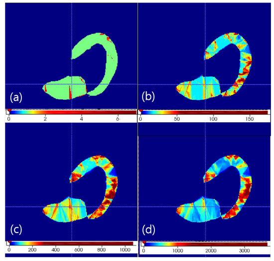
Figure 1.
Volume density of appearance texture with soft correspondence of m largest selection in any case. The axial view of the left heart is shown. (a) m = 1. (b) m = 2. (c) m = 3. (d) m = 4.
As this volume accumulation generated from this mapping uses much redundancy, we simplify volume accumulation into tetrahedron sets by using a filtering result of 3D Delaunay triangulation of M. This 3D Delaunay triangulation of the model points is performed with the alpha radius of 40 to remove noise tetrahedrons [31].
To extract one statistical model tetrahedron of all simplified , we use statistics in every . In the tetrahedron statistics calculation, tetrahedrons between the LV and LA also are considered as the cases of 0.5 probability in two objects. The tetrahedrons composed of only inner surface points of LV are not considered in the statistics. As common reference tetrahedrons are made from 3D Delaunay triangulation of M, statistics analysis is possible. As input of cascaded regression, atlas tetrahedron set is made by using tetrahedrons above threshold-probability of statistic probability accumulation array. Threshold-probability was selected as 14% under an empirical decision. Although the surface of the atlas tetrahedron set is not realistic, reconstructed makes realistic shapes in Figure 2. With the found , we make the final segmentation mask under the shape parameter set found.
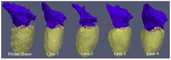
Figure 2.
Model tetrahedron set and, reconstructed of 4 cases. Five cases have the same tetrahedron cell topology and cell number.
2.5. Shape and Appearance Models
Because we can judge if (x, y, z) is inside , by simple calculation, the point set is constructed in a regular grid of 3D input. The group of a point set is concatenated with all tetrahedrons of , and it is denoted as . The array becomes a full set for the target points of appearance. From this array, a random selection of appearance is performed under a given number. The input image does not have any requirements in size and spacing, because appearance sampling is performed based on physical locations.
The transform between two images is constructed by piecewise-affine transform through the correspondence of tetrahedron vertexes. Specifically, the meshes of the training image have the same size because they are produced from the correspondence construction procedure. Between the atlas mesh and input mesh, we can perform a piecewise-affine transform [32]. Appearance correspondence can be constructed using these transforms. Because we know the point set of an atlas, we can rapidly extract the intensity and additional data of the training target by using the piecewise-affine transform on the point set.
The training input image is from a three-dimensional volume and two shapes are defined with and tetrahedron vertexes. The set of all vertexes is a vector that defines two models of the heart. This set is brought from a virtual correspondence point of group-wise correspondence construction procedure. Since the correspondence construction method makes similarity-free models, every shape correspondence does not have variations due to similarity transforms (translation, rotation, and scaling). PCA is applied to obtain the shape model. This shape model increases the number of eigenvectors independently with appearance information. The model is defined by the mean shape and the ith shape eigenvector of number. Shape eigenvectors are represented as columns of the matrix . This model also describes the ith eigenvalue . Finally, to model similarity transforms, is appended with six additional bases [33]. An instance of the shape model is constructed by
where is the vector of the shape parameters.
In order to learn the appearance model, each training image is warped to a reference frame by using to produce a similarity-free appearance. Since voxels in a tetrahedron are found by applying the piecewise-affine transform on the point set, an array of voxels included on each tetrahedron can be constructed rapidly. The total number of voxels on every tetrahedron is denoted as . Three features on one voxel are accumulated to construct an appearance set . The original intensity of the training image is used as the first feature, which is normalized with statistics in convex envelop volume of LV containing the cavity region of LV [33]. The sum of x, y, and z on the gradient is used as the second and third features, under Gaussian smoothing with 0.5 and 1.0. These three features are normalized by the z-score. Subsequently, only mean appearance is calculated.
2.6. Stochastic Cascaded Regression
Two points are manually selected as the initial location for the proposed method. The two points are the central locations of the LV and LA, and because they are selected on axial, sagittal, and coronal views by using ITKSNAP software [29], these central locations are relatively accurate initial locations. Moreover, while this initial location provides only scale and translation information, shape-deformation information must be determined using the segmentation program. The flow chart of the proposed method is shown in Figure 3.
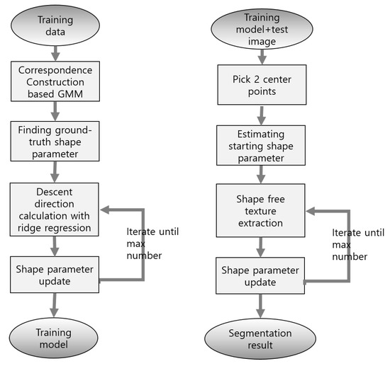
Figure 3.
Flow chart of SDM method. Training and test procedure are described.
Stochastic optimization was introduced by Robbin and Monro [34]. The approximation of the true gradient direction is realized by computing the gradient direction using only a small subset of randomly chosen samples in every iteration. In this manner, the computational cost per iteration is significantly reduced, while the convergence properties remain comparable to those obtained with deterministic gradient descent. The gradient direction is calculated in each iteration. Although the original cascaded regression method used all appearance sets owing to the small number of landmarks, the number of appearances can be too large in the proposed method because this framework is performed in 3D volume. To reduce computational cost and memory usage, we adopted a stochastic method by selecting a subset of the appearance set randomly. We denote the number of subsets in the appearance set as . This subset usage can substantially reduce the cost of ridge regression.
The ground-truth shape parameters are defined in each training image . After the ground-truth shape parameters are calculated in each training image, a set of perturbed shape parameters are generated for where t is the iteration number. This perturbation must capture the statistics of the heart-segmentation initialization process. SDM model of cascaded regression was used for the segmentation [11].
Generalized ridge regression (GRR) can be applied if the number of predictors p exceeds the sample size n [35]. Furthermore, GRR can apply different sparsity parameters to different groups of predictor variables. The present study used GRR as the ridge regression method because this method can implement additional selectiveness in the proposed framework. The work of removing features can be performed by increasing the sparsity parameter in the GRR framework. The procedure of GRR is explained conceptually in the following. After input data of the design matrix are rescaled by using the inverse square root of sparsity parameters, ridge regression is performed in the sparsity parameter of 1. The result vector is applied with rescaling again by using the inverse square root of the same scale sparsity parameters.
2.7. Evaluation Method
The training procedure is evaluated by the average error of the sample number in iteration t which is defined as follows:
The flow of this error is calculated in the training procedure to find an optimal sparsity parameter of ridge regression.
SSD is calculated by averaging the closest Euclidean distance using both directions between two surfaces. Three SSDs of the LV, LA, and left heart (LH) objects were evaluated. Hausdorff distance (HD) of the LV and LA, and Dice coefficient (DC) of LH were evaluated [36]. To compare our method to other methods, Microsoft Excel 2016 was used to generate descriptive statistics and perform paired t-tests. The significance levels were set to 0.05, 0.01, and 0.001.
3. Results
The proposed method was realized by C++ and ran on a Laptop with Intel Core i7-8750H, 16 GB RAM configuration. The perturbation number was 60 in the training image of 30 (or 29) in six groups. The grid spacing in appearance sampling was mm which caused the size of the point set () to be approximately 500,000. Since the appearance point numbers of the LA and LV were 500 and 500, the total appearance feature number () was 3000. The sparsity parameter of ridge regression was selected as 7500 empirically by considering the training profile of Equation (3). The shape eigen number () was selected as 26. This value includes six eigenvectors with similarity. Training of cascade regression needed 3496 ± 191 s in 10 iterations. Segmentation work needed 14.85 ± 7.31 s in 10 iterations.
3.1. System Evaluation
The evaluation metrics between two gold-standard masks of two operators were calculated for the comparison of difference. (1.06 ± 0.14 mm, 0.97 ± 0.12 mm, 1.02 ± 0.12 mm, 9.98 ± 2.83 mm, 10.60 ± 11.21 mm, 89.33% ± 1.87%) were the results of the evaluation, which are denoted as (LV SSD, LA SSD, LH SSD, LV HD, LA HD, LH DC). Since the extent of the structure in four major pulmonary vessels of LA might be different between two gold-standard masks, DC could be lowered to some degree. The repeatability of gold-standard generation can be estimated as 0.51 mm since the repeatability is calculated as the standard deviation of test sets.
According to Table 1, the proposed method produced a significantly better result in LH SSD and DC metric than every three methods. The group-wise method showed the performance improvement of LA SSD compared with the pairwise method from 2.88 ± 0.70 mm to 2.31 ± 0.53 mm. When the atlas of the LA was constructed in the pairwise correspondence method, the structure of four major pulmonary vessels was smoothed. This problem was removed in the proposed method. Group-wise method performs correspondence construction without separate object control. In LV, the inner and outer surface can have a dependence on the soft correspondence construction of GMM. The proposed method showed significantly better LV SSD of 1.94 ± 0.34 mm than 2.34 ± 0.44 mm of Group-wise method. Because of dependence in two surfaces of LV, Group-wise method’s LV SSD is worse than the pairwise method’s. In six-folds, training curves of the proposed method are shown in Figure 4.

Table 1.
Segmentation result comparison according to correspondence construction methods. This result is calculated with 35 cases under six-fold cross-validation.
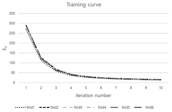
Figure 4.
Training curves of the proposed method in six-folds.
The iterative closest point (ICP) method minimizes the difference between two clouds of point [37]. We performed the ICP method with a trained shape model under six-fold cross-validation. Since point cloud extracted from gold-standard mask directly is used for registration of shape model, the appearance of LH is not considered in this registration. In Table 2, PairICP produced the significantly worse result in every metric than the cascaded segmentation of the pairwise method. However, GroupICP showed a registration result reaching the proposed method with a slight difference significance. If the ICP method is improved from simple ICP, then the registration result will be improved. DC was calculated under the appearance correspondence of cascaded regression.
Table 2.
ICP registration result comparison according to correspondence construction methods. This result is calculated with 35 cases under six-fold cross-validation.
We tested the proposed method by varying the vertex number of 3D model in Table 3. Experiments only show that a small of 3000 or 4500 can degrade the segmentation accuracy. As statistics is 9219 ± 1696, a selection of 3000 and 4500 can make shape loss. Since there is not much difference between 6000 and 7500, we selected 6000 as in experiments of Table 1 and Table 2.
Table 3.
Segmentation results of group-wise separate according to vertex number of 3D model . This result is calculated with 35 cases under six-fold cross-validation.
As the additional experiment, we checked which model is better between a combined model of two objects and a separate shape model. We can duplicate the shape eigenvector and set the other part of this eigenvector to zero. Under this condition, a combined model with 26 shape eigenvectors extended to a separate model with 46 eigenvectors. The number 6 here is the number of shape eigenvectors. The evaluation result of the separate model in of 6000 was (1.91 ± 0.37 mm, 2.24 ± 0.52 mm *, 2.07 ± 0.32 mm **, 14.38 ± 2.82 mm, 19.21 ± 5.18 mm, 81.45% ± 3.84%***), where * 0.05, ** 0.01, and *** 0.001. All p values derive from paired t-tests comparing the separate model with the proposed method. The separate model with 46 eigenvectors was slightly better than the proposed method, although conflict between LA and LV could occur in a separate model.
3.2. Comparison with Other Methods
Tran et al.’s method uses a deep, fully convolutional neural network for ventricle segmentation in cardiac MRI [18]. This method evaluates the surface distance of 30 cases on the LV’s endocardial and epicardium surfaces. The endocardial surface error was 1.73 ± 0.35 mm, and the epicardium surface error was 1.65 ± 0.31 mm. Tran et al.’s method was evaluated only on the ventricle model. Although the repeatability is not considered in the evaluation metric calculation, the proposed method shows a comparable accuracy of 1.88 ± 0.37 mm. Mitchell et al.’s method uses a 3D active appearance model and produced an error of 2.75 ± 0.86 mm for endocardial contours and 2.63 ± 0.76 mm for epicardium contours, which were evaluated on 359 slices of cardiac MRI [6]. Compared with this result, our method shows a better accuracy of 1.88 ± 0.37 mm in LV SSD. Tölli et al.’s method performed the segmentation of four-chamber model by using artificially enlarged training set and Active Shape Model-based segmentation in 25 subjects. This method produced 1.77 ± 0.36 mm in LV, and 2.44 ± 0.85 mm in LA, although the enlargement method of training set is used [38]. Our method shows a better result in LA, compared with this method. Zhuang et al. evaluated whole heart segmentation under deep learning (DL) based-method and multi atlas segmentation (MAS) frameworks [36]. This evaluation result shows mean SSD of 2.12 ± 5.13 mm and mean DC of 87.20% ± 8.70%. Range of DC can be different from that of the proposed method because the characteristics of the two datasets are different. In this Open-Access Grand Challenge, the active appearance-based method is not utilized. If the current research includes whole heart components, we can also apply to a challenge like this.
3.3. Examples of the Segmentation Result
Three examples of the proposed method with of 7500 are presented in Figure 5, Figure 6 and Figure 7. Figure 5 presented the best case. Figure 6 presented the median case. The boundary of LV is not captured exactly. Figure 7 presented the worst case. The statistics of LV is not learned properly since training images do not contain such images enough.
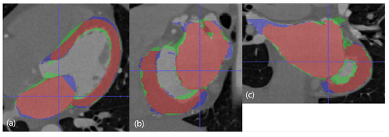
Figure 5.
The best case in the dimension of DC. The red resultant mask is true positive, the blue mask is false negative, and the green resultant mask is false positive. SSD, HD, and DC are presented as the (LV SSD, LA SSD, LH SSD, LV HD, LA HD, DC) set, which is (1.79 mm, 1.74 mm, 1.77 mm, 17.74 mm, 17.78 mm, 85.95%). (a) Axial view. (b) Sagittal view. (c) Coronal view.
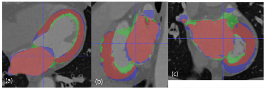
Figure 6.
The median case in the dimension of DC. The red resultant mask is true positive, the blue mask is false negative, and the green resultant mask is false positive. SSD, HD, and DC are presented as the (LV SSD, LA SSD, LH SSD, LV HD, LA HD, DC) set, which is (1.79 mm, 2.16 mm, 1.98 mm, 11.29 mm, 19.91 mm, 81.88%). (a) Axial view. (b) Sagittal view. (c) Coronal view.
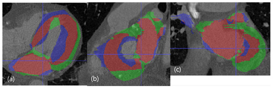
Figure 7.
The worst case in the dimension of DC. The red resultant mask is true positive, the blue mask is false negative, and the green resultant mask is false positive. SSD, HD, and DC are presented as the (LV SSD, LA SSD, LH SSD, LV HD, LA HD, DC) set, which is (2.79 mm, 2.09 mm, 2.44 mm, 16.80 mm, 17.43 mm, 67.58%). (a) Axial view. (b) Sagittal view. (c) Coronal view.
4. Discussion
Multi-objects modeling in cascaded regression is under development. In the correspondence construction of the GMM-based method, the dependence of multi-objects must be considered, although training procedure is performed in combined shape. If the vertex number of 3D model is increased to cover many objects, computation resources will increase rapidly. There is a trade-off between memory problems and shape loss in separate and combined constructions of correspondences.
Segmentation accuracy depends on the quality of tetrahedron set since the final segmentation region is calculated by checking inside of the tetrahedron set. In the proposed method, several heuristics rules are adapted to tetrahedron statistics calculations. A more systemic rule must be developed to increase the quality of segmentation shape from the found point set.
Separate operation of correspondence construction is made from the input sort array of training points. Since statistics of sorts is calculated accurately by using , we apply this sort of information to statistical analysis of tetrahedron . Tetrahedron between LA and LV can have noises since the topology between LA and LV is complex. More fine control is needed, especially in the region between LA and LV.
The separate shape model of duplicate eigenvectors gave more freedom in shape change and produced a slightly better evaluation result than the proposed method. But since the conflict between LA and LV could occur, a check of conflict must be performed to use this model. Since this conflict check between objects needs an additional computation, the combined shape model can be used instead.
Since unit-vector normalization makes the contents of appearance too small, z-score normalization is applied to the appearance input of ridge regression. Furthermore, ridge regression is not scale-invariant. If the scales used to express the individual appearance variables are changed, then the ridge coefficients do not alter in inverse proportion to the changes in the variable scales [39]. Therefore, z-score normalization is assumed to produce better scaling in terms of data size.
In the future, the segmentation model for dealing with every phases of the heart must be developed, since the statistics of the systole phase make DC be comparatively low value. If an extensive database is applied, memory problems and many technical problems will occur since cascaded regression needs texture modeling compared with an active shape model. To improve the segmentation result, then many cases must be applied to construct the heart anatomical model. Finally, readjustment of segmentation surfaces by using boundary normal direction can be developed to increase the segmentation performance by including this post-processing in active appearance framework.
5. Conclusions
We developed a cascaded regression framework for 3D cardiac CT segmentation. In the GMM-based correspondence construction method, the appearance correspondence extraction method is proposed to extend this correspondence method to model-based segmentation. An independant final point correspondence construction method is developed to apply the GMM-based correspondence method to the double-shaped model of LH. Stochastic appearance selection enables effective construction in the aspect of memory usage and computation time. A comparison between the two state-of-art correspondence construction methods was performed in segmentation accuracy. By using a constructed cardiac model, the rapid segmentation of three-dimensional anatomical models could support diagnosis and help navigate mapping and ablation catheters off complex structures such as the LA.
Author Contributions
Conceptualization, J.P.B. and D.L.; Methodology, J.P.B., M.V. and S.Y.; Software, J.P.B. and S.C.; Data curation, S.Y. and C.H.Y.; Writing–original draft preparation, J.P.B.; Project administration, D.L.; Writing—review and editing M.V. and D.L. All authors have read and agreed to the published version of the manuscript.
Funding
This work was supported by KIST intramural grants (2E30260).
Conflicts of Interest
There is no conflict of interest related to this work.
Abbreviations
| Set of similarity transforms | |
| Similarity transform of k training data | |
| Model tetrahedron set under set | |
| Each tetrahedron set under set | |
| Set of training point sets | |
| Three dimensional training point set of k training data | |
| Spatial coordinates of each point | |
| Model point set | |
| Model point | |
| Posterior probability indexed k, i and j | |
| Subset of input point set under object b | |
| Virtual correspondence point | |
| Temporary virtual correspondence point under object b | |
| flag matrix for object label | |
| Integer | |
| Result tetrahedron set of constrained triangulation constructed under | |
| i point of one tetrahedron l | |
| Appearance point set | |
| Concatenated full appearance set | |
| b | Index of three objects which are left atrium, inner surface and outer |
| surface of left ventricle | |
| Training volume image | |
| , | Two tetrahedron vertex numbers of double shapes |
| Mean shape | |
| ith shape eigenvector | |
| Shape eigenvectors | |
| Eigenvalue of | |
| Vector of shape parameters | |
| Mean appearance | |
| Ground-truth shape parameters | |
| Perturbed shape parameters of iteration t | |
| Number of shape perturbation | |
| Voxel number of selected appearance subset | |
| Total number of voxels on every tetrahedron | |
| Number of shape eigenvectors | |
| Number of training set | |
| Vertex number of k training point set | |
| Vertex number of 3D model | |
| Number of tetrahedrons on model tetrahedron set | |
| Total tetrahedron number under |
References
- Schoenhagen, P.; Stillman, A.E.; Halliburton, S.S.; White, R.D. CT of the heart: Principles, advances, clinical uses. Clevel. Clin. J. Med. 2005, 72, 127–138. [Google Scholar] [CrossRef] [PubMed]
- Haissaguerre, M.; Jais, P.; Shah, D.C.; Takahashi, A.; Hocini, M.; Quiniou, G.; Garrigue, S.; Le Mouroux, A.; Le Métayer, P.; Clémenty, J. Spontaneous initiation of atrial fibrillation by ectopic beats originating in the pulmonary veins. N. Engl. J. Med. 1998, 339, 659–666. [Google Scholar] [CrossRef] [PubMed]
- Sra, J.; Krum, D.; Malloy, A.; Vass, M.; Belanger, B.; Soubelet, E.; Vaillant, R.; Akhtar, M. Registration of three-dimensional left atrial computed tomographic images with projection images obtained using fluoroscopy. Circulation 2005, 112, 3763–3768. [Google Scholar] [CrossRef] [PubMed]
- Sra, J.; Krum, D.; Hare, J.; Okerlund, D.; Thompson, H.; Vass, M.; Schweitzer, J.; Olson, E.; Foley, W.D.; Akhtar, M. Feasibility and validation of registration of three-dimensional left atrial models derived from computed tomography with a noncontact cardiac mapping system. Hear. Rhythm. 2005, 2, 55–63. [Google Scholar] [CrossRef]
- Vania, M.; Mureja, D.; Lee, D. Automatic spine segmentation from CT images using convolutional neural network via redundant generation of class labels. J. Comput. Des. Eng. 2019, 6, 224–232. [Google Scholar] [CrossRef]
- Mitchell, S.C.; Bosch, J.G.; Lelieveldt, B.P.F.; der Geest, R.J.; Reiber, J.H.C.; Sonka, M. 3-D active appearance models: Segmentation of cardiac MR and ultrasound images. IEEE Trans. Med. Imaging 2002, 21, 1167–1178. [Google Scholar] [CrossRef] [PubMed]
- Zheng, Y.; Barbu, A.; Georgescu, B.; Scheuering, M.; Comaniciu, D. Four-chamber heart modeling and automatic segmentation for 3-D cardiac CT volumes using marginal space learning and steerable features. IEEE Trans. Med. Imaging 2008, 27, 1668–1681. [Google Scholar] [CrossRef]
- Depa, M.; Sabuncu, M.R.; Holmvang, G.; Nezafat, R.; Schmidt, E.J.; Golland, P. Robust atlas-based segmentation of highly variable anatomy: Left atrium segmentation. In International Workshop on Statistical Atlases and Computational Models of the Heart; Springer: Berlin/Heidelberg, Germany, 2010; pp. 85–94. [Google Scholar]
- Cheng, R.; Roth, H.R.; Lu, L.; Wang, S.; Turkbey, B.; Gandler, W.; McCreedy, E.S.; Agarwal, H.K.; Choyke, P.; Summers, R.M.; et al. Active appearance model and deep learning for more accurate prostate segmentation on MRI. In SPIE Medical Imaging 2016: Image Processing; International Society for Optics and Photonics: San Diego, CA, USA, 2016; p. 97842I. [Google Scholar]
- Cootes, T.F.; Edwards, G.J.; Taylor, C.J. Active appearance models. IEEE Trans. Pattern Anal. Mach. Intell. 2001, 23, 681–685. [Google Scholar] [CrossRef]
- Xiong, X.; la Torre, F. Supervised descent method and its applications to face alignment. In Proceedings of the IEEE Conference on Computer Vision and Pattern Recognition, Portland, OR, USA, 23–28 June 2013; pp. 532–539. [Google Scholar]
- Dollár, P.; Welinder, P.; Perona, P. Cascaded pose regression. In Proceedings of the 2010 IEEE Computer Society Conference on Computer Vision and Pattern Recognition, San Francisco, CA, USA, 13–18 June 2010; pp. 1078–1085. [Google Scholar]
- Tzimiropoulos, G. Project-out Cascaded Regression with an Application to Face Alignment. In Proceedings of the IEEE Conference on Computer Vision and Pattern Recognition, Boston, MA, USA, 7–12 June 2015; pp. 3659–3667. [Google Scholar]
- Asthana, A.; Zafeiriou, S.; Cheng, S.; Pantic, M. Incremental face alignment in the wild. In Proceedings of the IEEE Conference on Computer Vision and Pattern Recognition, Columbus, OH, USA, 23–28 June 2014; pp. 1859–1866. [Google Scholar]
- Ren, S.; Cao, X.; Wei, Y.; Sun, J. Face alignment at 3000 fps via regressing local binary features. In Proceedings of the IEEE Conference on Computer Vision and Pattern Recognition, Columbus, OH, USA, 23–28 June 2014; pp. 1685–1692. [Google Scholar]
- Ecabert, O.; Peters, J.; Schramm, H.; Lorenz, C.; Berg, J.V.; Walker, M.J.; Vembar, M.; Olszewski, M.E.; Subramanyan, K.; Lavi, G.; et al. Automatic Model-Based Segmentation of the Heart in CT Images. IEEE Trans. Med. Imaging 2008, 27, 1189–1201. [Google Scholar] [CrossRef]
- Zheng, Y.; Yang, D.; John, M.; Comaniciu, D. Multi-part modeling and segmentation of left atrium in C-arm CT for image-guided ablation of atrial fibrillation. IEEE Trans. Med. Imaging 2013, 33, 318–331. [Google Scholar] [CrossRef] [PubMed]
- Tran, P.V. A fully convolutional neural network for cardiac segmentation in short-axis MRI. ArXiv 2016, arXiv:1604.00494. [Google Scholar]
- Payer, C.; Štern, D.; Bischof, H.; Urschler, M. Regressing heatmaps for multiple landmark localization using CNNs. In International Conference on Medical Image Computing and Computer-Assisted Intervention; Springer: Berlin/Heidelberg, Germany, 2016; pp. 230–238. [Google Scholar]
- Payer, C.; Štern, D.; Bischof, H.; Urschler, M. Multi-label whole heart segmentation using CNNs and anatomical label configurations. In International Workshop on Statistical Atlases and Computational Models of the Heart; Springer: Berlin/Heidelberg, Germany, 2017; pp. 190–198. [Google Scholar]
- de Vos, B.D.; Wolterink, J.M.; de Jong, P.A.; Leiner, T.; Viergever, M.A.; Išgum, I. ConvNet-based localization of anatomical structures in 3-D medical images. IEEE Trans. Med. Imaging 2017, 36, 1470–1481. [Google Scholar] [CrossRef]
- Wang, C.; Smedby, Ö. Automatic multi-organ segmentation in non-enhanced CT datasets using hierarchical shape priors. In Proceedings of the 2014 22nd International Conference on Pattern Recognition, Stockholm, Sweden, 24–28 August 2014; IEEE: Piscataway, NJ, USA, 2014; pp. 3327–3332. [Google Scholar]
- Wang, C.; Smedby, Ö. Automatic whole heart segmentation using deep learning and shape context. In International Workshop on Statistical Atlases and Computational Models of the Heart; Springer: Berlin/Heidelberg, Germany, 2017; pp. 242–249. [Google Scholar]
- Granger, S.; Pennec, X. Multi-scale em-icp: A fast and robust approach for surface registration. In European Conference on Computer Vision; Springer: Berlin/Heidelberg, Germany, 2002; pp. 418–432. [Google Scholar]
- Hufnagel, H.; Pennec, X.; Ehrhardt, J.; Ayache, N.; Handels, H. Generation of a statistical shape model with probabilistic point correspondences and the expectation maximization-iterative cloest point algorithm. Int. J. Comput. Assist. Radiol. Surg. 2008, 2, 265–273. [Google Scholar] [CrossRef]
- Gooya, A.; Davatzikos, C.; Frangi, A.F. A bayesian approach to sparse model selection in statistical shape models. SIAM J. Imaging Sci. 2015, 8, 858–887. [Google Scholar] [CrossRef]
- Chui, H.; Rangarajan, A.; Zhang, J.; Leonard, C.M. Unsupervised learning of an atlas from unlabeled point-sets. IEEE Trans. Pattern Anal. Mach. Intell. 2004, 26, 160–172. [Google Scholar] [CrossRef]
- Frangi, A.F.; Rueckert, D.; Schnabel, J.A.; Niessen, W.J. Automatic construction of multiple-object three-dimensional statistical shape models: Application to cardiac modeling. IEEE Trans. Med. Imaging 2002, 21, 1151–1166. [Google Scholar] [CrossRef]
- Yushkevich, P.A.; Piven, J.; Hazlett, H.C.; Smith, R.G.; Ho, S.; Gee, J.C.; Gerig, G. User-guided 3D active contour segmentation of anatomical structures: Significantly improved efficiency and reliability. Neuroimage 2006, 31, 1116–1128. [Google Scholar] [CrossRef]
- Lorensen, W.E.; Cline, H.E. Marching cubes: A high resolution 3D surface construction algorithm. ACM Siggraph Comput. Graph. 1987, 21, 163–169. [Google Scholar] [CrossRef]
- Edelsbrunner, H. Alpha shapes—A survey. Tessellations Sci. 2010, 27, 1–25. [Google Scholar]
- Matthews, I.; Baker, S. Active appearance models revisited. Int. J. Comput. Vis. 2004, 60, 135–164. [Google Scholar] [CrossRef]
- Andreopoulos, A.; Tsotsos, J.K. Efficient and generalizable statistical models of shape and appearance for analysis of cardiac MRI. Med. Image Anal. 2008, 12, 335–357. [Google Scholar] [CrossRef] [PubMed]
- Robbins, H.; Monro, S. A stochastic approximation method. Ann. Math. Stat. 1951, 400–407. [Google Scholar] [CrossRef]
- Ishwaran, H.; Rao, J.S. Geometry and properties of generalized ridge regression in high dimensions. Contemp. Math. 2014, 622, 81–93. [Google Scholar]
- Zhuang, X.; Li, L.; Payer, C.; Štern, D.; Urschler, M.; Heinrich, M.P.; Oster, J.; Wang, C.; Smedby, Ö.; Bian, C.; et al. Evaluation of algorithms for Multi-Modality Whole Heart Segmentation: An open-access grand challenge. Med. Image Anal. 2019, 58, 101537. [Google Scholar] [CrossRef]
- Besl, P.J.; McKay, N.D. Method for registration of 3-D shapes. In Sensor Fusion IV: Control Paradigms and Data Structures; International Society for Optics and Photonics: Boston, MA, USA, 1992 Volume 1611; pp. 586–606. [Google Scholar]
- Tölli, T.; Koikkalainen, J.; Lauerma, K.; Lötjönen, J. Artificially enlarged training set in image segmentation. In International Conference on Medical Image Computing and Computer-Assisted Intervention; Springer: Berlin/Heidelberg, Germany, 2006; pp. 75–82. [Google Scholar]
- Breiman, L. Better subset regression using the nonnegative garrote. Technometrics 1995, 37, 373–384. [Google Scholar] [CrossRef]


© 2020 by the authors. Licensee MDPI, Basel, Switzerland. This article is an open access article distributed under the terms and conditions of the Creative Commons Attribution (CC BY) license (http://creativecommons.org/licenses/by/4.0/).