Abstract
A balance control method, the proportional-integral sliding mode control (PISMC), is proposed to control the tilt attitude of an experimental two-wheel vehicle system (TWVS). Based on our previous work of implementing a generalized PISMC to control a linearized dynamical system, this paper extends the algorithm to a wider range: First, the control design of a weighted-control system is proposed. Secondly, our algorithm was realized and verified in a TWVS using its original nonlinear model. Thirdly, a systematical way to tune parameters are presented. The robustness of the proposed algorithm is also discussed in this paper. The simulation results of this work validate that the PISMC has better robustness to counteract the external disturbances than the conventional sliding mode control (SMC) does. Additionally, the experimental results show that the PISMC is capable of autonomously balancing the TWVS more effectively than the conventional SMC. The successful implementation of our algorithm potentially extends the implementation of the PISMC to various nonlinear and emerging systems.
1. Introduction
This paper presents a controller called the proportional-integral sliding mode controller (PISMC). The sliding mode control (SMC) has been widely accepted as an efficient method for the tracking or balance control of an uncertain nonlinear system. The capability of achieving perfect performance in principle is also demonstrated in the presence of parameter uncertainties and bounded external input disturbances. The proposed PISMC combines the proportional sliding mode control (PSMC) and the integral sliding mode control (ISMC). There are two main contributions in this paper. First, the PISMC provides more parameters with which to tune the controller. As a consequence, it reduces adverse effects due to the external disturbances effectively. Second, this paper sets up an experiment as an example to demonstrate the tracking accuracy in a nonlinear system. This example also shows how this algorithm can be implemented to a physical system. Though the name PISMC may sound similar to some algorithms regarding the PID sliding surface, the definition of sliding surface and the mathematical expression of PISMC are different.
The main structure of SMC theory was brought out by Utkin, a former USSR scholar, in 1977 [1]. After the original theory, various applications and extensions of the theory were proposed and presented. Some of the examples are given and reviewed in the following. In 1994, Sira-Ramirez et al. [2] proposed a dynamic multivariable discontinuous feedback control strategy of the sliding mode type for the altitude stabilization of a nonlinear helicopter model in vertical flight. In 1996, Utkin and Jingxin [3] proposed a new sliding mode design concept named integral sliding mode control (ISMC). ISMC is different from the conventional sliding mode design approaches, and the only difference is the integral form of the error term in place of the original error term. In 2000, Baik et al. [4] designed an ISMC which has one separate boundary surface in order to decrease the chattering and improve the controllers’ responses. In 2003, Lin et. al [5] proposed a PID sliding surface, where the sliding mode motion occurs with global invariance. In the same year, Hess and Wells [6] employed the SMC for flight control design. In 2004, Rafimanzelat and Yazdanpanah [7] investigated the low chattering SMC for balance control design. In 2005, Niu and Ho et al. [8] applied the robust integral sliding mode control to uncertain stochastic systems. Besides that, Waslander et al. applied the design of ISMC to a multi-agent quadrotor test-bed. Moreover, Bouabdallah, et al. also applied the back-stepping and sliding-mode techniques to an indoor micro-quad-rotor. Koshkouei et al. [9] in 2005 proposed a dynamic SMC which increases accuracy under high-frequency switching of control. More studies regarding the applications of sliding mode technique and its extensions are discussed in [10,11,12,13]. In 2009, Soylu et al. [14] studied the control of an underwater remote vehicle-manipulator system using sliding-mode control and control. This paper showed that the sliding-mode and controller combined approach provides superior dynamic coupling reduction performance.
Speaking of PISMC, Nawawi, Sam, and Osman have devoted themselves to the investigation of PISMC [15,16,17,18] since 2002. In 2011, Lin et al. applied the PISMC to stabilize the attitude and position of a hovering unmanned helicopter [19]. Sam at al. applied the PISMC to a hydraulically-actuated active suspension system [17,18]; Nawawi, et al. focused on the control and manipulation of of robotic systems. [15,16]. In [20], robust integral sliding mode control (ISMC) was proposed for an underactuated rotary hook system in order to deal with parametric uncertainties presenting themselves in the system’s parameters. Pan et al. studied the modification of the integral sliding variable degrades, and suggested that the switching element is smoothed by using a low-pass filter [21]. More works related to sliding mode control can be found in [22,23]. In [22] a SMC was designed to control a washout filter with constant impedance and nonlinear constant power loads. In [23] a PDSMC was designed to collaborate with a sliding perturbation observer to control a robot manipulator.
One thing to note is the work, cited in [15], done by Nawai et al. in 2006. In this reference, Nawawi suggested PISMC for the two-wheel inverted pendulum mobile robot to avoid high chattering drawbacks. Even though [15] had a similar topic and methodology to this paper, the details were significantly different. In [15], a linear model was investigated; the proportional and integral sliding modes shared the same coefficient, and the integration applied to the derivative of the states. In this paper, nevertheless, there are three major differences. First, we do not restrict our system to a linear one. Actually, the examples in this paper were presented and controlled using the original nonlinear form. Second, we introduce two parameters, instead of one coefficient as in [15], in the investigation. This setting provides us more degrees of freedom to tune parameters and improve the system performance. Third, in the integral we include not only the derivative of the states, but also the states themselves through the error term. Consequently, the work described here and our contributions in the PISMC apparently differ from those made by other researchers.
More specifically, we cite the following list the differences from [15]:
- Design of sliding surface for the controlled system: Our paper presents . In [15], the sliding surface was designed as .
- The system of control in this paper is nonlinear, whereas the system in [15] was a linearized system.
- Because the system to control in [15] was linear, their proposed controller was merely a function of the system, given bywhere f is the original form representing a nonlinear function describing the deviation from linearity in term of disturbances and un-modeled dynamics. Our controller, however, has two major differences from theirs: First, we do not employ the remainder of the nonlinearity terms directly. Instead, we employ the bound of the remainder nonlinearity terms. Secondly, the saturation function in our controller is more than a sgn function; the selection of parameters is different.
- The tuning procedures of parameters are discussed in this paper, but not in [15].
The work presented in this paper extends the work presented in [19] to a wider range. The following novelties or contributions are presented in this paper. First, differently from the commonly known ISMC, PISMC, and PID sliding surface, which usually each have the sliding surface of and five parameters or more to tune, our algorithm in [19] extends the sliding surface to the nth order derivative of the output error with only two parameters to tune. In [19], however, a system of unweighted control was considered. Based on the work in [19], this paper proposes the sufficient condition to design a control for a system of weighted control. Secondly, our algorithm was realized and verified in a two wheel vehicle system. In the literature, researchers either applied their work to nonlinear systems using numerically simulated results [21,24], or realized their algorithms in a linear system [20,22,23]. Although nonlinearities were considered in [22,23], they were treated as disturbances instead of dynamics themselves. This paper not only verifies our capability of controlling a nonlinear system by numerical simulations, but also realizes the algorithms in a TWVS using its original nonlinear model. Instead of treating the nonlinearities as disturbances like works in the literature, we dealt with the nonlinearity as the dynamics itself. The successful implementation of our algorithm in a practical nonlinear mechanical system indicates that it is possible to extend the application of the PISMC to a wide range of nonlinear systems, such as the control of microfluidics-based devices [25,26]. Thirdly, tuning of control parameters is always critical in designing a control. In our proposed algorithms, there are only four parameters to tune for all systems. From analysis and past experience, we roughly understand the effects of these parameters, though they were not rigorously proven. Systematic tuning procedures are also presented in this paper.
In detail, we first briefly review the SMC and PSMC and their drawbacks. The algorithms and control law by PISMC are then introduced. Before applying the PISMC control law to real cases, robustness, systematic tuning procedures, and performance are then discussed. Having shown the robustness and good performance of our algorithm, the control design for a weighted-control system is proposed. This paper then derives the dynamic model of an experimental TWVS with given parameters. The PISMC was designed based on the TWVS model, and all the input information was obtained from the real tests which were conducted by the TWVS. The corresponding control to stabilize the TWVS was derived based on the proposed PISMC algorithm, and tested in experiments. Discussion of experimental results and a conclusion are provided to demonstrate the validity of our proposed algorithm.
2. Control Algorithm
2.1. Conventional Sliding Mode Control
The theory of SMC has been extensively applied in linear and nonlinear systems, and different practical engineering control problems. Studies in the past few decades have demonstrated that the SMC methodology provides a systematic approach to solving control engineering problems. By introducing a sliding mode to the control of a system, one can achieve both stabilization and disturbance rejection.
The conventional PSMC is considered as a proportional type which forces system states to slide into the predetermined sliding surface, and to reach the origin of the phase plane eventually. When the state-trajectory is sliding on the sliding surface, the corresponding dynamic performance of the system is governed by the equations of the sliding surface. Therefore, the PSMC has a strong robustness against external uncertainties and disturbances.
There are two major requirements for the PSMC. The first one is to design a sliding surface. Then the states are enforced to slide into the sliding surface by the switching the control law. Secondly, each of the tracking points on the sliding surface must satisfy the sliding conditions. The switch of the control law is determined by the predefined switching conditions. With the help of the control switch, the trajectory can be guided into the region bounded by boundary layers. Governed by the sliding conditions, the trajectory gradually moves onto the sliding surface and steps forward to the target point.
Consider a desired signal and the system output , where both of and are in . The objective of the PSMC is to make the system’s output approach the desired signal when ; i.e.,
Here, we define the tracking error as
where . Before the PSMC is applied, a sliding surface must be designed in advance. The goal of the PSMC is to guide the system trajectory toward the sliding surface, which naturally leads the trajectory to the target point in the end. Based on the magnitude of errors, we define a time-varying linear differential function in , , named the condition space [27], given by
where is a positive constant. The equation represents a sliding surface passing through the origin of the phase plane. According to the above equation, is an th-order linear differential equation, and all the eigenvalues of the characteristic equation are located in the left complex plane. Once the sliding surfaces are determined, we may start to design the controller and define the sliding conditions as follows [27].
where , and denotes the time derivative of s.
2.2. Proportional-Integral Sliding Mode Control
To improve the performance of a SMC, this paper adopts a PISMC as our algorithm. Consider a dynamic system described by an nth-order nonlinear differential equation
where is the output of the dynamic system, f is the system function and must be at least once differentiable, is the system input, and t is time. We define the state vector, , for future derivations.
Assumption 1.
Consider (6) and assume that there exists an uncertain parameter in the dynamic function , satisfying
where is the estimation and is the variation of function f. Assume
given the boundary of system uncertainty [27].
The goal of the PISMC proposed in this paper is to design a switching control law to let the output approach a given , as shown in (2). To design the control system, the system states are assumed to be attainable via a state observer, which sometimes requires measurement of an output or output error, as defined in (3). The sliding surface of the PISMC consists of two sliding surfaces, and , the proportional sliding surface and the integral sliding surface, respectively. Here,
as defined in (4), and
where , , . The operator is defined as
where is a parameter to tune, and denotes the k-combinations of a set having n elements. Applying the operator to a function yields
where the superscript with parentheses denotes the order of derivative, while the superscript without parentheses denotes the power of the parameter . In our case, or . They are two complementary parameters, which provide the capability of tuning the gains of controller. We note that the expansion of (9) is different from the conventional PSMC or PID sliding surface, since and are generally distinct. The PISMC is designed as [19]:
where, by letting ,
with
and
The controller design is summarized in Theorem 1.
Theorem 1.
[19] Consider the system of (6) which satisfies Assumption 1. Let the function be specified in (12) with being equivalent signal and being switching control defined in (13) and (14), respectively. The gain k is designed to satisfy (5) with the definition of given in (15). If there is a k and an such that
then the tracking error as defined in (3) will tend to a neighborhood of zero within a finite time.
Proof.
The proof is a brief version of [19] for further usage. Define the following Lyapunov function
Choose an appropriate to satisfy . Then,
The sufficient condition of (18) to ensure the stability of system and to satisfy the sliding conditions as in (5) is given by
Let
provided . We conclude
as stated in (16). It is also conclusive from (18) that converges to the neighborhood around origin of the phase plane for any trajectory. □
In fact, in the control signal there is a the discontinuous contribution , caused by the discontinuous switching function (). This function results in an infinitely large switching frequency. However, this infinitely large switching frequency can not be realized in real physical system. Therefore, a switching component with extremely high-speed is applied. That way, the state trajectory would oscillate around the two sides of which results in the chattering phenomenon.
In order to reduce the chattering problem, the concept of boundary layers for a sliding surface is employed, as depicted in Figure 1.
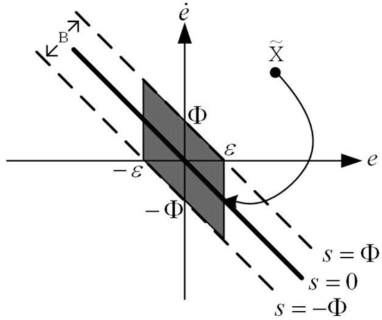
Figure 1.
The definition of boundary layer for a sliding surface [19].
The definition of boundary layers is given by
The error phase-plane of boundary layers of a sliding surface, s, coincides with the boundary range of . Note that is the boundary layer. Since the switch action can not be completed in a blink of time and the effect of delay exists, the state trajectory would oscillate between the boundary layers. Figure 1 is the 2nd-order error phase plane, and it is the most common way to mitigate the oscillation by replacing the sliding surface with the boundary layers. is the switching law of the controller, defined as follows
Here sat is the saturation function defined by
2.3. Alternative from of the Controller
In this paper, we assume that all states are attainable via state observers, but do not touch the design of the observer. The original design of the controller in (12) may require additional estimation of , which may need to employ new gain(s).
In order to avoid this drawback, an alternative design of is proposed by reducing the order of . (3) leads to
To have , the control was originally designed as
where , and
As a result, (22) can be rewritten as
or,
To eliminate , we here re-design as
That is, replace the original by letting
We claim that this controller works, and this controller does not need to measure .
The proof is given as follows:
2.4. Robustness Discussion
Unlike the design concept of conventional SMC, the insensitivity is included in the dynamics model and also guaranteed in our algorithm. In the conventional SMC design, a precise dynamics model is employed and the perturbation is viewed as an extra input. An example is given in Equation (22) in [28]. The change rate of s is formulated by
and the robustness is discussed based on this formulation. In our approach, however, the perturbations are already included in the parameter k for . Recall that , where is the bound of the model variation, satisfying and
Let , where is the nominal states. Then,
where and includes all the remainder terms. By properly investigating and choosing the bound of . The influence of perturbations is included and considered in the control. The advantage of our approach is that the robustness of the control is guaranteed with a proper choice of , and we do not have to worry about specific perturbations. The drawback, of course, it that the control might be inefficient if is defined too large for the purpose of robustness.
2.5. Parameter Tuning
In the proposed algorithm, there are four parameters to tune in total: and to construct s-surface, to construct , and to determine the saturation function. We have tried to analytically understand the effect of each parameter. However, this is too difficult due to the complexity of nonlinear systems and mathematics. Instead, approximated properties in a 2nd order system are analyzed, and numerical simulations are presented to demonstrate the potential effect of each parameter, so that readers will have some ideas on our tuning procedures. Notably, numerical examples are not solid proofs. An effect may vary in different cases.
The example from [19] is employed to study the effect of each parameter, and how to tune these parameters. The example, given as follows, was originally from [27] and employed to demonstrate the validity of the our proposed algorithm:
The function is unknown but varies within the range . Let
The control input of SMC is
with . The control input of PISMC is
with
Notably, we employed this example in our work in [19], and showed the validity of our work. In this paper, however, we employ this example to show the properties and influences of parameters. As a result, despite the dynamical equation and parameters of the equation being directly employed from [27], other settings are changed. For example, we used state errors and their derivatives, instead of the output rate in the reference. The parameters of the controller are different from those in the reference. The desired signal is set as unit step for investigating transient properties, which is different from the original . Therefore, the comparison occurs between our PISMC and SMC to know the parameters better. It did not occur between our PISMC and the SMC of the reference.
2.5.1. Effect of
is the parameter to determine the switching method and reduce the chattering phenomenon, as shown in (21). However, the larger the value of , the more sluggish the response. As , sat() = . As , sat() = sgn(s), which usually causes chattering phenomenon. Consider the case , so that sat() = . Since s is finite in general, . The smaller the , the smaller the . The decreasing rate of the Lyapunov function is influenced by
The original saturation function sat() = sgn(s) brings . The condition to have a more greatly decreasing rate of the Lyapunov function is given by
or equivalently, . Therefore, a large is not helpful in speeding up the converge of the system. Figure 2 demonstrates the comparison. in Figure 2a, whereas in Figure 2b. Other parameters are set identical. It is obvious that the responses with smaller are faster, regardless of the type of controls.

Figure 2.
Comparison of parameter effectiveness. (a) ; (b) .
2.5.2. Effect of
It can be expected that the larger the value of , the more decreasing the rate of the Lyapunov function from . Suppose at beginning. The upper bound for is given in (33). Since , we conclude the upper bound of V satisfies
(35) implies that V converges exponentially with time constant .
Figure 3 demonstrates the comparison. in Figure 3a, whereas in Figure 3b. Other parameters are set identically. It is obvious that the responses with large are faster, regardless of the type of controls.
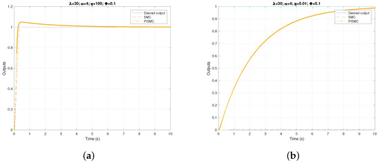
Figure 3.
Comparison of parameter effectiveness. (a) ; (b) .
2.5.3. Effect of
The role and influence of on a higher order system is unclear. However, we may approach this problem through a second order system like the example. When , our algorithm suggests and under the SMC assumption, where contains the remainder terms of . From the structure of we conclude that the role of is roughly the gain of a conventional P-controller in a negative feedback. A proper choice of would stabilize the system. Too large a value of may destabilize the system, or have the system converged sluggishly.
On the other hand, the function of SMC is to force first. Then, the property of will force when t approaches infinity. Since , implying that e converges exponentially with time constant , too small a value of will cause the system to converge sluggishly. From our experience, is a better choice.
Figure 4 demonstrates the comparison. in Figure 4a, in Figure 4b, and in Figure 4c. Other parameters are set identically. It is obvious that the responses with too large or too small are sluggish, if the SMC control is considered.

Figure 4.
Comparison of parameter effectiveness. (a) ; (b) ; (c) .
2.5.4. Effect of
Similarly, the role and influence of on a higher order system are unclear. However, we may approach this problem through a second order system. When , our algorithm suggests . Defining yields . Moreover, when .
A similar statement can be made for . The function of our algorithm is to force first. The property of will then force when t approaches infinity. Since , z converges exponentially if the discriminant is greater than zero, and converges oscillatorily if the discriminant is less than zero, where the discriminant is defined as
Defining and yields
The condition for z to converge exponentially is . This approximation is not accurate enough because the actual behavior of z is also influenced by other parameters. We may conclude z converges oscillatorily if .
Given , the overshoot of z is influenced by damping ratio of the system. The damping ratio can be approximated by
when , . When , .
Since , the oscillation of does not directly equal the oscillation of e. Moreover, the nonlinearity of the system also makes the quantitative prediction inaccurate. However, the trend of the oscillation must be similar. The larger the value is, the smaller the overshoot e has.
Figure 5 demonstrates the comparison. in Figure 5a, in Figure 5b, and in Figure 5c. Other parameters are set identically. It is obvious that a very small causes no overshooting in the system. This is reasonable. When , the algorithm degenerates to a conventional SMC. Although large causes overshooting, the magnitude is small.

Figure 5.
Comparison of parameter effectiveness. (a) ; (b) ; (c) .
The time constant of convergence for an oscillatory z can be approximated by
when , . When , .
Although large suppresses overshooting and speeds up the convergence of outputs, grows exponentially compared to the contribution to control signals. Hence, the trade-off of a fast response is a very large control. A very large control is usually energy consuming or impossible in implementation.
2.5.5. Tuning Procedures
From previous analysis and our experience, the tuning procedures applying our algorithm are concluded as follows:
- Select . is suggested to speed up the convergence.
- Select . Large is helpful to speed up the convergence. However, the value of is proportional to . Too large a value of may cause too large a control signal.
- Select . From our experience, is a better choice.
- Select and . If an oscillatory response is allowed, can be selected to be larger than 1. If not, a smaller is suggested.
- Estimate the transient properties:
- (a)
- The overshoot can be estimated from damping ratio for .
- (b)
- Estimate the total time constant. Since the convergence procedure is and then , the total time constant of convergence, can be approximated by .
- (c)
- The settling time , according to control theory, approximated by .
- Build the nonlinear mathematical mode and run numerical simulations with initially selected parameters. Tune the parameters according to the transient performance and the effect of parameters.
- Remember to keep as small as possible, because a large usually indicates a very large control input.
2.6. Effectiveness of the Algorithm
As aforementioned, there are only four parameters to tune in total for an arbitrarily high order system: and to construct s-surface, to construct , and to determine the saturation function. Usually, a higher order controller has more parameters to tune. Using only four parameters to control an arbitrarily high order system may sacrifice potential performance more parameters may bring, but it simplifies the tuning procedures.
On the other hand, the proposed algorithm has more degrees of freedom to adjust the system’s performance, compared to the conventional SMC algorithm. Although those characteristics may result in complexity in selecting parameters, with the aforementioned methods and analysis, one is able to tune parameters systematically and efficiently.
Another concern is the cost of the control. Better performance may result from greater effort, such as a larger control signal or greater energy consumption. From our experiences, though not rigorously proven, in some cases the proposed algorithm actually costs less than the conventional SMC, which only tunes to build the sliding surface and to defined the boundary layer.
An example is presented in Figure 6. The example was simulated using the aforementioned nonlinear system. In order to evaluate the control laws, a cost function J is defined as follows:
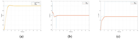
Figure 6.
Comparison of parameter effectiveness. (a) Outputs ; (b) control input ; (c) cost of controls J.
Two control laws were employed to control the system: the SMC and our proposed PISMC. Parameters were tuned so that the two systems had similar settling times. A smaller overshoot occurred in the system using PISMC. Table 1 lists the parameters:

Table 1.
Parameters used for comparison of cost functions.
The simulations in Figure 6 show that the proposed algorithm costs less while keeping similar transient performance. Notably, under the designated parameters, chattering occurs once using the control from SMC. As a result, it can be concluded that our algorithm performs better than the conventional SMC in this specific case.
2.7. PISMC for a Weighted-Control System
Based on the work in [19], we extend our work to a nonlinear system of weighted control, which is usually described by the differential equations
where are the input and output, respectively, and are smooth functions. The gain is unknown, yet assumed to be uniformly bounded.
Assumption 2.
Assume , where and are given constants, time-varying or state-dependent functions [27].
We assume that the control input may enter multiplicatively in the dynamics, and it is natural to choose our estimate of gain as the geometric mean of the above bounds.
Assumption 2 can then be written in the form of
where
Since the PISMC is designed to be robust to the bounded multiplicative uncertainty, as in (43), we call the gain margin of our design, by analogy to the terminology used in linear control. Let
The PISMC is modified from the aforementioned and it has the form:
where the and are defined in (13) and (14), respectively. We summarize the controller design in Theorem 2.
Theorem 2.
Consider the system (41), which satisfies Assumptions 1 and 2. Let the function be specified in (46) with , , and defined in (13), (14), and (15), respectively. Let the gain be designed to satisfy (5). If there exits a such that
then the tracking error as defined in (3) will tend to the neighborhood of zero within a finite time.
Proof.
To prove that PISMC satisfies the sliding conditions, the following Lyapunov function is employed:
If we choose as in (46), then follow similar steps as those in (18):
Finally, let
We obtain
and hence . This ensures that any trajectory converges to the neighborhood around of origin in the phase plane. □
2.8. Comparison of Sliding Surfaces
The design of sliding surface is inherited from [19], whereas the design of control is extended to a weighted-control system. The design of sliding surface in our algorithm extends to the nth order system, and, thus, is considerably different from conventional SMC and PID sliding surface. Table 2 presents the differences.
Table 2.
Conceptual comparison between different control laws.
3. Implementation in a Two-Wheel Vehicle System
This paper extends the design of PISMC controller to a weighted-control system from the work in [19]. Procedures for tuning parameters are also presented in the proceeding section. The third effort of this paper is to implement the proposed control algorithm in a nonlinear system, which is very rare in the literature. A TWVS was built for the implementation and verification of the algorithm. The novelty of this experiment is the employment of its original nonlinear dynamics, instead of commonly used linearized dynamics.
3.1. Model of Two-Wheel Vehicle System
The dynamic equations for the TWVS were derived for analysis and for the controller design. Figure 7 shows the free body diagram of the TWVS.

Figure 7.
(a) Free body diagram of the cart and the pendulum; (b) free body diagram of the wheels
A simplified version of the TWVS is shown at the top of Figure 7a. The shaft of the two wheels goes through the center of mass (cm) of the cart, and a pendulum is installed in the cm of the cart through a hinge. A motor kit is installed on each wheel to drive the wheel. Assume that there is no slip occurred between the wheels and the ground, and no torque exists between the cart and the pendulum. Moreover, this example experiment only considers the longitudinal motion. Therefore, forces and torques in the lateral motion are assumed balanced and not considered.
In order not to distract readers from the main stream of this paper, the detailed derivation of equations of motion is provided in the Appendix A. Notation is defined either in Figure 7 or in the Appendix A. The dynamics of the TWVS are represented as follows:
Define and . The equations of motion of the TWVS can be written as
where
or equivalently,
where .
3.2. Parameter Set-Up of PISMC System
In this section, a numerical simulation and an experiment of PISMC applying to a TWVS are presented. The dynamics of TWVS are defined in (52), and in the simulation, the parameters were selected as kg, kg, kg, m, m, N-m, and N-m. Let . We have and . Set , , , and . The PISMC can be computed from (46).
3.3. Numerical Simulations
3.3.1. Architecture of the Simulation and Experiment
Figure 8 shows the architecture of the simulation and the actual hardware implementation of the PISMC. The measured output signal was compared with the reference signal and the calculations were performed to produce the switching signal and the equivalent signal. The overall control signal (switching signal + equivalent signal) was sent to the motor driving board to control the real system. In the experiment, the motor driving board contained two PIC18F258 microcontrollers. One microcontroller computed the control signal based on the PISMC algorithm, whereas the other handled the readings of sensors. The computational capability of a PIC18F258 microcontroller is actually powerful enough to implement the proposed algorithm. However, due to the inherit complexity and difficulty in the TWVS, the preliminary goal was to achieve the autonomous balance by a simplified structure. Therefore, the experiment focused on the tilt angle control only, described by the equation of in (52). A simple flow chart is shown in Figure 9.

Figure 8.
A block diagram of the overall system.
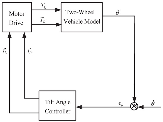
Figure 9.
The experiment focused on the tilt angle control () only, due to the inherit complexity and difficulty in the two-wheel vehicle system (TWVS).
3.3.2. Balance Control Simulation Results
Simulation results are presented in Figure 10, Figure 11 and Figure 12. For the first simulation, Figure 10 shows the system responses of the TWVS balancing with no external disturbances and the initial condition is . We note that the settling time to reach and the error of the PISMC are smaller and converge quicker than that of the conventional SMC. It is evident that the PISMC presented in this paper is effective for the TWVS to reach the desired attitudes around the equilibrium point in short a period. The stability and accuracy are both maintained in the balance simulation.

Figure 10.
Balance response to PISMC without disturbances: (top) angular response; (middle) response of angular rate; (bottom) applied control signals.
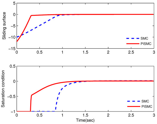
Figure 11.
Switching and sliding signal for PISMC without disturbances: (top) history of sliding surface values; (bottom) history of saturation conditions.

Figure 12.
Balance response to PISMC with disturbances of : (top) angular response; (middle) response of angular rate; (bottom) applied control signals.
For the second simulation, Figure 12 shows the system responses of the TWVS with external disturbances. To examine the disturbance rejection property afforded by the proposed control, we consider to simulate the system with initial condition of , and the system external disturbance is . Figure 11 shows that settles down to the steady state and the amplitude of the errors are smaller. The results also verify that the PISMC is capable of tracking the desired states and the errors converge steadily to the neighborhood of zero.
The performance of the system with the proposed PISMC is better than the use of the SMC controller such that no overshoot, shorter rise time, and shorter settling time were obtained from the proposed controller. The variations of the control efforts are shown in Figure 10 which indicates that the SMC signal is smaller in magnitude and the system settles down in 1.2 s. Several quantitative performance indicators of the attitude tracking qualities for SMC and PISMC controllers are summarized in Table 3. Variations of the sliding signal for SMC and PISMC are illustrated in Figure 10. It shows that magnitudes of the variations are smaller in PISMC. Variations of the sliding surface during the control are illustrated in Figure 10 as well. One notes that the sliding function is when the error signal is not zero. This means that the sliding mode is in the reaching surface up to about 0.92 s, and then arrives the sliding surface. When it reaches to the sliding surface, theoretically it is expected the sliding function to be zero (i.e., ). In practical applications, there are always some small deviations and fluctuations at the output measured variable because of uncertainties and disturbances. Here, the average value of the sliding function is zero . As shown in Figure 10, Figure 11 and Figure 12, we note that these remarkable results are obtained without involving too much control effort.
Table 3.
Time domain specifications.
4. Experiments and Discussion
4.1. The TWVS Platform
In this study, an experimental TWVS was developed as the experimental platform for gathering data to simulate and verify the proposed controller design. A picture of the TWVS is shown in Figure 13. The TWVS was equipped with a microchip (PIC 18F258)-based onboard computer module which was responsible for the data processing and the autonomous control. The main onboard electronic sensor was the self-developed IMU which consisted of the gyroscope and the accelerometer circuit. They were used to collect data from system identification and to output commands for automatic balance. The main control system was composed of the Borland C++ Builder.

Figure 13.
Onboard computer module of the two-wheel vehicle system.
4.2. Attitude Sensors
In general, the orientation of the inertial measurement unit (IMU) is derived from the inertial sensors, i.e., accelerometer and gyroscope sensors. All these sensors provide analog signals, so an analog-to-digital converter (ADC) is required to acquire the data. Therefore, the PIC18F258 made by Microchip Technology, with 8-channel 10-bit ADC, was used. In order to increase the computational efficiency and to perform the data fusion algorithm, microchips (PIC 18F258) served as the processing units of the low-cost IMU, and they communicated with each other through the built-in RS232 bus. The configuration of this self-developed IMU is depicted in Figure 14. This self-developed, low-cost IMU was used to offer attitudes and angular rates for the onboard computer module. The outputs of IMU were Euler angles, angular rates, and accelerations. Although the IMU performs well in normal conditions, its outputs always suffer from unpredictable errors such as moving due to the motor vibrations. The chassis on the TWVS induced vibrations and affected the onboard hardware to some extent. Without proper installation, the IMU probably gives inapplicable outputs. Therefore, vibration isolation or reduction became an important issue for our IMU on a moving platform. Some vibration reduction materials were tested and finally a kind of sound deadening sheet for cars was chosen. The IMU was surrounded by several layers of the sound deadening sheet and then cased into a box.
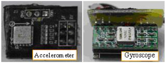
Figure 14.
Attitude sensors: (left) accelerometer; (right) gyroscope.
4.3. Balance Control Experiment Results
For the first experiment with no external disturbances, Figure 15 shows the TWVS tracking responses using the proposed PISMC and the conventional SMC. In experimental results, the original tilt angle was approximately degrees, and the tilt rate was approximately degrees/s. Comparing the top left plot (PISMC) to the top right plot (SMC), one notes that the tilt angle result of the proposed PISMC controller had no overshoot, shorter rise time, and shorter settling time than that of the conventional SMC controller. Importantly, the experimental result shows that the PISMC held balance well for the developed TWVS. The results of the second TWVS experiment with external disturbances are shown in Figure 16, which shows that the output of tilt angle by the PISMC can be tracked well to follow the desired angle. The robustness of the TWVS with the PISMC is better than that of the conventional SMC. It also demonstrates that the PISMC can give reasonable angle output of the tilt motion in experiments. Comparing the PISMC results with the SMC results, the PISMC has smaller oscillation, smaller overshoot, shorter rise time, and shorter settling time than the conventional SMC. The results of the TWVS experiments validate the balance control capability of the PISMC.

Figure 15.
Experimental results of TWVS without disturbances: (left) SMC is implemented; (right) PISMC is implemented.

Figure 16.
Experimental results of TWVS with disturbances: (left) SMC is implemented; (right) PISMC is implemented.
5. Conclusions
This paper presents a generalized proportional-integral sliding mode control (PISMC) method and the design of the associated controls. Our previous work generalized the PISMC to an nth order, unweighted-control system with only two parameters to tune. This paper extends the work to an nth order, weighted-control system. The bounds of dynamic variation, usually including state perturbations and disturbances, were employed to design the associated controller. The advantage of this approach is to avoid measuring the uncertainties. A systematic procedure to tune parameters was analyzed and proposed. Numerical simulations of a nonlinear system are presented to demonstrate the validity of the procedure. Robustness of the proposed algorithm is discussed, and the performance is shown to be better than a conventional SMC under certain parameters through the comparison of costs. These examples also demonstrate that the presence of one more parameter from the integral part brings one more degree of freedom with which to tune the system. In addition, the design of a balance control system for a TWVS is presented to validate the algorithm. The simulation results show that the PISMC autonomously balances the TWVS effectively in both disturbed and undisturbed circumstances, validating the robustness of the algorithm. The performance of the PISMC is also better than that of the conventional SMC. The balance control experiments of the developed TWVS yielded encouraging results that validate the feasibility and the effectiveness of the proposed PISMC controller. The successful implementation of the proposed PISMC using the original nonlinear dynamics potentially extends the applications of the PISMC to various nonlinear and emerging systems.
Author Contributions
Formal analysis, C.-H.L.; Investigation, C.-H.L.; Resources, F.-Y.H.; Supervision, F.-Y.H.; Validation, C.-H.L.; Writing—original draft, C.-H.L.; Writing—review & editing, F.-Y.H. All authors have read and agreed to the published version of the manuscript.
Funding
Taiwan Ministry of Technology and Science with grant number NSC 97-2221-E-006-235-MY3; NCSIST with grant number MOST 106-2623-E-032-001-D; National Space Organization with grant number NSPO-S-109133.
Acknowledgments
The authors would like to dedicate this paper to the late Fei-Bin Hsiao for his precious comments on this work.
Conflicts of Interest
The authors declare no conflict of interest.
Appendix A. Derivation of Dynamic Model
First, consider the dynamics of the left wheel. All notations denoted by subscripts of L and R are associated with the the left and right wheels, respectively. Let be the contact point with the ground; be the friction; be the normal force by the ground; and be the forces exerted by the cart; be the mass of the wheel; be the weight; be the controlling torque provided by the motor; and R be the radius of the two wheels.
The dynamic equations of the wheels in the cart-body-fixed frame are shown as follows
where is the moment of inertia of the wheel and is the rolling angle of the wheel. A similar process can be applied to the right wheel and yields
The assumption of no slipping leads to and . Assume the two wheels are identical. Then , , , . Notably, is defined positive to have the TWVS move toward
The dynamics of the cart is given as follows:
where M is the mass of the cart. Since longitudinal forces are assumed to be exerted passing through the cm and lateral forces are balanced, there is no equation for torques. This also implies that the cart-body-fixed frame does not rotate and it is, hence, coincident with the inertial frame.
The equations of the pendulum’s translation are derived with respect to the cm of the pendulum, whereas the equation of the rotation is derived with respect to the lower tip of the pendulum for convenience, where the pendulum is linked to the cart. Therefore, the equations of motion are obtained by [29]
where m is the mass of the pendulum; is the moment of inertia about the pendulum cm. Moreover, is the position vector pointing from the tip to the pendulum cm, and is the acceleration of the pendulum cm. The two terms can be found by
where l is the half length of the pendulum and is the acceleration of the cart. Expanding (A4) through (A6) yields (49) and
References
- Utkin, V.I. Variable structure with sliding mode: A survey. IEEE Trans. Autom. Control. 1977, 22, 212–222. [Google Scholar] [CrossRef]
- Sira-Ramirez, H.; Zribi, M.; Ahmad, S. Dynamical sliding mode control approach for vertical flight regulation in helicopters. IEE Proc. Control Theory Appl. 1994, 194, 19–24. [Google Scholar] [CrossRef]
- Utkin, V.I.; Jingxin, S. Integral sliding mode in systems operating under uncertainty conditions. In Proceedings of the 35th Conference on Decision and Control, Kobe, Japan, 13 December 1996; pp. 4591–4596. [Google Scholar]
- Baik, I.C.; Kim, K.H.; Youn, M.J. Robust nonlinear speed control of PM synchronous motor using boundary layer integral sliding mode control technique. IEEE Trans. Control Syst. Technol. 2000, 8, 47–54. [Google Scholar] [CrossRef]
- Lin, C.J.; Chen, C.K.; Li, K.S. Extended sliding-mode control for the tracking problem of a rotational inverted pendulum. J. Chin. Soc. Mech. Eng. 2003, 24, 277–282. [Google Scholar]
- Hess, R.A.; Wells, S.R. Sliding mode control applied to reconfigurable flight control design. J. Guid. Control Dyn. 2003, 26, 452–462. [Google Scholar] [CrossRef]
- Rafimanzelat, M.R.; Yazdanpanah, M.J. A novel low chattering sliding mode controller. In Proceedings of the 5th Asian Control Conference, Melbourne, Victoria, Australia, 20–23 July 2004; Volume 3, pp. 1958–1963. [Google Scholar]
- Niu, Y.; Ho, D.W.C.; Lam, J. Robust integral sliding mode control for uncertain stochastic systems. Automatica 2005, 41, 873–880. [Google Scholar] [CrossRef]
- Koshkouei, A.J.; Burnham, K.J.; Zinober, A.S.I. Dynamic sliding mode control design. IEE Proc. Control Theory Appl. 2005, 152, 392–396. [Google Scholar] [CrossRef]
- Bouabdallah, S.; Siegwart, R. Backstepping and sliding mode techniques applied to an indoor micro quad-rotor. In Proceedings of the IEEE International Conference on Robotics and Automation, Barcelona, Spain, 18–22 April 2005; pp. 2259–2264. [Google Scholar]
- Chen, C.A.; Chiang, H.K.; Lin, B.R. The novel adaptive sliding mode position control synchronous reluctance motor drive. J. Chin. Soc. Mech. Eng. 2008, 29, 241–247. [Google Scholar]
- Park, S.; Tan, C.W.; Kim, H.; Hong, S.K. Oscillation control algorithms for resonant sensors with applications to vibratory gyroscopes. Sensors 2009, 9, 5952–5967. [Google Scholar] [CrossRef] [PubMed]
- Waslander, S.L.; Hoffmann, G.M.; Jang, J.S.; Tomlin, C.J. Multi-agent quad-rotor test-bed control design: Integral sliding mode vs. reinforcement learning. In Proceedings of the IEEE/RSJ International Conference on Intelligent Robots and Systems, Edmonton, AB, Canada, 2–6 August 2005; pp. 468–473. [Google Scholar]
- Soylu, S.; Buckham, B.; Podhorodeski, R. MIMO sliding-mode and H∞ controller design for dynamic coupling reduction in underwater-manipulator systems. Trans. Can. Soc. Mech. Eng. 2009, 33, 731–744. [Google Scholar] [CrossRef]
- Nawawi, S.; Ahmad, M.; Osman, J.; Husain, A.; Abdollah, M. Controller Design for Two-wheels Inverted Pendulum Mobile Robot Using PISMC. In Proceedings of the 4th Student Conference on Research and Development, Shah Alam, Malaysia, 27–28 June 2006; pp. 194–199. [Google Scholar]
- Nawawi, S.; Osman, J.; Ahmad, M. A PI Sliding Mode Tracking Controller with Application to a 3-DOF Direct drive Robot Manipulator. In Proceedings of the TENCON 2004—2004 IEEE Region 10 Conference, Chiang Mai, Thailand, 21–24 November 2004; Volume 4, pp. 455–458. [Google Scholar]
- Sam, M.; Osman, J.; Ghani, R. Proportional integral sliding mode control of a quarter car active suspension. In Proceedings of the TENCON 2002—2002 IEEE Region 10 Conference, Beijing, China, 28–31 October 2002; Volume 3, pp. 1630–1633. [Google Scholar]
- Sam, Y.; Suaib, N.; Osman, J. Hydraulically Actuated Active Suspension System with PISMC. WSEAS Trans. Syst. Control 2008, 3, 859–868. [Google Scholar]
- Lin, C.H.; Jan, S.S.; Hsiao, F.B. Autonomous hovering of an experimental unmanned helicopter system with proportional-integral sliding mode control. ASCE J. Aerosp. Eng. 2011, 243, 338–348. [Google Scholar] [CrossRef]
- Tho, H.D.; Tasaki, R.; Kaneshige, A.; Miyoshi, T.; Terashima, K. Robust Sliding Mode Control with Integral Sliding surface of an underactuated rotary hook system. In Proceedings of the 2017 IEEE International Conference on Advanced Intelligent Mechatronics (AIM), Munich, Germany, 3–7 July 2017; pp. 998–1003. [Google Scholar]
- Pan, Y.; Yang, C.; Pan, L.; Yu, H. Integral Sliding Mode Control: Performance, Modification, and Improvement. IEEE Trans. Ind. Inform. 2018, 14, 3087–3096. [Google Scholar] [CrossRef]
- Abbasi, S.; Kallu, K.; Lee, M. Efficient Control of a Non-Linear System Using a Modified Sliding Mode Control. Appl. Sci. 2019, 9, 1284. [Google Scholar] [CrossRef]
- Monsalve-Rueda, M.; Candelo-Becerra, J.; Hoyos, F. Dynamic Behavior of a Sliding-Mode Control Based on a Washout Filter with Constant Impedance and Nonlinear Constant Power Loads. Appl. Sci. 2019, 9, 4548. [Google Scholar] [CrossRef]
- Zheng, X.; Jian, X.; Du, W.; Cheng, H. Nonlinear Integral Sliding Mode Control for a Second Order Nonlinear System. J. Control Sci. Eng. 2015, 2015, 218198 . [Google Scholar] [CrossRef]
- Cairone, F.; Gagliano, S.; Bucolo, M. Experimental study on the slug flow in a serpentine microchannel. Exp. Therm. Fluid Sci. 2016, 76, 34–44. [Google Scholar] [CrossRef]
- Schembri, F.; Sapuppo, F.; Bucolo, M. Experimental classification of nonlinear dynamics in microfluidic bubbles’ flow. Nonlinear Dyn. 2012, 67, 2807–2819. [Google Scholar] [CrossRef]
- Slotine, J.J.E.; Li, W. Applied Nonlinear Control; Prentice-Hall: Englewood Cliffs, NJ, USA, 1991. [Google Scholar]
- Vaidyanathan, S.; Lien, C.H.E. Applications of Sliding Mode Control in Science and Engineering; Springer: New York, NY, USA, 2017. [Google Scholar]
- Hibbeler, R.C. Engineering Mechanics: Dynamics, 14th ed.; Pearson: New York, NY, USA, 2016. [Google Scholar]


© 2020 by the authors. Licensee MDPI, Basel, Switzerland. This article is an open access article distributed under the terms and conditions of the Creative Commons Attribution (CC BY) license (http://creativecommons.org/licenses/by/4.0/).