The Effects of Stress on Second Harmonics in Plate-Like Structures

Abstract

Cumulative second harmonic of ultrasonic guided waves is considered to have great application potential in evaluating internal stress of structures. One difficulty with the application is the diversity and complexity of modal response to the stress change in waveguide. At present, there is a lack of relevant theoretical studies and experimental results to guide the applications. In this article, a method is proposed to characterize the amplitude change of cumulative second harmonic mode in a plate under stress through calculating the amplitude coefficient, which can be acquired based on mode shape analysis. The steel plate is taken as an example to demonstrate the analysis method. Experimental studies are presented with results consistent with the theoretical predictions. The results of this study indicate that the amplitudes of different cumulative second harmonic modes may increase or decrease monotonically with the change of stress. Therefore, when the phenomenon of modes mixing occurs in the waveguide, it is necessary to analyze and predict the amplitude of selected cumulative second harmonic mode with the change of stress in advance; otherwise, wrong results may be obtained. The method and conclusions proposed in this paper can also be applicable to waveguide of arbitrary cross-section and have universality.

1. Introduction

When the ultrasonic waves propagate in the solid medium, because of the anharmonicity of the crystal structure and the existence of the internal micro defects (micro cracks, stress concentration, etc.), the ultrasonic waves will have “distortion” in the process of propagation, showing a strong nonlinear effect. The nonlinear phenomena are specifically manifested in that the received signal will generate high-order harmonics in addition to the original fundamental frequency signal. The high-order harmonics contain the information that is difficult to be detected by traditional ultrasonic technologies, such as the micro defects in the structure and the material characteristics. Nonlinear ultrasonic technology applies acoustic means to extract the high-order harmonics in the received signal and calculates the unique ultrasonic nonlinear parameter. Nonlinear parameter can be used to quantify the change of material properties and the degree of damage inside the structure, so as to realize the health monitoring and evaluation of the structure [1,2,3,4,5,6,7].

In recent years, nonlinear ultrasonic guided waves have drawn increasing attention in the field of structural stress detection, as a result of their advantages of traditional ultrasonic guided waves [8,9,10,11,12,13], high sensitivity, and unique characteristics of determining the internal state of structure. Bartoli [14,15] studied the application of nonlinear guided waves to the stress detection of pre-stressed steel bars in concrete structures and found that the contact stress between any strand and adjacent strand was closely related to the nonlinear effect of guided waves. Liu [16,17] proved that the nonlinear surface waves can be used to detect the residual stress on the surface of aluminum alloy. Yan [18,19] built a residual stress prediction model by exploring the nonlinear characteristics of the metal material in the process of tension and compression.

In addition to the progress of applications, there is also a good development in theoretical researches. Auld [20] introduced an efficient technique based on the mode expansion method, to obtain second harmonic modal expression. Deng [21,22,23] investigated the nonlinear phenomenon of ultrasonic Lamb waves in the elastic plate by using second-order perturbation approximation. Deng concluded that the cumulative second harmonic exists under some conditions. The cumulative second harmonic means that second harmonic modal amplitude increases with the increase of propagation distance. De Lima and Hamilton [24,25] arrived at the conclusion that the cumulative effect of second harmonic takes place only when the phase-velocity matching between fundamental mode and second harmonic mode is satisfied and the power flow from fundamental mode to second harmonic mode is not zero. Chillara and Lissenden [26] further analyzed the types of cumulative second harmonic modes in the plate and proposed that if a second harmonic mode whose amplitude can be accumulated in the plate is to be generated, the second harmonic mode must be a symmetric mode. Srivastava and Di Scalea [27] theoretically studied the symmetry characteristics of nonlinear Rayleigh–Lamb waves in plate and explained the reason behind the absence of antisymmetric modes at the cumulative second harmonic. Lee [28,29] proposed another condition for the generation of the cumulative second harmonic, that is, the group velocity of the fundamental mode should be equal to the group velocity of second harmonic mode. However, Deng [30] further proved both analytically and experimentally that, as long as the two aforementioned conditions (phase-matching and non-zero power flux) are satisfied, the cumulative second harmonic can be generated, even though the group velocity matching condition is not satisfied. Liu Yang [31,32] calculated the magnitude of energy flow between different excitation and reception modes in aluminum plate and proposed to select the optimal combination of excitation and reception modes through the magnitude of energy flow.

Previous researches have made a comprehensive theoretical framework for the generation of cumulative second harmonic modes, and to a certain extent, the mode pair of fundamental mode and second harmonic mode is determined. In the current studies of applying nonlinear ultrasonic guided waves to detect structural stress, second harmonic mode is selected from the mode pairs meet the conditions, and the corresponding relative nonlinear parameter is calculated. Then the stress change of the structure is characterized according to the change of the relative nonlinear parameter. Due to the multi-modal characteristics of ultrasonic guided waves, the mode pair which satisfy the conditions is not unique, and there may be possibly more cumulative second harmonic modes. The changes of the amplitudes of different second harmonic modes with stress are not necessarily the same, and that will lead to the different trends of the relative nonlinear parameters. In particular, when different second harmonic modes are overlapped, the calculation of relative nonlinear parameter will be affected, and wrong experimental results may be obtained. So far, research on the law of the amplitude of the second harmonic mode change with stress has not been carried out. This article puts forward a clear and definite method to determine the response law of the amplitude of each second harmonic mode in plate with the change of stress. The research results can provide the basis for the selection of suitable second harmonic mode for experiment and subsequent application. A steel plate is used as a model for simulation and physical verification, and simulation results are in agreement with the experimental results. The results demonstrate that the change trends of amplitudes of different second harmonic modes with stress are not the same, which are monotonic increasing or decreasing. As a result, the variation of second harmonic modal amplitude with stress should be considered and predicted in advance, when the nonlinear ultrasonic guided waves are selected for stress detection in plate.

2. Theoretical Basis

2.1. Nonlinear Ultrasonic Guided Waves

When the elastic solid deforms, the strain energy will be produced in the solid. The relationship between the strain energy, $W$, and the second Piola–Kirchhoff stress tensor, $T_{ij}$, is given by the following:

$$T_{ij}=\frac{\partial W}{\partial E_{ij}}$$

(1)

where $E_{ij}=\frac{1}{2}\left(u_{i,j}+u_{j,i}+u_{k,i}{u}_{k,j}\right)$, $u_{i,j}=\frac{\partial u_i}{\partial x_j}$, $u$ is the particle displacement vector, $x$ is the material spatial coordinates, and $i,j,k=x,y,z$. Substitute the widely used constitutive model $W$ that was proposed by Landau and Lifshitz [33,34] into Equation (1), and the expression of $T_{ij}$ about $E_{ij}$ is as follows:

$$T_{ij}=\lambda E_{kk}{\delta }_{ij}+2\mu E_{ij}+{\delta }_{ij}\left(C{E}_{kk}{E}_{ll}+B{E}_{kl}{E}_{lk}\right)+2B{E}_{kk}{E}_{ij}+A{E}_{jk}{E}_{ki}$$

(2)

where $\lambda ,\mu$ are Lame’s constants, $A,B,C$ are the third-order elastic constants, ${\delta }_{ij}$ is the Kronecker delta, and $T_{ij}$ can be divided into two parts, $T_{ij}{}^L$ and $T_{ij}{}^{NL}$:

$$T_{ij}{}^L=\lambda u_{k,k}{\delta }_{ij}+\mu (u_{i,j}+u_{j,i})$$

(3)

$$T_{ij}{}^{NL}=T_{ij}(E_{ij})-T_{ij}{}^L$$

(4)

where $T_{ij}{}^L$ and $T_{ij}{}^{NL}$ represent the stress tensor due to the linear and nonlinear parts of the strain tensor.

The nonlinear wave equation of ultrasonic waves propagates in homogeneous isotropic hyper-elastic solid [35]:

$$\left(\lambda +\mu \right)u_{j,ji}+\mu u_{i,jj}+f_i=\rho {\ddot{u}}_i$$

(5)

where

$$\begin{gathered} f_i=\left(\mu +\frac{A}{4}\right)\left(u_{l,kk}{u}_{l,i}+u_{l,kk}{u}_{i,l}+2u_{i,lk}{u}_{l,k}\right)+\left(\lambda +\mu +\frac{A}{4}+B\right)\left(u_{l,ik}{u}_{l,k}+u_{k,lk}{u}_{i,l}\right) \\ +\left(\lambda +B\right)\left(u_{i,kk}{u}_{l,l}\right)+\left(\frac{A}{4}+B\right)\left(u_{k,lk}{u}_{l,i}+u_{l,ik}{u}_{k,l}\right)+\left(B+2C\right)\left(u_{k,ik}{u}_{l,l}\right) \end{gathered}$$

(6)

where $f_i$ represents the body force, which includes all nonlinear terms. The stress-free boundary condition is as follows:

$$S_{ij}{}^L{n}_j=-S_{ij}{}^{NL}{n}_j \mathrm{on} S$$

(7)

where $n_j$ is the unit vector normal to the surface of the waveguide, and $S$ is the surface of the waveguide. $S_{ij}{}^L$ and $S_{ij}{}^{NL}$ represent the linear and nonlinear parts of the surface force $S_{ij}$ on the material, and the expressions are as follows:

$$S_{ij}{}^L=T_{ij}{}^L$$

(8)

$$\begin{gathered} S_{ij}{}^{NL}=\left(\frac{\lambda }{2}{u}_{k,l}{u}_{k,l}+C{u}_{k,k}{u}_{l,l}\right){\delta }_{ij}+B{u}_{k,k}{u}_{j,i}+\frac{A}{4}{u}_{j,k}{u}_{k,i}+\frac{B}{2}\left(u_{k,l}{u}_{k,l}+u_{k,l}{u}_{l,k}\right){\delta }_{ij} \\ +\left(\lambda +B\right)u_{k,k}{u}_{i,j}+\left(\mu +\frac{A}{4}\right)\left(u_{i,k}{u}_{j,k}+u_{k,i}{u}_{k,j}+u_{i,k}{u}_{k,j}\right) \end{gathered}$$

(9)

The perturbation method is used to get the particle displacement. Assume the material particle displacement is as follows:

$$u_i=u_i{}^{\left(1\right)}+u_i{}^{\left(2\right)}$$

(10)

where $u_i{}^{\left(1\right)}$ and $u_i{}^{\left(2\right)}$ are the displacements caused by material linearity and nonlinearity, respectively; and the values of $u_i{}^{\left(1\right)}$ and $u_i{}^{\left(2\right)}$ are the linear sum of the amplitudes of the correlated guided waves modes, $u_i{}^{\left(1\right)}>>u_i{}^{\left(2\right)}$. Substitute Equation (10) into Equations (5) and (7), and the equation of motion and boundary condition of nonlinear displacement components are obtained [36] as follows:

$$\left(\lambda +\mu \right)u_{j,ji}{}^{\left(2\right)}+\mu u_{i,jj}{}^{\left(2\right)}+f_i{}^{\left(1\right)}=\rho {\ddot{u}}_i{}^{\left(2\right)}$$

(11)

$$S_{ij}{{}^L}^{\left(2\right)}{n}_j=-S_{ij}{{}^{NL}}^{\left(1\right)}{n}_j \mathrm{on} S$$

(12)

where $f_i{}^{\left(1\right)}=f_i\left(u_i{}^{\left(1\right)}\right)$, $S_{ij}{{}^L}^{\left(2\right)}=S_{ij}{}^L\left(u_i{}^{\left(2\right)}\right)$, and $S_{ij}{{}^{NL}}^{\left(1\right)}=S_{ij}{}^{NL}\left(u_i{}^{\left(1\right)}\right)$. If we solve Equations (11) and (12), $u_i{}^{\left(2\right)}$ can be obtained, which represents the particle displacement caused by second harmonic modes.

2.2. Amplitude Coefficient of Second Harmonic Mode

Presume the waveguide cross-section is the y-z plane, and the wave propagation direction is x direction. The expression of $u_i{}^{\left(2\right)}$ [20,37] is as follows:

$$u_i{}^{\left(2\right)}={\displaystyle \sum _{n=1}^N{A}_n(x)u_n}{e}^{-i2\omega t}$$

(13)

where $N$ is the number of modes with an angular frequency of $2\omega$, $n$ represents the nth mode at the angular frequency $2\omega$, $u_n$ is the mode shape of the nth mode, and $A_n(x)$ is the amplitude function of the nth mode. The expression of $A_n(x)$ is as follows:

$$A_n(x)=\{\begin{array}{c}\frac{f_n{}^{surf}+f_n{}^{vol}}{2P_{nn}(k_n{}^{\ast }-2k)}\sin \left(\frac{1}{2}\left(k_n{}^{\ast }-2k\right)x\right)u_n\left(x\right)e^{i\left(\left(1/2\right)\left(2k+k_n{}^{\ast }\right)x-2\omega t\right)},k_n{}^{\ast }\ne 2k_1\\ \frac{f_n{}^{surf}+f_n{}^{vol}}{4P_{nn}}x{u}_n\left(x\right)e^{2i(kx-\omega t)},k_n{}^{\ast }=2k_1\end{array}$$

(14)

where

$$P_{nn}=-\frac{1}{2}{\displaystyle \underset{\mathsf{\Omega }}{\int }(v_n{{}^T}^{\ast }\cdot T_{ij(n)}{}^L)}\cdot n_{x}d\mathsf{\Omega }$$

(15)

$$f_n^{surf}={\displaystyle \underset{S}{\int }(v_n{{}^T}^{\ast }\cdot S_{ij(1)}{}^{NL})}\cdot \overrightarrow{n}dS$$

(16)

$$f_n^{vol}={\displaystyle \underset{\mathsf{\Omega }}{\int }{v}_n{{}^T}^{\ast }\cdot f_{i(1)}}d\mathsf{\Omega }$$

(17)

where $f_n^{surf}$ and $f_n^{vol}$ represent the power flux from the primary excitation mode to the nth secondary mode through the surface and the volume of the waveguide, respectively. $P_{nn}$ represents the average power flow along the wave propagation direction. $k_1$ is the wavenumber of the primary excitation mode, $k_n{}^{\ast }$ is the complex conjugate of wavenumber of the nth secondary mode, $v_n$ is the particle velocity of the nth secondary mode, $T_{ij(n)}{}^L=T_{ij}{}^L(u_n)$, $S_{ij(1)}{}^{NL}=S_{ij}{}^{NL}(u_n{}^{\left(1\right)})$, and $f_{i(1)}=f_i(u_n{}^{\left(1\right)})$. $u_n{}^{\left(1\right)}$ is the mode shape of the primary excitation mode corresponding to the nth secondary mode. $n_x$ is the unit vector in the wave propagation direction. $\overrightarrow{n}$ is the unit vector normal to the surface of the waveguide, $S$, and $\mathsf{\Omega }$ is the waveguide cross-section area.

The amplitude coefficient of the second harmonic mode, ${\overline{A}}_n(x)$, can be defined as follows:

$${\overline{A}}_n(x)=\{\begin{array}{c}\left|\frac{f_n{}^{surf}+f_n{}^{vol}}{2P_{nn}(k_n{}^{\ast }-2k)}\sin \left(\frac{1}{2}\left(k_n{}^{\ast }-2k\right)x\right)\right|,k_n{}^{\ast }\ne 2k_1\\ \left|\frac{f_n{}^{surf}+f_n{}^{vol}}{4P_{nn}}x\right|,k_n{}^{\ast }=2k_1\end{array}$$

(18)

where ${\overline{A}}_n(x)$ determines how large the amplitude of the second harmonic mode is [37]. Equation (18) shows that, for the mode with an angular frequency of $2\omega$, the amplitude will increase with the rise of the propagation distance only when the following two conditions are satisfied:

• Phase matching: $k_n{}^{\ast }=2k_1$;
• Non-zero power flux: $f_n{}^{surf}+f_n{}^{vol}\ne 0$.

At present, in the researches and applications of nonlinear ultrasonic guided waves, group velocity matching does not represent a necessary requirement for cumulative second-harmonic generation. For this reason, only phase matching and power transfer are considered in detail in this article.

The amplitude coefficient of second harmonic mode, ${\overline{A}}_n(x)$, is directly related to the mode shapes of fundamental mode and second harmonic mode. The relevant formulas are as follows:

$$v_n=-i2\omega u_n$$

(19)

$$T_{ij(n)}{}^L=T_{ij}{}^L(u_n)=\lambda (E_1\cdot a)I_{3\times 3}+\mu (b+b^T)$$

(20)

$$\begin{gathered} S_{ij(1)}{}^{NL}=S_{ij}{}^{NL}(u_n{}^{\left(1\right)})=(\frac{\lambda }{2}(c^T\cdot c)+C{(E_1\cdot c)}^2)I_{3\times 3}+B(E_1\cdot c)d^T+\frac{A}{4}(d^T\cdot d^T) \\ +\frac{B}{2}(c^T\cdot c+c^T\cdot E_2\cdot c)I_{3\times 3}+(\lambda +B)(E_1\cdot c)d+(\mu +\frac{A}{4})(d\cdot d^T+d^T\cdot d+d\cdot d) \end{gathered}$$

(21)

$$\begin{gathered} f_{i(1)}=f_i(u_n{}^{\left(1\right)})=(\mu +\frac{A}{4})(e\cdot l+d\cdot l+2m\cdot c)+(\lambda +\mu +\frac{A}{4}+B)(h^T\cdot c+d\cdot E_3\cdot g) \\ +(\lambda +B)(E_1\cdot c\cdot E_4\cdot f)+(\frac{A}{4}+B)(d^T\cdot E_3\cdot g+h^T\cdot E_2\cdot c)+(B+2C)(E_1\cdot g\cdot E_3\cdot c) \end{gathered}$$

(22)

where $a=\left[\begin{array}{c}\frac{\partial }{\partial x}{u}_n\\ \frac{\partial }{\partial y}{u}_n\\ \frac{\partial }{\partial z}{u}_n\end{array}\right]$, $b=\left[\begin{array}{ccc}\frac{\partial }{\partial x}{u}_n& \frac{\partial }{\partial y}{u}_n& \frac{\partial }{\partial z}{u}_n\end{array}\right]$, $c=\left[\begin{array}{c}\frac{\partial }{\partial x}{u}_n{}^{\left(1\right)}\\ \frac{\partial }{\partial y}{u}_n{}^{\left(1\right)}\\ \frac{\partial }{\partial z}{u}_n{}^{\left(1\right)}\end{array}\right]$, $d=[\begin{array}{ccc}\frac{\partial }{\partial x}{u}_n{}^{\left(1\right)}& \frac{\partial }{\partial y}{u}_n{}^{\left(1\right)}& \frac{\partial }{\partial z}{u}_n{}^{\left(1\right)}\end{array}]$, $e=\left[\begin{array}{c}\frac{\partial }{\partial x}{u}_n{{}^{\left(1\right)}}^T\\ \frac{\partial }{\partial y}{u}_n{{}^{\left(1\right)}}^T\\ \frac{\partial }{\partial z}{u}_n{{}^{\left(1\right)}}^T\end{array}\right]$, $f=\left[\begin{array}{c}\frac{{\partial }^2}{\partial x^2}{u}_n{}^{\left(1\right)}\\ \frac{{\partial }^2}{\partial y^2}{u}_n{}^{\left(1\right)}\\ \frac{{\partial }^2}{\partial z^2}{u}_n{}^{\left(1\right)}\end{array}\right]$, $g=\left[\begin{array}{c}\frac{{\partial }^2}{\partial x^2}{u}_n{}^{\left(1\right)}\\ \frac{{\partial }^2}{\partial x\partial y}{u}_n{}^{\left(1\right)}\\ \frac{{\partial }^2}{\partial x\partial z}{u}_n{}^{\left(1\right)}\\ \frac{{\partial }^2}{\partial y^2}{u}_n{}^{\left(1\right)}\\ \frac{{\partial }^2}{\partial y\partial z}{u}_n{}^{\left(1\right)}\\ \frac{{\partial }^2}{\partial z^2}{u}_n{}^{\left(1\right)}\end{array}\right]$, $h=\left[\begin{array}{ccc}\frac{{\partial }^2}{\partial x^2}{u}_n{}^{\left(1\right)}& \frac{{\partial }^2}{\partial x\partial y}{u}_n{}^{\left(1\right)}& \frac{{\partial }^2}{\partial x\partial z}{u}_n{}^{\left(1\right)}\\ \frac{{\partial }^2}{\partial x\partial y}{u}_n{}^{\left(1\right)}& \frac{{\partial }^2}{\partial y^2}{u}_n{}^{\left(1\right)}& \frac{{\partial }^2}{\partial y\partial z}{u}_n{}^{\left(1\right)}\\ \frac{{\partial }^2}{\partial x\partial z}{u}_n{}^{\left(1\right)}& \frac{{\partial }^2}{\partial y\partial z}{u}_n{}^{\left(1\right)}& \frac{{\partial }^2}{\partial z^2}{u}_n{}^{\left(1\right)}\end{array}\right]$, $l=[\frac{{\partial }^2}{\partial x^2}{u}_n{}^{\left(1\right)}+\frac{{\partial }^2}{\partial y^2}{u}_n{}^{\left(1\right)}+\frac{{\partial }^2}{\partial z^2}{u}_n{}^{\left(1\right)}]$, $m=[\begin{array}{ccccccccc}\frac{{\partial }^2}{\partial x^2}{u}_n{}^{\left(1\right)}& \frac{{\partial }^2}{\partial x\partial y}{u}_n{}^{\left(1\right)}& \frac{{\partial }^2}{\partial x\partial z}{u}_n{}^{\left(1\right)}& \frac{{\partial }^2}{\partial x\partial y}{u}_n{}^{\left(1\right)}& \frac{{\partial }^2}{\partial y^2}{u}_n{}^{\left(1\right)}& \frac{{\partial }^2}{\partial y\partial z}{u}_n{}^{\left(1\right)}& \frac{{\partial }^2}{\partial x\partial z}{u}_n{}^{\left(1\right)}& \frac{{\partial }^2}{\partial y\partial z}{u}_n{}^{\left(1\right)}& \frac{{\partial }^2}{\partial z^2}{u}_n{}^{\left(1\right)}\end{array}]$, $E_1=\left[\begin{array}{ccccccccc}1& 0& 0& 0& 1& 0& 0& 0& 1\end{array}\right]$, $E_2=\left[\begin{array}{ccccccccc}1& 0& 0& 0& 0& 0& 0& 0& 0\\ 0& 0& 0& 1& 0& 0& 0& 0& 0\\ 0& 0& 0& 0& 0& 0& 1& 0& 0\\ 0& 1& 0& 0& 0& 0& 0& 0& 0\\ 0& 0& 0& 0& 1& 0& 0& 0& 0\\ 0& 0& 0& 0& 0& 0& 0& 1& 0\\ 0& 0& 1& 0& 0& 0& 0& 0& 0\\ 0& 0& 0& 0& 0& 1& 0& 0& 0\\ 0& 0& 0& 0& 0& 0& 0& 0& 1\end{array}\right]$, $E_3=\left[\begin{array}{cccccccccccccccccc}1& 0& 0& 0& 1& 0& 0& 0& 1& 0& 0& 0& 0& 0& 0& 0& 0& 0\\ 0& 0& 0& 1& 0& 0& 0& 0& 0& 0& 1& 0& 0& 0& 1& 0& 0& 0\\ 0& 0& 0& 0& 0& 0& 1& 0& 0& 0& 0& 0& 0& 1& 0& 0& 0& 1\end{array}\right]$, $E_4=\left[\begin{array}{ccccccccc}1& 0& 0& 1& 0& 0& 1& 0& 0\\ 0& 1& 0& 0& 1& 0& 0& 1& 0\\ 0& 0& 1& 0& 0& 1& 0& 0& 1\end{array}\right]$, $I$ is the unit matrix.

In the nonlinear ultrasonic experiments, because the change of the amplitude of second harmonic is related to the change of the fundamental signal, the variation of the amplitude of second harmonic cannot be used as the standard to judge the change of material nonlinearity. Therefore, the relative nonlinear parameter, $\beta$, is used to characterize the nonlinearity in the structure. The calculation formula of the relative nonlinear parameter, $\beta$, is as follows:

$$\beta =\frac{A(2\omega )}{A{(\omega )}^2}$$

(23)

where $A(\omega )$ is the amplitude of fundamental frequency signal of received signal, and $A(2\omega )$ is the amplitude of second harmonic of received signal. The magnitude of the relative nonlinear parameter, $\beta$, mainly depends on the amplitude of second harmonic mode. Thus, in the experimental analysis of this paper, the change of the relative nonlinear parameter, $\beta$, is used to characterize the change of the amplitude of the second harmonic mode.

3. Analytical Method of Second Harmonics Under Stress Change

The amplitude coefficient, ${\overline{A}}_n(x)$, under the different stress can be acquired by replacing the related mode shapes $u_n$ and $u_n{}^{\left(1\right)}$ into Equation (18). The mode shapes of ultrasonic guided waves can be solved through the semi-analytical finite element (SAFE) method. By comparing ${\overline{A}}_n(x)$ under the different stress, the response law of the amplitude of second harmonic mode with the stress in plate is obtained.

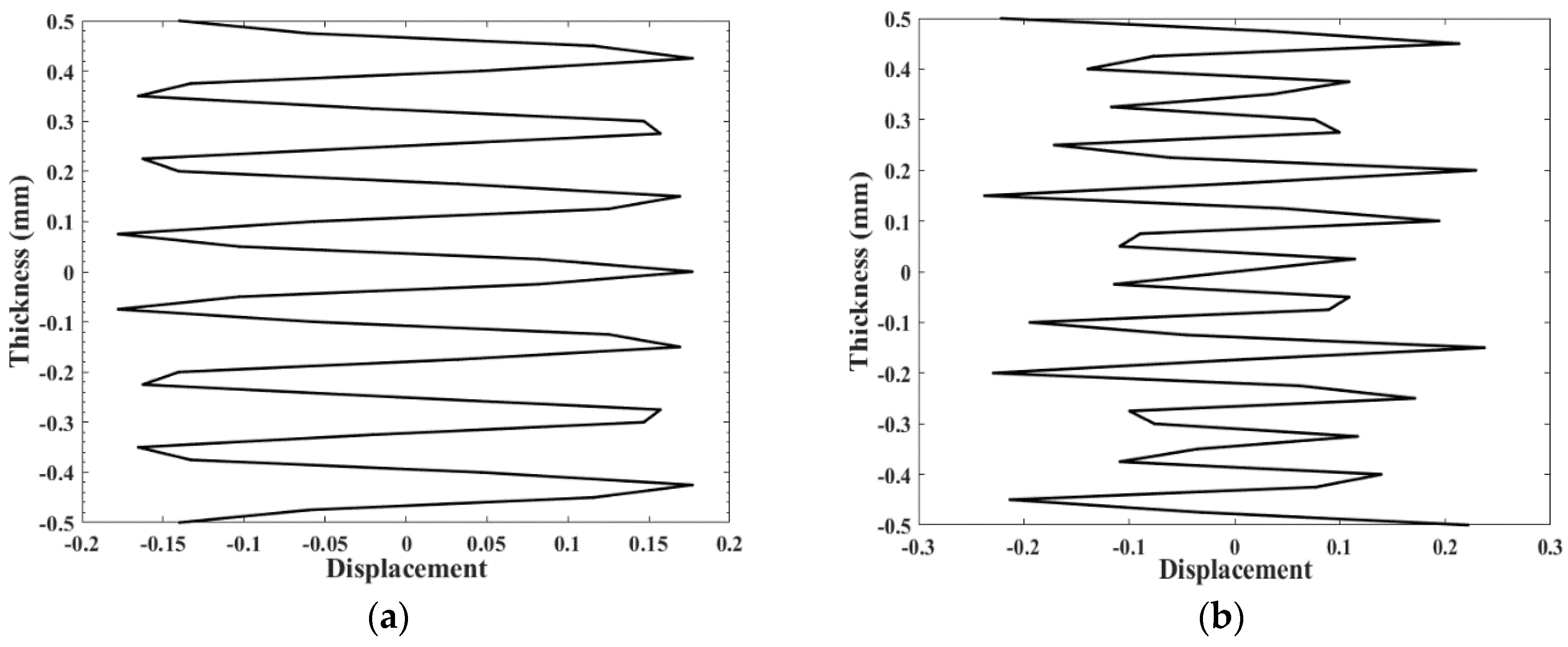
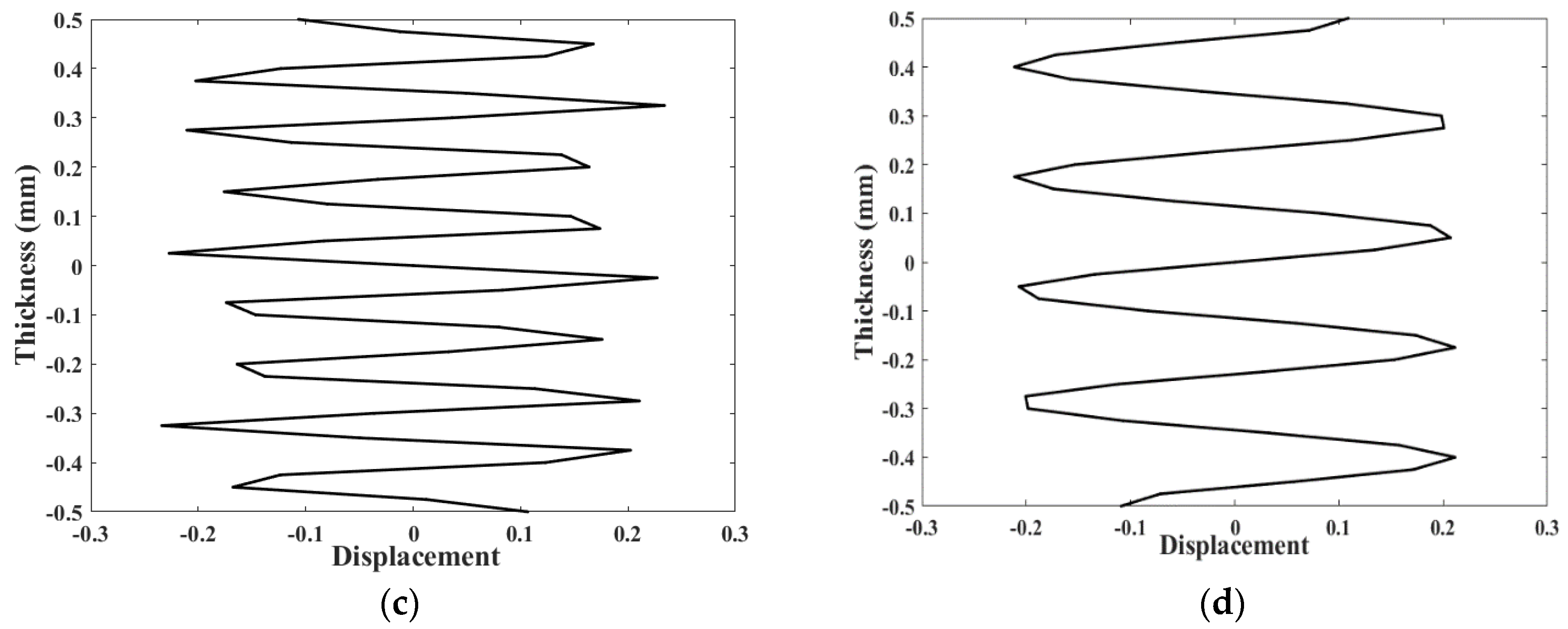
3.1. Mode Shape Calculation

SAFE is a kind of calculation method to solve the mode shapes of ultrasonic guided waves for waveguide with arbitrary cross-section. Through the finite element discretization of the cross-section of the waveguide, the displacement along the wave propagation direction of waveguide is represented by the simple harmonic waves. The cross-section of the waveguide was defined as the y-z plane, and the waves propagate along the x direction. When the cross-section of the waveguide is discretized by finite elements, the displacement of any node in the element can be expressed in the form of shape function, as follows:

$$u_i{}^{(e)}(x,y,z,t)={\left[\begin{array}{c}{\displaystyle \sum _{k=1}^m{N}_k(y,z)U_{xk}}\\ {\displaystyle \sum _{k=1}^m{N}_k(y,z)U_{yk}}\\ {\displaystyle \sum _{k=1}^m{N}_k(y,z)U_{zk}}\end{array}\right]}^{(e)}{e}^{i(kx-\omega t)}=N(y,z)q^{(e)}{e}^{i(kx-\omega t)}$$

(24)

where $m$ is the number of nodes of element, $k$ is the wavenumber, $\omega$ is the angular frequency, $N(y,z)$ is the shape function matrix, and $q^{(e)}$ is the nodal displacements of element. According to Hamiltonian principle, the wave equation of ultrasonic guided waves propagating in the structure can be obtained, which can be transformed into the standard characteristic equation:

$$\left[K_1+ik{K}_2+k^2{K}_3-{\omega }^{2}M\right]u=0$$

(25)

where $K_1$, $K_2$, and $K_3$ are the element stiffness matrix, and $M$ is the mass matrix. Further introduce the stress variable $K_0$, and the expression [15,38] is as follows:

$$\left[K_1+ik{K}_2+k^2\left(K_3+K_0\right)-{\omega }^{2}M\right]u=0$$

(26)

where $K_0=\frac{\sigma }{\rho }M$, and $\sigma$ is the axial stress on waveguide. It should be noted that only the axial load on the waveguide is considered in this article. For each given wave number, the eigenvalue and eigenvector are computed by solving Equation (26). The eigenvalue is the angular frequency, and the eigenvector is the displacement vector of each node in the cross-section, which represents the mode shape of the ultrasonic wave mode under certain stress.

3.2. Analysis of Second Harmonics in Plate

Suppose the model of infinite width free plate is as shown in Figure 1; its cross-section is the y-z plane, and the wave propagation direction is the x direction. A one-dimensional three-nodes element is applied to discretize the cross-section of the plate. Each element has three nodes, and each node has three degrees of freedom, corresponding to the displacement in the coordinate axis direction, as shown in Figure 2.

The thickness of the plate model is 15 mm, the material is defined as steel, and the relevant density, Lame coefficients, and third-order elastic constants of the model are tabulated in

Table 1. Material properties of the plate.

$\mathit{\rho }(\mathit{k}\mathit{g}/{\mathit{m}}^3)$	$\mathit{\lambda }(\mathit{G}\mathit{P}\mathit{a})$	$\mathit{\mu }(\mathit{G}\mathit{P}\mathit{a})$	$\mathit{A}(\mathit{G}\mathit{P}\mathit{a})$	$\mathit{B}(\mathit{G}\mathit{P}\mathit{a})$	$\mathit{C}(\mathit{G}\mathit{P}\mathit{a})$
7932	116	83	−340	−647	−17

[39]. According to Equation (25), the dispersion curves of phase velocity and group velocity of Lamb waves in stress-free steel plate can be obtained by MATLAB software. The dispersion curves are shown in Figure 3 and Figure 4. In Figure 3 and Figure 4, $C_p$ ($C_p=\omega /k$) is the phase velocity of ultrasonic guided wave mode, $C_g$ ($C_g=d\omega /dk$) is the group velocity of ultrasonic guided wave mode, and $fd$ is the frequency-thickness product. It can be seen from Figure 3 and Figure 4 that there are many modes at the same frequency, and the number of modes increases with the increase of frequency, which reflects the multi-modal characteristics of ultrasonic guided waves. Each point in the dispersion curve represents a mode at the certain frequency. Through the dispersion curve, the phase velocity, group velocity, and mode shape of any mode can be obtained.

Without loss of generality, the excitation signal frequency of 2.5 MHz is used in the following study, to facilitate experimental verification of the proposed method with the 2.5 and 5 MHz transducers in the laboratory. According to the phase matching and cumulative second harmonic mode that should be a symmetric mode, all the mode pairs that may generate cumulative second harmonic are selected, the mode shapes of each mode pairs are obtained, and the value of $f_n{}^{surf}+f_n{}^{vol}$ is calculated. The relevant values are shown in

Table 2. Parameters of mode pairs.

Number of Mode Pair	Frequency-Thickness $\mathit{f}\mathit{d}(\mathit{M}\mathit{H}\mathit{z}-\mathit{m}\mathit{m})$	Phase Velocity (m/s)	Group Velocity (m/s)	Modal Shape	${\mathit{f}}_{\mathit{n}}{}^{\mathit{s}\mathit{u}\mathit{r}\mathit{f}}+{\mathit{f}}_{\mathit{n}}{}^{\mathit{v}\mathit{o}\mathit{l}}(\times {10}^{25})$
1	37.5	3144	3013	S	0
	75	3141	2771	A
2	37.5	3144	3013	S	0
	75	3144	3505	A
3	37.5	3154	1372	A	0
	75	3160	2741	A
4	37.5	3171	1294	S	0
	75	3180	2617	A
5	37.5	3195	1361	S	0
	75	3206	2706	A
6	37.5	5904	2132	A	0
	75	5908	4917	A
7	37.5	3171	1294	S	10.91
	75	3169	2744	S
8	37.5	3144	3013	S	12.97
	75	3147	2765	S
9	37.5	3195	1361	S	145.63
	75	3192	3142	S
10	37.5	3933	1088	A	195.04
	75	3920	2492	S
11	37.5	3448	1271	A	262.33
	75	3458	2331	S
12	37.5	3227	1343	A	288.42
	75	3223	2728	S
13	37.5	3267	3013	S	479.75
	75	3263	2644	S
14	37.5	3316	1303	A	695.08
	75	3315	2581	S
15	37.5	3376	1275	S	834.27
	75	3382	2488	S
16	50	3170	1828	S	12.19
	75	3169	2744	S
17	37.5	3535	1349	S	27.32
	75	3263	2644	S
18	37.5	3641	1176	A	40.87
	75	3315	2581	S

. In Table 2, A represents antisymmetric mode, and S represents symmetric mode. In order to form a comparison, three mode pairs that do not meet the phase matching principle are also introduced in Table 2.

In Table 2, mode pairs 1–15 meet the phase matching principle, and mode pairs 16–18 do not meet. In regard to the mode pairs that meet the phase matching principle, only the mode pairs 7–15 meet the condition of $f_n{}^{surf}+f_n{}^{vol}\ne 0$, so these mode pairs can generate cumulative second harmonic, and these mode pairs are sorted by the value of $f_n{}^{surf}+f_n{}^{vol}$ in Table 2, from small to large. Substitute the mode shapes of mode pairs 7–15 and 16–18 into Equation (18), and the variations of amplitude coefficients, ${\overline{A}}_n(x)$, with the propagation distance are shown in Figure 5 and Figure 6.

Figure 5 shows that the amplitudes of second harmonic modes generated by mode pairs 7–15 rise with the increase of propagation distance, indicating that mode pairs 7–15 can generate the cumulative second harmonics. However, the magnitudes of second harmonic modes generated by different mode pairs are not the same under the same distance. Compared with the data in Table 2, it can be found that, in the same propagation distance, except for mode pairs 8 and 10, other mode pairs meet the rule that the larger the value of $f_n{}^{surf}+f_n{}^{vol}$ is, the larger the amplitude of second harmonic mode is. From the perspective of energy transfer, $f_n{}^{surf}+f_n{}^{vol}$ represents the amount of energy transferred from the primary excitation mode to second harmonic mode. The larger $f_n{}^{surf}+f_n{}^{vol}$ is, the greater the energy transferred is, and the larger the amplitude of second harmonic mode should be. The value of $f_n{}^{surf}+f_n{}^{vol}$ of mode pair 10 is not the largest, but the amplitude of second harmonic mode is the largest, thus testifying that the amplitude of the second harmonic mode is not completely dependent on the value of $f_n{}^{surf}+f_n{}^{vol}$. In fact, the amplitude of second harmonic mode is related to the values of $f_n{}^{surf}+f_n{}^{vol}$ and $P_{nn}$, so the optimal mode pair cannot be selected according to the value of $f_n{}^{surf}+f_n{}^{vol}$ alone.

In Figure 6, the values of $f_n{}^{surf}+f_n{}^{vol}$ of mode pairs 16–18 are not zero, so the energy transferred from the primary excitation modes to second harmonic modes are not zero. Because the phase-matching principle is not satisfied, the amplitudes of second harmonic modes generated by mode pairs 16–18 do not rise with the increase of the propagation distance, but oscillate. Mode pair 18 has the largest value of $f_n{}^{surf}+f_n{}^{vol}$, while mode pair 17 has the largest second harmonic modal amplitude, which is similar to the simulation results in Figure 5. The simulation results illustrate that second harmonic modal amplitude generated by the mode pair with the largest $f_n{}^{surf}+f_n{}^{vol}$ is not necessarily the largest, which is not the same as the conclusion of Liu [32]. In this article, the amplitude of second harmonic mode produced by mode pair 10 is the largest in the 15 mm thick steel plate.

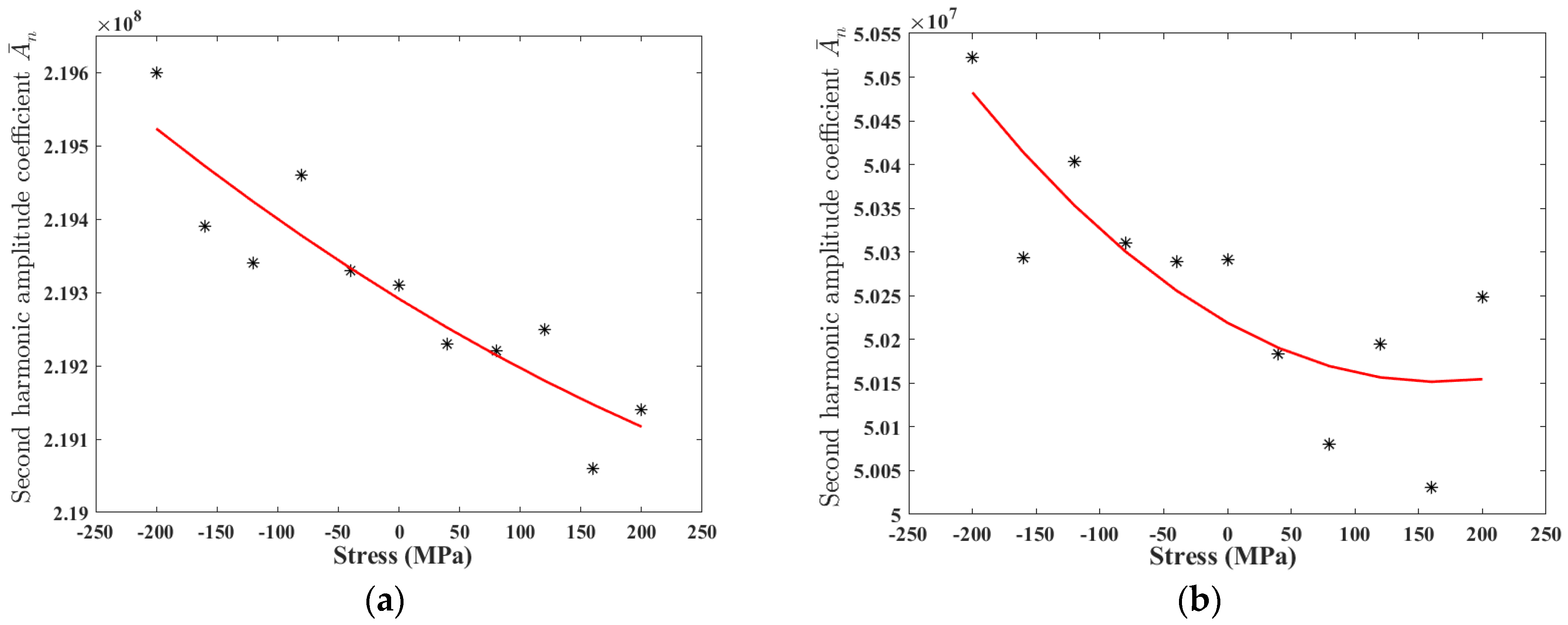
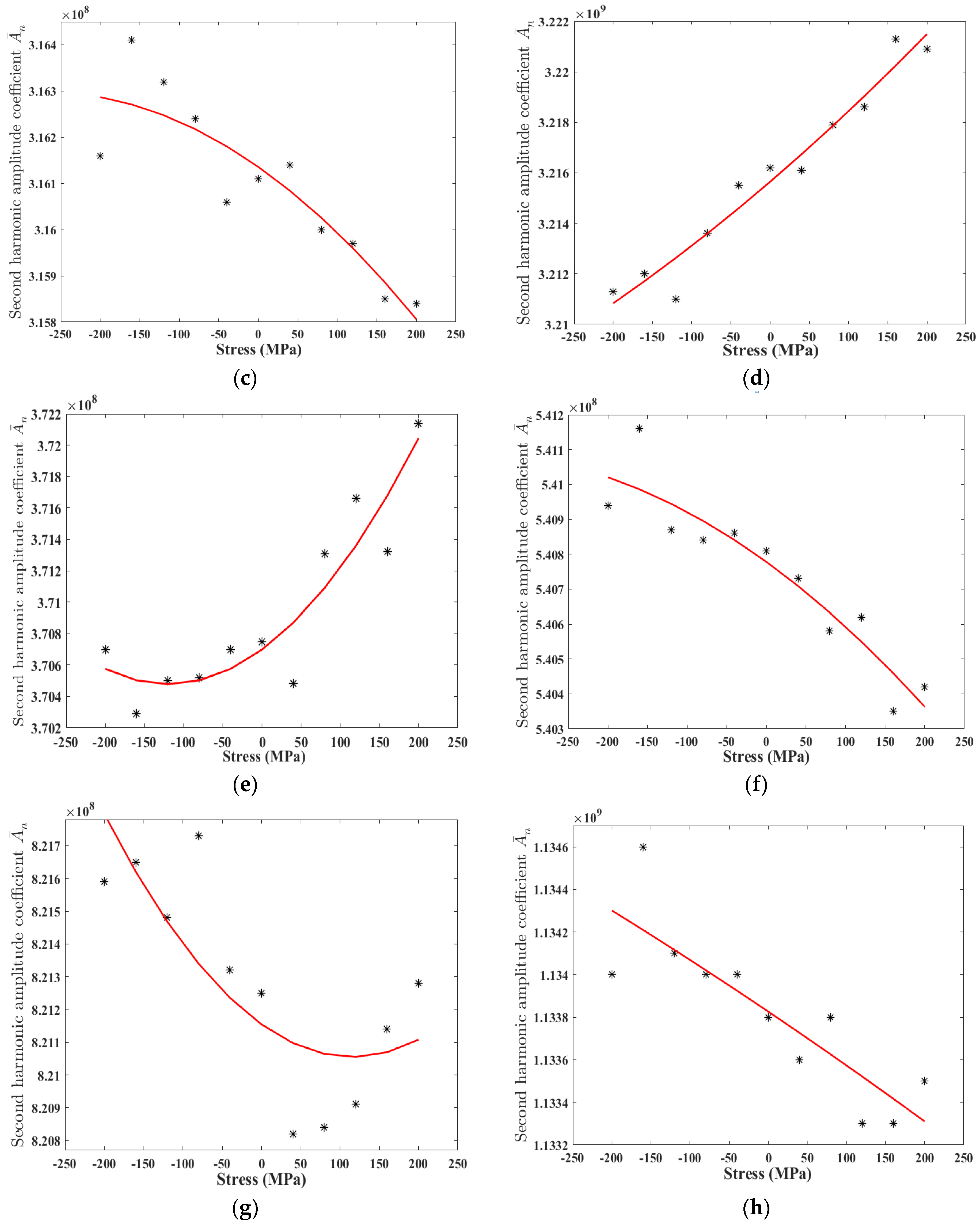
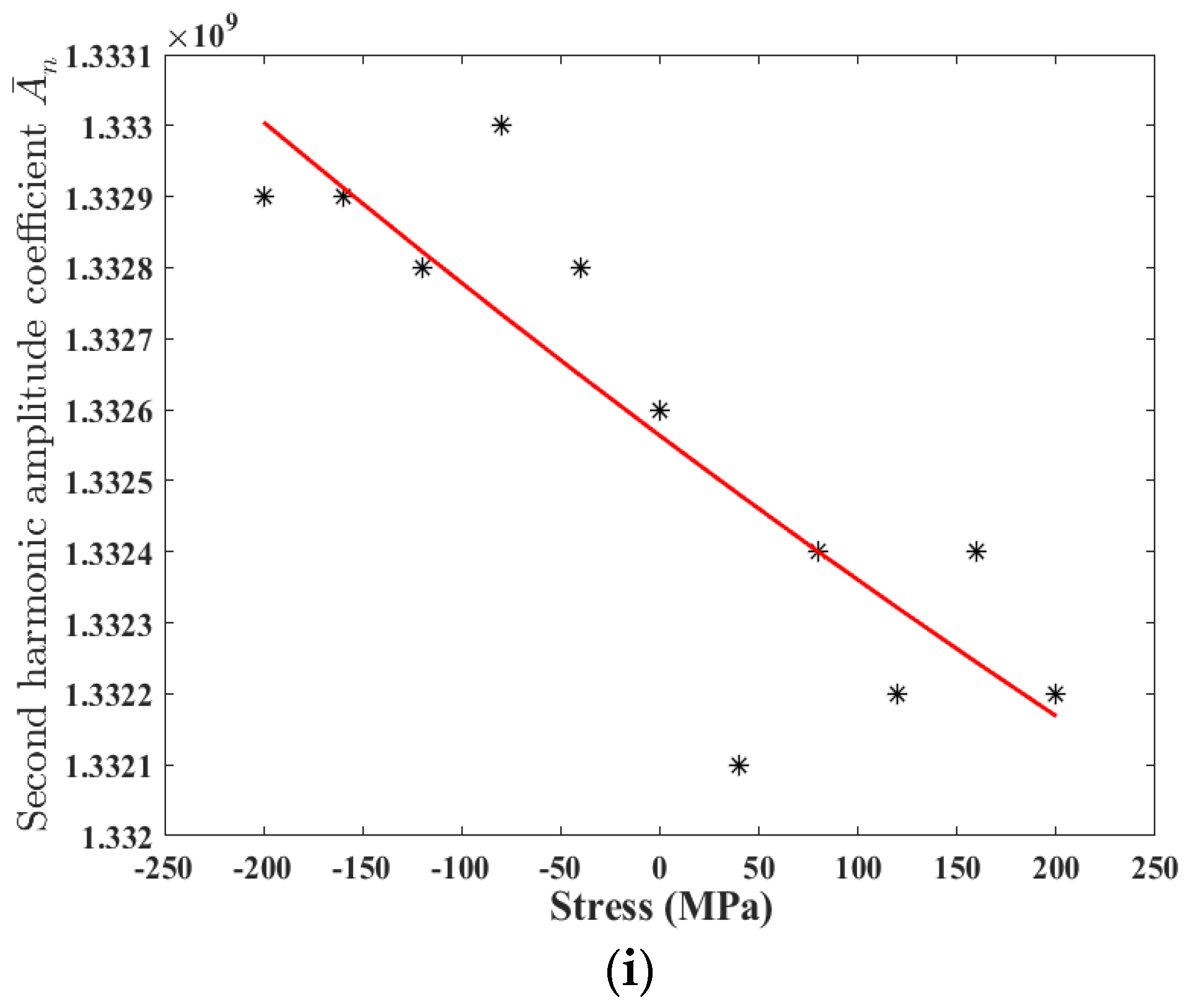
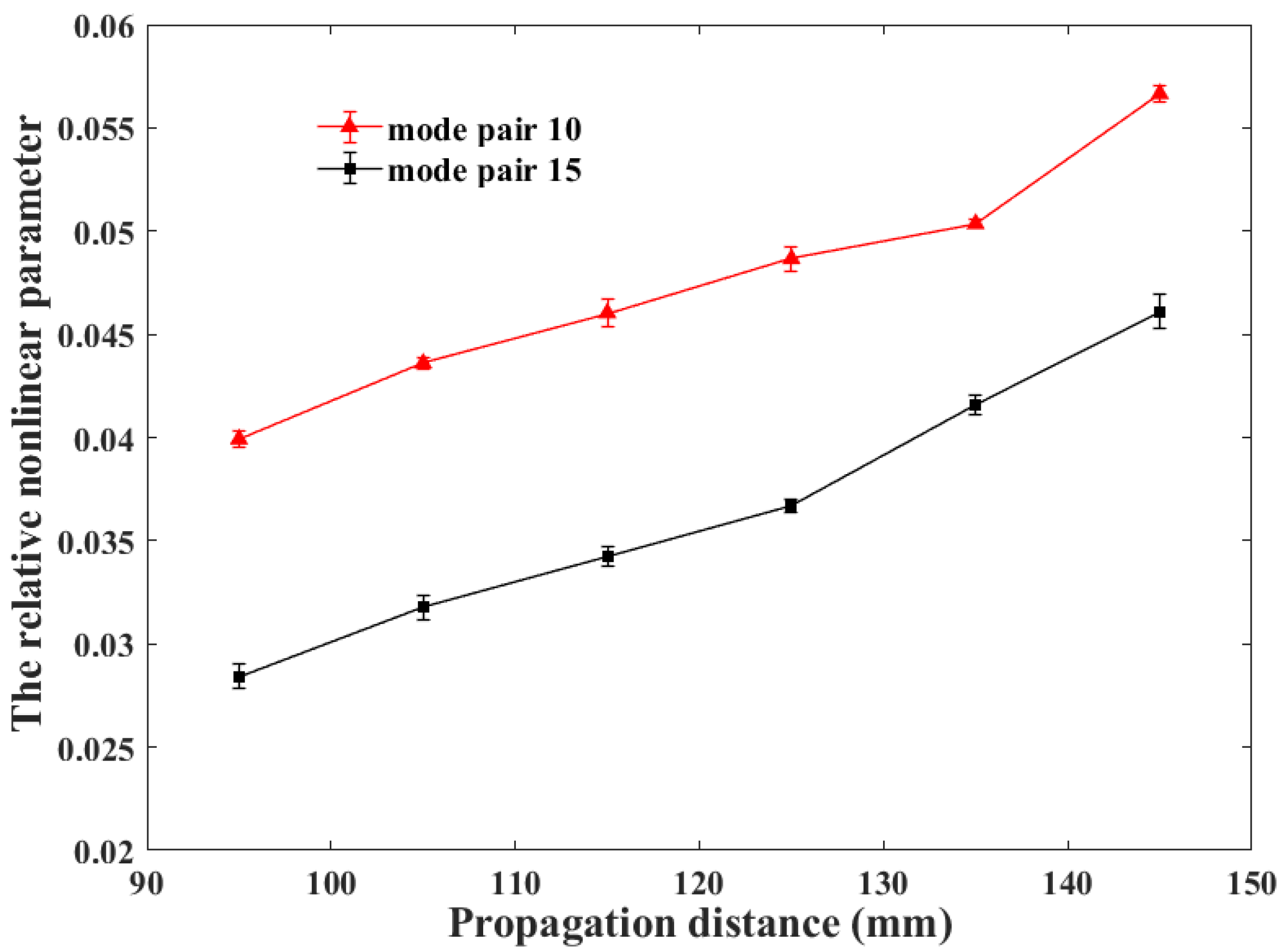
3.3. Response of Second Harmonics under Stress

In this paper, it is assumed that the plate is subjected to axial stress and other directions are in free state. After determining the mode pairs, assume that the axial stress on the steel plate gradually increases from the compressive stress of -200 MPa to the tensile stress of 200 MPa, and the stress changes by 40 MPa each time. By substituting the stress value into Equation (26), the dispersion curves of phase velocity and group velocity of Lamb waves in the steel plate under definite stress are acquired. The mode shapes of the corresponding mode pair can be extracted from the dispersion curves. Substitute the corresponding mode shapes into Equation (18), and the amplitude coefficient ${\overline{A}}_n(x)$ of second harmonic modes generated by this mode pair under definite stress are obtained. After getting the magnitude of the amplitude coefficient, ${\overline{A}}_n(x)$, of the second harmonic mode under different stress, the change trends of ${\overline{A}}_n(x)$ are estimated by using the Least Squares method, as shown in Figure 7.

Figure 7 presents that during the stress change process from -200 MPa compressive stress to 200 MPa tensile stress, the amplitudes of the second harmonic modes generated by mode pairs 7–9 and 12–15 decrease gradually, and the amplitudes of the second harmonic modes generated by mode pairs 10 and 11 increase gradually. In Figure 7, the amplitude coefficient, ${\overline{A}}_n(x)$, shows a monotonic change trend, but the change slope is not always constant, indicating that the change trend of the second harmonic amplitude with the change of stress is not linear. The change of ${\overline{A}}_n(x)$ is mainly due to the change of the mode shapes about the mode pair, and the change of the mode shapes come from the influence of the axial stress on the plate. Therefore, the variation trend of ${\overline{A}}_n(x)$ can be used to express the change of the amplitude of the second harmonic mode with the stress. The simulation results also show that the change trends of the second harmonic modal amplitudes with the stress are not the same when different excitation and reception modes are selected. The method can be applied to provide the anticipation for the variation of the amplitude of second harmonic generated by mode pair in the nonlinear ultrasonic guided waves experiments.

It should be noted that the numerical changes of some data points in Figure 7 are not consistent with the overall change trend. The error data points are caused by the small deviation of the dispersion curve obtained by Equation (26) after the stress is applied, which leads to the inaccuracy of some mode shapes extracted. The small change of mode shapes eventually leads to the appearance of wrong data points. Since the method proposed in this paper is used to predict the change trend of cumulative second harmonic mode in plate under stress, the existence of error points will not affect the overall trend identification. By increasing the number of simulation data points, we make the change trends of cumulative second harmonic modes obtained by this method accurate.

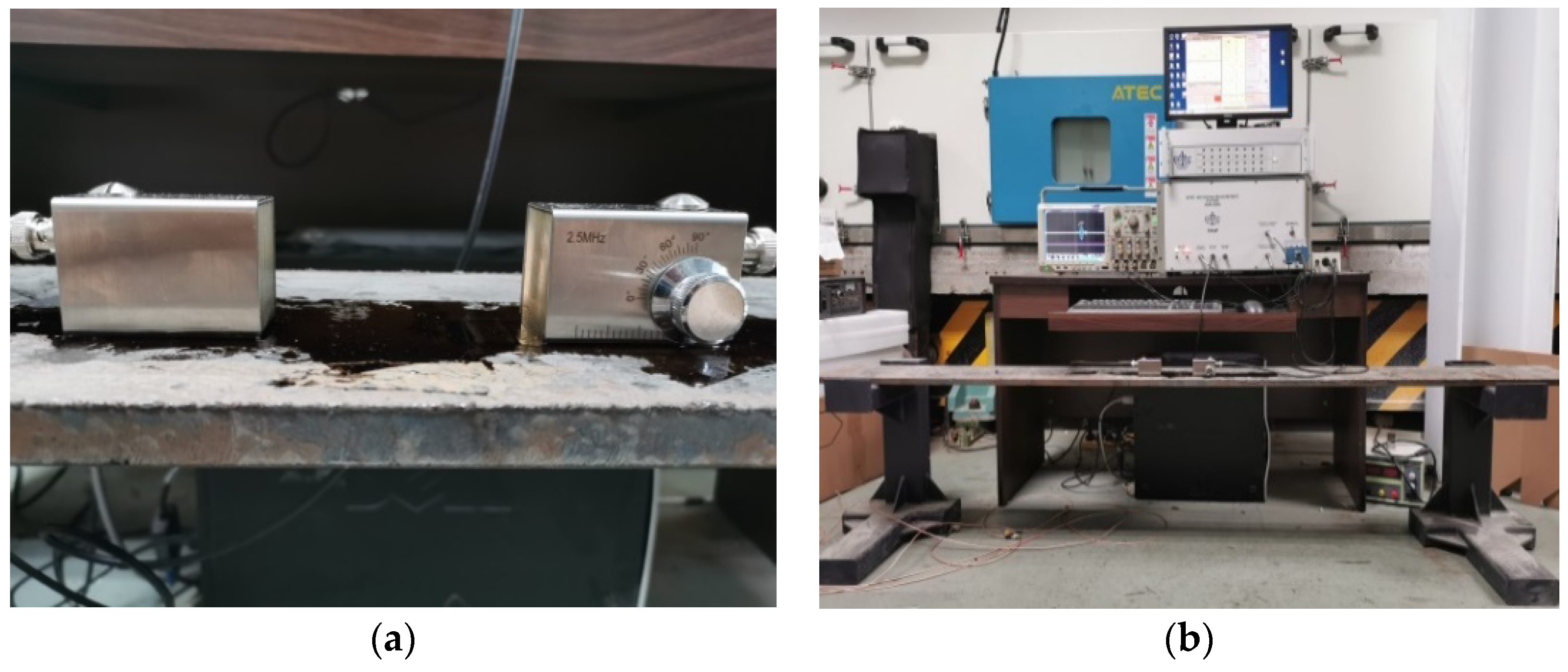
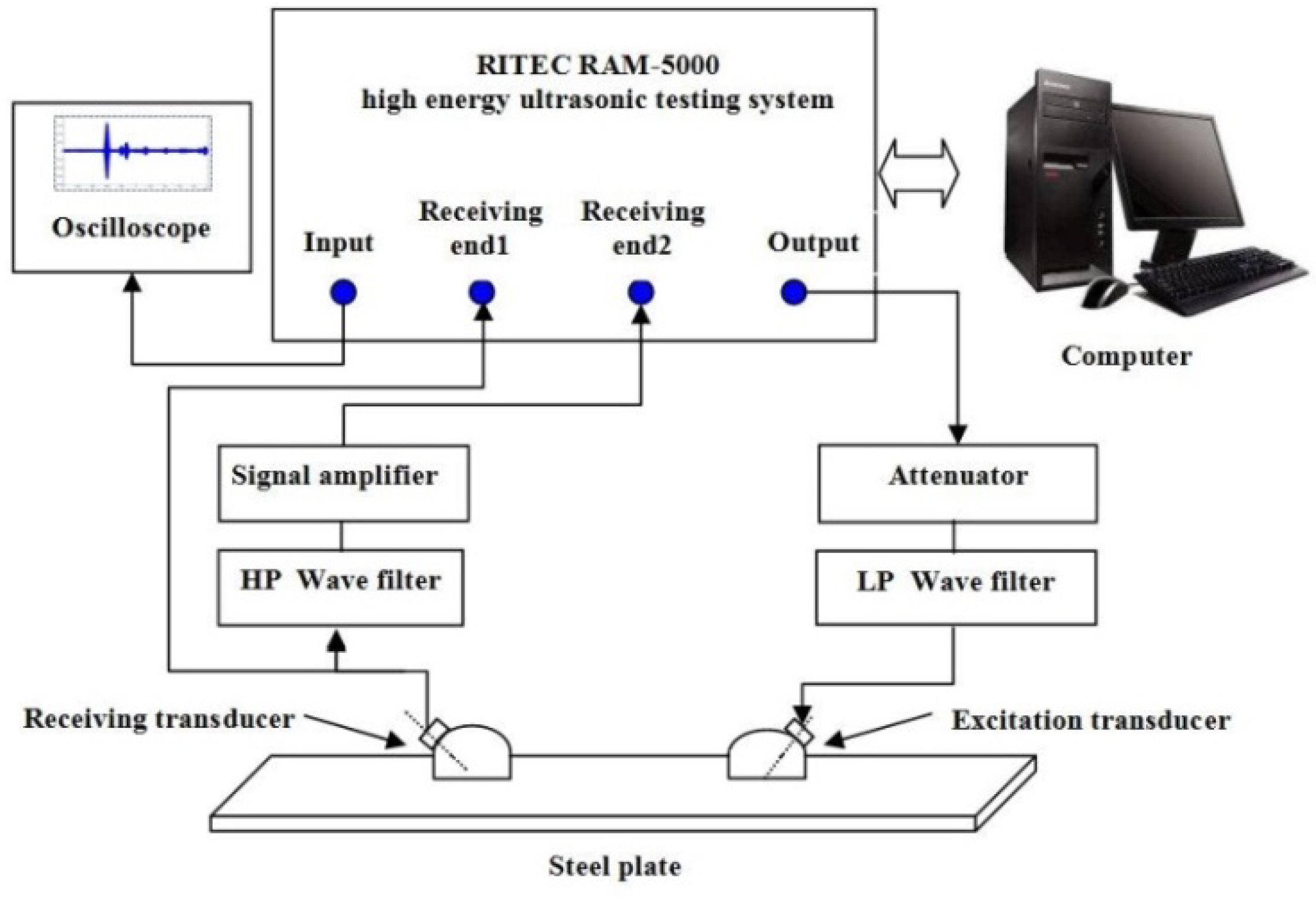
4. Experimental Verifications

The validation experiments are designed for a steel plate with a thickness of 15 mm, length of 2 m, and width of 20 cm. The material properties of the steel plate are listed in Table 1. In order to make a comparison, one mode pair from mode pairs with increasing second harmonic amplitude (mode pair 10 and 11), another mode pair from mode pairs with decreasing second harmonic amplitude (mode pair 7–9, 12–15), and another mode pair from mode pairs with no second harmonic (mode pair 1–6) are selected. It can be seen from Figure 5 that the amplitude coefficients, ${\overline{A}}_n(x)$, of mode pairs 10 and 15 are the largest in the same type of mode pairs, so the amplitudes of the second harmonics generated by mode pairs 10 and 15 are also the largest. Therefore, the mode pairs 6, 10, and 15 in Table 2 are selected as excitation and reception modes, respectively, and the amplitudes of second harmonics of different mode pairs are compared. In the experiment, the longitudinal wave angle probes with adjustable angle are used as the excitation and receiving transducers, and the distance between the excitation transducer and the receiving transducer is 95 mm.

The excitation and receiving angles of transducers meet Snell’s theorem, as follows:

$$\frac{\sin \theta }{C_{\mathrm{glass}}}=\frac{\sin {90}^{\circ }}{C_p}$$

(27)

where $C_{\mathrm{glass}}$ is the speed of ultrasonic waves propagating in plexiglass, $C_{\mathrm{glass}}=2740m/s$. $C_p$ is the phase velocity of ultrasonic waves propagating in steel plate; the $C_p$ corresponding to mode pairs 6, 10, and 15 is $C_{p1}=5904m/s$, $C_{p2}=3933m/s$, and $C_{p3}=3376m/s$, respectively. Substitute the above values into Equation (27) and get ${\theta }_1={28}^{\circ }$, ${\theta }_2={44}^{\circ }$, and ${\theta }_3={55}^{\circ }$. The excitation and receiving transducers are placed on the steel plate, as shown in Figure 8a. In the experiment, the surface of the place where the transducers are placed is flat, which ensures there is no micro crack and bulge. At the same time, a coupling agent with good viscosity is added between the transducer and the steel plate, to increase the bonding strength of the interface and further improve the signal transmission efficiency. The Ritec Ram-5000 high-energy ultrasonic test system is used to excite and receive the signal of the ultrasonic transducers, as shown in Figure 8b. The test system can amplify the maximum excitation signal by 100 times. Because the signal excitation, amplification, and reception are completed by the same test system, the loss of signal strength in the process of transmission is greatly reduced. The experimental system diagram is shown in Figure 9.

In the experiment, the excitation signal is a 20-period sine wave modulated by the Hanning window, with a frequency of 2.5 MHz. At the same excitation amplitude, by adjusting the inclination angle of the transducers, the selection of mode pair is changed. The experimental received signal from mode pair 10 is shown in Figure 10 (the received signals of mode pairs 6 and 15 are similar). Fast Fourier transform (FFT) is performed on the inner part of the circle of the received signal, under each mode pair, to extract the basic frequency and second harmonic signals. The experimental spectrum analysis results are shown in Figure 11.

Figure 11 illustrates that, when mode pairs 10 and 15 are selected as the excitation and reception modes, the received signals have obvious second harmonic, while mode pair 6 is selected as the excitation and reception mode, without obvious second harmonic. Under the same excitation amplitude, the second harmonic amplitude of mode pair 10 is larger than that of mode pair 15. The critical refraction method is used to excite and receive the selected modes that near the phase velocity which satisfies Snell’s theorem. Only the second harmonic generated by the modes pair satisfying the conditions (phase-matching and non-zero power flux) play a dominant role in the field of second harmonic signal [30]. The mode shapes of mode pairs 10 and 15 are shown in Figure 12.

In order to verify that mode pair 10 and 15 can generate cumulative second harmonic, change the dip angle of transducers and gradually increase the distance between the excitation transducer and the receiving transducer from 95 to 145 mm. Calculate and observe the change of the relative nonlinear parameter, $\beta$, according to Equation (23) in the process of distance increase. For every 10 mm increase in the distance, the test system samples 200 times, to calculate the mean value and variance of the relative nonlinear parameter at this distance. The final curve of the relative nonlinear parameter with the distance is shown in Figure 13.

Figure 13 elucidates that with the mode pairs 10 and 15, the relative nonlinear parameters increase gradually with the increase of propagation distance. It denotes that cumulative second harmonics can be generated by using the mode pairs 10 and 15 as the excitation and reception modes. Moreover, under the same propagation distance, the relative nonlinear parameter detected by mode pair 10 is larger than that detected by mode pair 15, which shows that second harmonic mode generated by mode pair 10 has higher amplitude.

To check the changes of second harmonic modal amplitudes generated by the mode pairs 10 and 15 with the change of stress, the steel plate is stressed by the hydraulic tensile machine, which is shown in Figure 14. The distance between the excitation transducer and the receiving transducer is 145 mm, and other experimental settings remain unchanged. The tensile stress of 0 to 25 MPa is applied to the steel plate by the hydraulic tensile machine, with each increase of 5 MPa. The relative nonlinear parameters under different stress conditions are calculated. The experimental results are shown in Figure 15.

Figure 15 shows that the relative nonlinear parameter detected by mode pair 10 increases with the increase of tensile stress, while the relative nonlinear parameter detected by mode pair 15 decreases with the increase of tensile stress. Compared with Figure 7d,i, it can be found that the experimental results are consistent with the simulation results.

5. Conclusions

In this article, a method is advanced to intuitively and effectively determine the response law of the amplitudes of different cumulative second harmonic modes to the stress change in plate by calculating the amplitude coefficient of second harmonic mode under the stress state. The steel plate is further simulated and verified by experiments. The simulation and experimental results confirm the validity of the method and show that when the nonlinear ultrasonic guided waves are applied to detect the stress in plate, the amplitudes of second harmonic modes produced by the different excitation and receiving modes have different trends with the change of stress, which are monotonically decreasing or increasing. The research results also reveal that when choosing the mode pair that can produce cumulative second harmonic mode with the largest amplitude, the value of $f_n{}^{surf}+f_n{}^{vol}$ cannot be taken as the standard completely. It is necessary to calculate and compare the amplitudes of second harmonic modes produced by different mode pairs. It is worth noting that the method proposed in this article relies on the SAFE model of plate to estimate the dispersion curves and mode shapes, and it is applicable to a waveguide with arbitrary cross-section, as long as its dispersion curves and mode shapes can be obtained, e.g., using SAFE method.

References

1. Kawashima, K.; Omote, R.; Ito, T.; Fujita, H.; Shima, T. Nonlinear acoustic response through minute surface cracks: FEM simulation and experimentation. Ultrasonics 2002, 40, 611–615. [Google Scholar] [CrossRef]
2. Brotherhood, C.J.; Drinkwater, B.W.; Dixon, S. The detectability of kissing bonds in adhesive joints using ultrasonic techniques. Ultrasonics 2003, 41, 521–529. [Google Scholar] [CrossRef]
3. Bermes, C.; Kim, J.Y.; Qu, J.; Jacobs, L.J. Experimental characterization of material nonlinearity using Lamb waves. Appl. Phys. Lett. 2007, 90, 2067–2073. [Google Scholar] [CrossRef]
4. Walker, S.V.; Kim, J.Y.; Qu, J.; Jacobs, L.J. Fatigue damage evaluation in A36 steel using nonlinear Rayleigh surface waves. NDT&E Int. 2012, 48, 10–15. [Google Scholar]
5. Kim, G.; In, C.W.; Kim, J.Y.; Kurtis, K.E.; Jacobs, L.J. Air-coupled detection of nonlinear Rayleigh surface waves in concrete-application to microcracking detection. NDT&E Int. 2014, 67, 64–70. [Google Scholar]
6. Thiele, S.; Kim, J.Y.; Qu, J.; Jacobs, L.J. Air-coupled detection of nonlinear Rayleigh surface waves to assess material nonlinearity. Ultrasonics 2014, 54, 1470–1475. [Google Scholar] [CrossRef]
7. Xiang, Y.X.; Deng, M.X.; Xuan, F.Z. Creep damage characterization using nonlinear ultrasonic guided wave method: A mesoscale model. J. Appl. Phys. 2014, 115, 044914. [Google Scholar] [CrossRef]
8. Rose, J.L.; Avioli, M.J.; Mudgec, P.; Sanderson, R. Guided wave inspection potential of defects in rail. NDT&E Int. 2004, 37, 153–161. [Google Scholar]
9. Mazzotti, M.; Marzani, A.; Bartoli, I.; Viola, E. Guided waves dispersion analysis for prestressed viscoelastic waveguides by means of the SAFE method. Int. J. Solids Struct. 2012, 49, 2359–2372. [Google Scholar] [CrossRef] [Green Version]
10. Xing, B.; Yu, Z.J.; Xu, X.N.; Zhu, L.Q.; Shi, H.M. Research on a Rail Defect Location Method Based on a Single Mode Extraction Algorithm. Appl. Sci. 2019, 9, 1107. [Google Scholar] [CrossRef] [Green Version]
11. Xu, X.N.; Xing, B.; Zhuang, L.; Shi, H.M.; Zhu, L.Q. A Graphical Analysis Method of Guided Wave Modes in Rails. Appl. Sci. 2019, 9, 1529. [Google Scholar] [CrossRef] [Green Version]
12. Shi, H.M.; Zhuang, L.; Xu, X.N.; Yu, Z.J.; Zhu, L.Q. An Ultrasonic Guided Wave Mode Selection and Excitation Method in Rail Defect Detection. Appl. Sci. 2019, 9, 1170. [Google Scholar] [CrossRef] [Green Version]
13. Duan, X.Y.; Zhu, L.Q.; Yu, Z.J.; Xu, X.N. Estimating the Axial Load of In Service Continuously Welded Rail Under the Influences of Rail Wear and Temperature. IEEE Access 2019, 7, 143524–143538. [Google Scholar] [CrossRef]
14. Bartoli, I.; Nucera, C.; Srivastava, A.; Salamone, S.; Phillips, R.; Di Scalea, F.; Coccia, S.; Sikorsky, C.S. Nonlinear ultrasonic guided waves for stress monitoring in prestressing tendons for post-tensioned concrete structures. Proc. SPIE 2009, 19, 230–235. [Google Scholar]
15. Bartoli, I.; Coccia, S.; Phillips, R.; Srivastava, A.; Di Scalea, F.; Salamone, S. Stress dependence of guided waves in rails. Proc. SPIE 2010, 7650, 2101–2110. [Google Scholar]
16. Liu, M.; Kim, J.Y.; Qu, J.; Jacobs, L.J. Measuring residual stress using nonlinear ultrasound. API Conf. Proc. 2010, 1211, 1365–1372. [Google Scholar]
17. Liu, M.; Kim, J.Y.; Jacobs, L.J.; Qu, J. Experimental study of nonlinear Rayleigh wave propagation in shot-peend aluminum plates—Feasibility of measuring residual stress. NDT&E Int. 2011, 44, 67–74. [Google Scholar]
18. Yan, H.J.; Xu, C.G.; Xiao, D.G.; Cai, H.C. Research on Nonlinear Ultrasonic Properties of Tension Stess in Metal Materials. J. Mec. Eng. 2016, 52, 22–29. [Google Scholar] [CrossRef]
19. Yan, H.J.; Liu, F.B.; Pan, Q.X. Nonlinear Ultrasonic Properties of Stress in 2024 Aluminum. Adv. Mat. Res. 2017, 1142, 371–377. [Google Scholar] [CrossRef]
20. Auld, B.A. Acoustic Fields and Waves in Solids; Robert E. Krieger Publishing Company: Malabar, FL, USA, 1990. [Google Scholar]
21. Deng, M.X. Cumulative second-harmonic generation accompanying nonlinear shear horizontal mode propagation in a solid plate. J. Appl. Phys. 1998, 84, 3500–3505. [Google Scholar]
22. Deng, M.X. Cumulative second-harmonic generation of Lamb-modes propagation in a solid plate. J. Appl. Phys. 1999, 85, 3051–3058. [Google Scholar] [CrossRef]
23. Deng, M.X. Analysis of second-harmonic generation of Lamb modes using a modal analysis approach. J. Appl. Phys. 2003, 94, 4152–4159. [Google Scholar] [CrossRef]
24. De Lima, W.J.N.; Hamilton, M.F. Finite-amplitude waves in isotropic elastic plates. J. Sound Vib. 2003, 265, 819–839. [Google Scholar] [CrossRef]
25. De Lima, W.J.N.; Hamilton, M.F. Finite amplitude waves in isotropic elastic waveguides with arbitrary constant cross sectional area. Wave Motion 2005, 41, 1–11. [Google Scholar] [CrossRef]
26. Chillara, V.K.; Lissenden, C.J. Interaction of guided wave modes in isotropic weakly nonlinear elastic plates: Higher harmonic generation. J. Appl. Phys. 2012, 111, 4909–4915. [Google Scholar]
27. Srivastava, A.; Di Scalea, F. On the existence of antisymmetric or symmetric Lamb waves at nonlinear higher harmonics. J. Sound Vib. 2009, 323, 932–943. [Google Scholar] [CrossRef]
28. Lee, T.H.; Choi, I.H. The nonlinearity of guided wave in an elastic plate. Mod. Phys. Lett. B 2008, 22, 1135–1140. [Google Scholar] [CrossRef]
29. Pruell, C.; Kim, J.Y.; Qu, J.; Jacobs, L.J. Evaluation of plasticity driven material damage using Lamb waves. Appl. Phys. Lett. 2007, 91, 231911. [Google Scholar] [CrossRef]
30. Deng, M.X.; Xiang, Y.; Liu, L. Time-domain analysis and experimental examination of cumulative second-harmonic generation by primary Lamb wave propagation. J. Appl. Phys. 2011, 109, 113525. [Google Scholar] [CrossRef] [Green Version]
31. Liu, Y.; Kim, J.Y.; Jacobs, L.J.; Qu, J.; Li, Z. Experimental investigation of symmetry properties of second harmonic Lamb waves. J. Appl. Phys. 2012, 111, 381–389. [Google Scholar] [CrossRef]
32. Liu, Y.; Chillara, V.K.; Lissenden, C.J. On selection of primary modes for generation of strong internally resonant second harmonics in plates. J. Sound Vib. 2013, 33, 4517–4528. [Google Scholar] [CrossRef]
33. Landau, L.D.; Lifshitz, E.M. Theory of Elasticity, 2nd ed.; Permagon Press: New York, NY, USA, 1970. [Google Scholar]
34. Chillara, V.K.; Lissenden, C.J. Nonlinear guided waves in plates: A numerical perspective. Ultrasonics 2014, 54, 1553–1558. [Google Scholar] [CrossRef] [PubMed]
35. Goldberg, Z.A. Interaction of plane longitudinal and transverse elastic waves. Sov. Phys. Acoust. 1960, 6, 306–310. [Google Scholar]
36. Nucera, C.; Di Scalea, F. Nonlinear Semianalytical Finite-Element Algorithm for the Analysis of Internal Resonance Conditions in Complex Waveguides. J. Eng. Mech. 2014, 140, 502–522. [Google Scholar] [CrossRef]
37. Müller, M.F.; Kim, J.Y.; Qu, J.; Jacobs, L.J. Characteristics of second harmonic generation of Lamb waves in nonlinear elastic plates. J. Acoust. Soc. Am. 2010, 127, 2141–2152. [Google Scholar] [CrossRef] [PubMed] [Green Version]
38. Loveday, P.W. Semi-analytical finite element analysis of elastic waveguides subjected to axial loads. Ultrasonics 2008, 49, 298–300. [Google Scholar] [CrossRef]
39. Nucera, C.; Di Scalea, F. Nondestructive measurement of neutral temperature in continuous welded rails by nonlinear ultrasonic guided waves. J. Acoust. Soc. Am. 2014, 136, 2561–2574. [Google Scholar] [CrossRef]
Figure 1. Semi-analytical finite element (SAFE) model of wave propagating in plate.
Applsci 10 05124 g001
Figure 2. Discretization of a plate with one-dimensional three-node elements.
Applsci 10 05124 g002
Figure 3. Phase velocity dispersion curves of isotropic steel plate.
Applsci 10 05124 g003
Figure 4. Group velocity dispersion curves of isotropic steel plate.
Applsci 10 05124 g004
Figure 5. Amplitude coefficients of cumulative second harmonic modes vary according to propagation distance.
Applsci 10 05124 g005
Figure 6. Amplitude coefficients of non-cumulative second harmonic modes vary according to propagation distance.
Applsci 10 05124 g006
Figure 7. Amplitudes of the second harmonic mode generated by mode combinations vary with the stress: (a) mode pair 7; (b) mode pair 8; (c) mode pair 9; (d) mode pair 10; (e) mode pair 11; (f) mode pair 12; (g) mode pair 13; (h) mode pair 14; and (i) mode pair 15.
Applsci 10 05124 g007aApplsci 10 05124 g007bApplsci 10 05124 g007c
Figure 8. Physical experiment system: (a) the excitation and receiving angle probes for Lamb waves in the steel plate; (b) high-energy ultrasonic testing system.
Applsci 10 05124 g008
Figure 9. The experimental system’s diagram.
Applsci 10 05124 g009
Figure 10. Signal diagram.
Applsci 10 05124 g010
Figure 11. Spectrum analysis diagram.
Applsci 10 05124 g011
Figure 12. The mode shapes of mode 10 and 15: (a) the fundamental mode of mode pair 10; (b) the second harmonic mode of mode pair 10; (c) the fundamental mode of mode pair 15; and (d) the second harmonic mode of mode pair 15.
Applsci 10 05124 g012aApplsci 10 05124 g012b
Figure 13. Nonlinear parameter versus propagation distances.
Applsci 10 05124 g013
Figure 14. Steel plate tensile test system.
Applsci 10 05124 g014
Figure 15. Experimental results of nonlinear parameter change with stress.
Applsci 10 05124 g015