Article

A Multi-Level Non-Uniform Spatial Sampling Method for Accuracy Assessment of Remote Sensing Image Classification Results

College of Information Science, Shanghai Ocean University, Shanghai 201306, China
*
Authors to whom correspondence should be addressed.
Appl. Sci. 2020, 10(16), 5568; https://doi.org/10.3390/app10165568
Submission received: 17 June 2020 / Revised: 1 August 2020 / Accepted: 5 August 2020 / Published: 11 August 2020

Abstract

:
Accuracy assessment of classification results has important significance for the application of remote sensing images, which can be achieved by sampling methods. However, the existing sampling methods either ignore spatial correlation or do not consider spatial heterogeneity. Here, we proposed a multi-level non-uniform spatial sampling method (MNSS) for the accuracy assessment of classification results. Taking the remote sensing image of Kobo Askov, Texas, USA, as an example, the classification result of this image was obtained by Support Vector Machine (SVM) classifier. In the proposed MNSS, the studied spatial region was zoned from high to low resolution based on the features of spatial correlation. Then, the sampling rate of each zone was deduced from the low to high resolution based on the spatial heterogeneity. Finally, the positions of sample points were allocated in each zone, and the classification results of the sample points were obtained. We also used other sampling methods, including a random sampling method (SRS), stratified sampling method (SS), and spatial sampling of the gray level co-occurrence matrix method (GLCM), to obtain the classification results of the sample points (2-m resolution). Five categories of ground objects in the same region were used as the ground truth data. We than calculated the overall accuracy, Kappa coefficient, producer accuracy, and user accuracy to estimate the accuracy of the classification results. The results showed that MNSS was the strictest inspection method as shown by the minimum value of accuracy. Moreover, MNSS overcame the shortcoming of SRS, which did not consider the spatial correlation of sample points, and overcame the shortcomings of SS and GLCM, which had redundant information between sample points. This paper proposes a novel sampling method for the accuracy assessment of classification results of remote sensing images.

1. Introduction

Remote sensing images have been widely used in many aspects of earth observation. Most notably, the classification of remote sensing image is a key step for the application of remote sensing images [1]. Accuracy assessment is a fundamental component of classification analysis [2]. Accuracy assessment is required to be conducted before the application of classification results of remote sensing for scientific investigation and policy decision [3].
The sampling method is an effective tool for performing accuracy assessment [4,5]. Traditional sampling methods, including simple random sampling method [6], stratified sampling method [7], systematic sampling method [8], and cluster sampling method [9], have been used for the accuracy assessment of classification results of remote sensing images. Koyuncu et al. proposed a new calibration estimator to estimate the population mean in stratified random sampling [10]. Using stratified sampling method, Wickham et al. reported agreement statistics between map and reference labels for national land cover database (NLCD) 2011, which includes land cover for ca. 2001, ca. 2006, and ca. 2011 [4]. Di et al. developed a reasonable spatial sampling plan for crop area estimation based on the SPOT-5 image, combined with the selection of stratified standards and the size of sampling units [11]. However, these sampling methods are more suitable for the accuracy assessment of products with independent items. By contrast, remote sensing images have dependent feature information and are characterized by spatial correlation and spatial heterogeneity. Recently, several sampling methods were proposed for the accuracy assessment of spatial images. Meng et al. used the spatial stratified sampling method for the accuracy assessment of regional surface coverage [12]. Wang et al. proposed a “sandwich” sampling model for the accuracy assessment of small-cultivated land areas [13]. Stehman proposed a unified framework for crop area estimation based on a confusion matrix [14]. Mayaux et al. calculated the species richness and uniformity of each sample grid using a diversity index (Shannon–Weaver (SW)) [15]. These spatial sampling methods only consider the feature of spatial correlation and ignore spatial heterogeneity. Spatial heterogeneity is also an important determinant in accuracy assessment. Spatial heterogeneity within pixels biases the non-linear estimation of classification variables from remote sensing images.
In this study, a multi-level non-uniform spatial sampling method (MNSS) was proposed for the accuracy assessment of classification results of remote sensing images, which was deduced by calculating spatial correlation and heterogeneity.

2. Methodology

Here, the remote sensing images were classified using the SVM classifier. The kernel function of SVM is the radial basis function (RBF), defined by [16]
k ( x , z ) = exp ( - d ( x , z ) 2 2 × σ 2 ) = exp ( - g a m m a d ( x , z ) 2 ) g a m m a = 1 2 . σ 2
where d ( x , z ) is the Euclidean distance from point x to the center of kernel function z . σ is the width parameter, which controls the radial action range. Gamma is a parameter of the RBF function after it is selected as a kernel. The larger the gamma, and the less the support vector, while the smaller the gamma value, the more support vectors. C is the penalty coefficient, namely, the tolerance of error. The higher the C value, the greater the amount of error that cannot be tolerated, and overfitting is easy.
Figure 1 shows the flow chart of the accuracy assessment of the classification results of remote sensing images.
The proposed MNSS consists of three steps. In step 1, the fragmentation indexes of the classification results are calculated based on spatial autocorrelation, and then the studied region is zoned from high to low resolution based on the fragmentation indexes. In step 2, the sampling rate for each zone is deduced from the low to high resolution based on spatial heterogeneity. In step 3, the position of each sample point is selected, and the accuracy of the classification results is accessed by comparing each sample point with the ground truth data.

2.1. Step 1: The Studied Region was Zoned from High to Low Resolution

Taking the classification results of remote sensing images as the input data, the studied region was zoned by calculating the fragmentation index (F), as shown in Figure 2.
The fragmentation index (F) indicates the fragmentation degree of the study region, reflecting the spatial complexity of the region [17].
F is calculated as
F i = A i N i
where Fi is the fragmentation index of the i-th window. Ai is the number of different types of land cover in the i-th window. N is the number of pixels in the i-th window. Here, F was calculated by a 3 × 3 pixel window. According to F, the regions were zoned from high to low resolution.

2.2. Step 2: The Sampling Rate was Deduced from Low to High Resolution

The sampling rate of each zone was deduced from low to high resolution by Equation (3).
w i t = F i t t = 1 m F i t n i t = n i + 1 × w i t
where i (i = 0, 1, 2, ...) indicates the different spatial scale of the classification results. i = 0 represents the original spatial resolution. F i t is the fragmentation index of the t-zone at the i-th spatial scale, t = 1, 2, ... m. m is the zone number at the i-th spatial scale. w i t is the sampling weight coefficient of the t -zone at the i-th spatial scale, i.e., the sampling rate of the t -zone at the i-th spatial scale. n i t is the sample size of the t -zone at the i-th spatial scale.

2.3. Step 3: Accuracy Assessment of the Classification Results

The accuracy of classification results was accessed by comparing each sample point with the ground truth data. In this study, the sample unit of accuracy assessment was the pixel of remote sensing images. The sample size was calculated following [18,19]
n ^ = μ 2 1 α 2 ( 1 p 0 ) r 2 p 0 1 + 1 N ( μ 2 1 α 2 ( 1 p 0 ) r 2 p 0 1 )
where N is the lot size of the pixels of remote sensing images. p is the proportion of nonconforming items, and it denotes the average pixel classification error rate of the remote sensing classifications. p0 is the proportion of the nonconforming estimator, which is the maximum limit of the proportion of nonconforming items allowed in the application of remote sensing classification. r is the maximum relative error between the percent non-conforming estimator p0 and the true value p. μ 1 α / 2 is the critical value of the standard normal distribution at the confidence level 1 α / 2 .
Taking five categories of ground objects in the same region (2-m resolution) as the ground truth data, the accuracy of the classification results was accessed by comparing each sample point with the ground truth data. The sample points were selected in the same regions as the ground truth data (2-m resolution). If the type of land-cover from the two different images was consistent, the variable was assigned a value of 1; otherwise, the variable was assigned a value of 0 [20].

3. Experiment

3.1. Experimental Data

The study region is located in Kobo Askov, Texas, USA. The experiment dataset is the fusion image of multispectral and panchromatic images based on HYDICE (Hyperspectral Digital Imagery Collection Experiment) obtained on April 16, 2015, with 2-m spatial resolution (Figure 3a). The ground truth data were obtained by a structured sparse regularization non-negative matrix decomposition (SS-NMF) method [21], which includes five categories of ground objects in the same region. Both the experimental data and the ground truth data are available at http://www.escience.cn. All datasets follow the same coordinate system, WGS_1984_UTM_zone_50N.
Five different types of land cover were classified, i.e., road, grass, forest, roof, and others based on the SVM in Environment for Visualizing Images (ENVI) 5.1 software (ENVI, a complete remote sensing image processing platform, is the flagship product of Exelis Visual Information Solutions, Boulder, CO, USA.).The classification results are shown in Figure 4.
Here, the lot size of the pixels of the remote sensing image was 94249. Given the accuracy requirement, p0 was 85%, μ 1 α / 2 was 0.80, and r was 1%, according to Equation (4), and the sample size was 1800.

3.2. Performance of the Proposed MNSS

Figure 5 shows the zone results of remote sensing classification at five different spatial scales, from 2-m resolution, 6-m resolution, 18-m resolution, 54-m resolution, to 162-m resolution. According to the zone results, the sampling rate of each zone was deduced from low to high resolution, which was from 162-m resolution, 54-m resolution, 18-m resolution, 6-m resolution, to 2-m resolution. At the fifth level of the spatial resolution, the sampling rate of each zone was determined by the area of each zone to the total studied region area. According to the sampling rate at the fifth level spatial resolution, the sampling rate of each zone was calculated by Equation (2) from low to high resolution. Table 1, Table 2, Table 3, Table 4 and Table 5 show the sampling rate of each zone at different spatial scales.
The sample pixel number of the studied remote sensing image (n) was 1800. According to the sampling rate as shown in Table 5, the sampling size of each zone at the original spatial resolution was determined. And form 1-zone to 5-zone, the sampling size was and it was 355, 459, 378, 456, and 152, respectively.

3.3. Comparison of Accuracy Assessment Efficiency between Different Sampling Methods

In this section, we used four different sampling methods to a conduct accuracy assessment of the classification results, i.e., the simple random sampling method (SRS), stratified sampling method (SS), spatial sampling of the gray level co-occurrence matrix method (GLCM) [2], and our proposed method (MNSS). In order to verify the efficiency of our proposed MNSS, a full inspection was performed. Four indexes were used to evaluate the efficiency of different sampling methods: overall classification accuracy (OA), Kappa coefficient (Kappa), producer accuracy (PA), and user accuracy (UA).
Overall classification accuracy (OA) [22] is the proportion of the correct classification of all categories relative to the total number of samples, reflecting the overall correctness of the classification results [23,24]. The formula is:
O A = i = 1 n m i i j = 1 n i = 1 n m i j
The Kappa coefficient is different from the overall classification accuracy which only uses the diagonal elements of the confusion matrix; it utilizes the entire confusion matrix information and is a comprehensive measure of the classification accuracy [25]. The formula is:
K a p p a = N i = 1 n m i j i = 1 n ( m i + m + i ) N 2 i = 1 n ( m i + m + i )
Producer accuracy (PA) is the ratio of the classifier correctly dividing the cells of the entire image into the number of cells in the class A (diagonal value) and the total number of real references in class A (the sum of the class A columns in the confusion matrix). The formula is:
P A = m i i m + i
User accuracy (UA) is the ratio of the total number of cells (diagonal value) correctly classified into class A and the classifier dividing the cells of the entire image into the total number of cells of class A (the sum of class A rows in the confusion matrix). The formula is:
U A = m i i m i +
where m i + and m + i represent the sum of the rows and columns of the confusion matrix and N is the sum of all items in the confusion matrix.
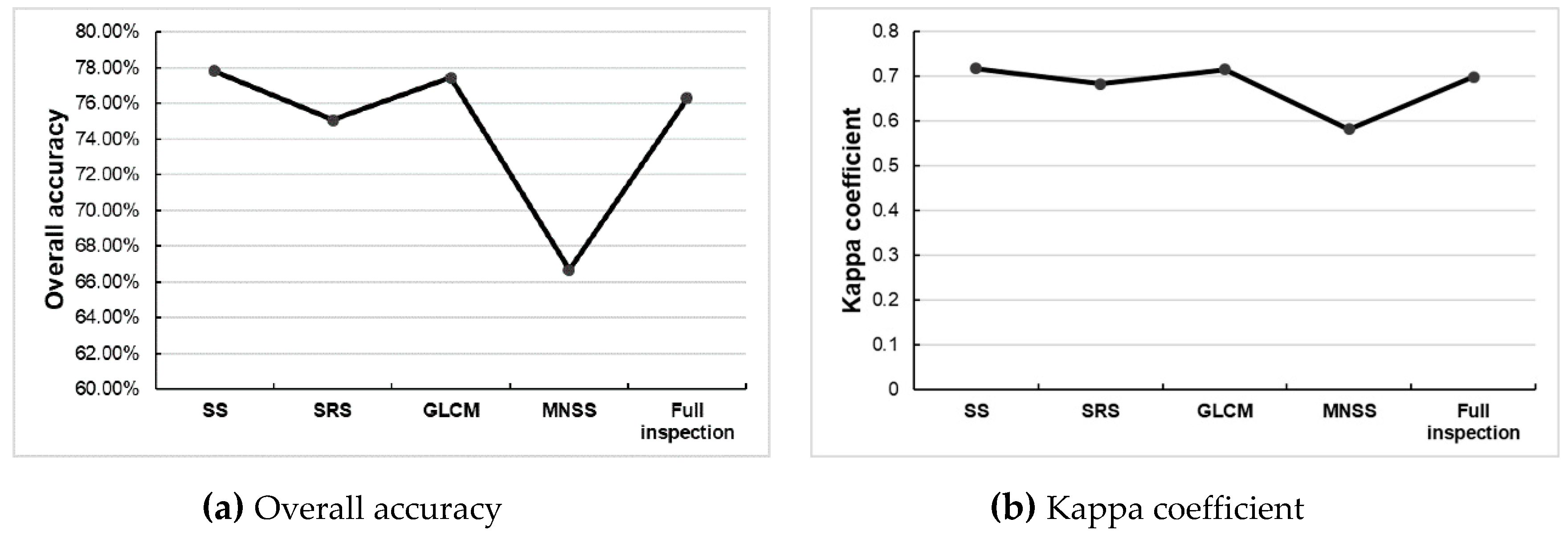
Figure 6 shows the sample points allocated in the studied region by different sampling methods. Table 6 shows the accuracy inspection confusion matrix of the full inspection based on SVM [26]. Figure 7 shows the accuracy assessment by different sampling methods. Figure 8 shows the comparison of producer accuracy (PA) and user accuracy (UA) for different sampling methods.
As shown in Figure 6, compared with random sampling method (SRS), the proposed method overcame the shortcomings that the sample points were randomly distributed in the studied region. Compared with stratified sampling method (SS) and spatial sampling of the gray level co-occurrence matrix method (GLCM), the proposed MNSS reduced the redundant information between different sample points.
From Figure 7 and Figure 8, we can conclude that the accuracy results of our proposed MNSS were lower than those of other methods. By the proposed method, the sample points were located in the region, which had more mixed pixels and was the change boundary of land covers, and also had a higher probability of classification error. The result showed that our proposed MNSS was stricter than other methods and was more suitable for higher accuracy requirements of remote sensing image applications.

4. Discussion

Accuracy assessment of the classification results of remote sensing images is a key step before application for scientific investigation and policy decision. According to the sampling procedures for accuracy assessment by attributes, such as ISO 2859, ISO 19113, or ISO19114, there are three different classes of the accuracy inspection procedures, i.e., reduced inspection, standard inspection, and tightened inspection [27,28,29]. In this study, we designed an accuracy assessment method for the tightened inspection of accuracy assessment of remote sensing image classification results. The tightened inspection of accuracy assessment presented a lower error tolerance rate for the classification results of remote sensing images and was more suitable for higher accuracy requirements of remote sensing image applications.
Our proposed method considered both spatial autocorrelation and spatial heterogeneity during the accuracy assessment. Compared with the existing sampling methods, the proposed method obtained more sample points in the studied region with higher land use fragmentation. The proposed method overcame the shortcomings of the random sampling method (SRS) to avoid sample points randomly allocated in the studied region. Compared with stratified sampling method (SS) and spatial sampling of the gray level co-occurrence matrix method (GLCM), the proposed method significantly reduced the redundant information between different sample points. Thus, our proposed method is more suitable for the accuracy assessment of classification results of remote sensing images.
However, there are some limitations of our proposed method. Our method only considers how to distribute sample points and ignores how to determine the required sample size. In addition, our proposed method only selects a 3 pixel by 3 pixel window for the studied zone. However, we did consider the potential impact of window size on the accuracy assessment of the classification results of remote sensing images.

5. Conclusions

In this study, we proposed a multi-level non-uniform spatial sampling method for the classification results of remote sensing. This method zoned the studied region from high to low spatial resolution, deduced the sampling rate of each zone from low to high resolution, and allocated the sample points to the original spatial resolution. The proposed method ensured that the higher the fragment index of the zoned region, the higher the probability of the sample points allocated in the studied region. Thus, our proposed method is a suitable method for the accuracy assessment of the classification results of remote sensing images.

Author Contributions

Conceptualization, Z.W. and L.W.; Methodology, Z.W. and Q.J.; Validation, W.S. and L.W.; Formal Analysis, Z.W. and W.S.; Investigation, L.X. and Q.J.; Writing-Original Draft Preparation, L.X. and Q.J.; Writing-Review & Editing, Z.W. and L.X.; Supervision, Z.W. and L.W.; Funding Acquisition, Z.W. All authors have read and agreed to the published version of the manuscript.

Funding

This work was generously supported by the grants from the Capacity Development for Local College Project (Grant No. 19050502100 to W.Z.H.).

Acknowledgments

We would like to thank the anonymous reviewers for their valuable suggestions.

Conflicts of Interest

The authors declare no conflict of interest.

References

  1. Stehman, S.V.; Czaplewski, R.L. Design and analysis for thematic map accuracy assessment: Fundamental principles. Remote Sens. Environ. 1998, 64, 331–344. [Google Scholar] [CrossRef]
  2. Huang, D.; Xu, S.; Sun, J.; Liang, S.; Song, W.; Wang, Z. Accuracy assessment model for classification result of remote sensing image based on spatial sampling. J. Appl. Remote Sens. 2017, 11, 046023. [Google Scholar] [CrossRef] [Green Version]
  3. Foody, G.M. Latent Class Modeling for Site- and Non-Site-Specific Classification Accuracy Assessment Without Ground Data. IEEE Trans. Geosci. Remote Sens. 2012, 50, 2827–2838. [Google Scholar] [CrossRef]
  4. Wickham, J.; Stehman, S.V.; Gass, L.; Dewitz, J.A.; Sorenson, D.G.; Granneman, B.J.; Baer, L.A. Thematic accuracy assessment of the 2011 national land cover database (NLCD). Remote Sens. Environ. 2017, 191, 328–341. [Google Scholar] [CrossRef] [PubMed] [Green Version]
  5. Dwyer, L.; Yadav, K.; Congalton, R.G. Sampling Simulations for Assessing the Accuracy of US Agricultural Crop Mapping from Remotely Sensed Imagery. In Proceedings of the EGU General Assembly Conference Abstracts, Vienna, Austria, 23–28 April 2017; Volume 19, p. 10981. [Google Scholar]
  6. Al Ghayab, H.R.; Li, Y.; Abdulla, S.; Diykh, M.; Wan, X. Classification of epileptic EEG signals based on simple random sampling and sequential feature selection. Brain Inform. 2016, 3, 85–91. [Google Scholar] [CrossRef] [Green Version]
  7. Zhao, X.; Liang, J.; Dang, C. A stratified sampling based clustering algorithm for large-scale data. Knowl. Based Syst. 2019, 163, 416–428. [Google Scholar] [CrossRef]
  8. Etikan, I.; Bala, K. Sampling and sampling methods. Biom. Biostat. Int. J. 2017, 5, 00149. [Google Scholar] [CrossRef] [Green Version]
  9. Humm, J.M.; McCown, J.W.; Scheick, B.K.; Clark, J.D. Spatially explicit population estimates for black bears based on cluster sampling. J. Wildl. Manag. 2017, 81, 1187–1201. [Google Scholar] [CrossRef]
  10. Koyuncu, N.; Kadilar, C. Calibration weighting in stratified random sampling. Commun. Stat. Simul. Comput. 2016, 45, 2267–2275. [Google Scholar] [CrossRef]
  11. Wang, D.; Zhou, Q.B.; Peng, Y.; Chen, Z.X. Design of a spatial sampling scheme considering the spatial autocorrelation of crop acreage included in the sampling units. J. Integr. Agric. 2018, 17, 2096–2106. [Google Scholar] [CrossRef]
  12. Wen, M.; Tong, X.H. Accuracy Assessmentfor Regional Land Cover Remote Sensing Mapping Product Based on Spatial Sampling: A Case Study of Shan xi Province. China 2015, 17, 742G749. [Google Scholar]
  13. Wang, J.F.; Haining, R.; Liu, T.J.; Li, L.F.; Jiang, C.S. Sandwich estimation for multi-unit reporting on a stratified heterogeneous surface. Environ. Plan. A 2013, 45, 2515–2534. [Google Scholar] [CrossRef] [Green Version]
  14. Stehman, S.V. Model-assisted estimation as a unifying framework for estimating the area of land cover and land-cover change from remote sensing. Remote Sens. Environ. 2019, 113, 2455–2462. [Google Scholar] [CrossRef]
  15. Mayaux, P.; Eva, H.; Gallego, J.; Strahler, A.H.; Herold, M.; Agrawal, S.; Kopin, Y. Validation of the global land cover 2000 map. IEEE Trans. Geosci. Remote Sens. 2006, 44, 1728–1739. [Google Scholar] [CrossRef] [Green Version]
  16. Er, M.J.; Wu, S.; Lu, J.; Toh, H.L. Face recognition with radial basis function (RBF) neural networks. IEEE Trans. Neural Netw. 2002, 13, 697–710. [Google Scholar] [CrossRef] [Green Version]
  17. Vogt, P.; Riitters, K.H.; Estreguil, C.; Kozak, J.; Wade, T.G.; Wickham, J.D. Mapping spatial patterns with morphological image processing. Landsc. Ecol. 2007, 22, 171–177. [Google Scholar] [CrossRef]
  18. Wang, Z.; Tong, X.H.; Liang, D.; Xie, H. Sampling inspection schemes for continuous lot spatial data. J. Tongji Univ. (Nat. Sci.) 2010, 38, 749–752. [Google Scholar] [CrossRef]
  19. Tong, X.; Wang, Z.; Xie, H.; Liang, D.; Jiang, Z.; Li, J.; Li, J. Designing a two-rank acceptance sampling plan for quality inspection of geospatial data products. Comput. Geosci. 2011, 37, 1570–1583. [Google Scholar] [CrossRef]
  20. Kaur, S.; Bansal, R.K.; Mittal, M.; Goyal, L.M.; Kaur, I.; Verma, A.; Hoang Son, L. Mixed pixel decomposition based on extended fuzzy clustering for single spectral value remote sensing images. J. Indian Soc. Remote Sens. 2019, 47, 427–437. [Google Scholar] [CrossRef]
  21. Zhu, F.; Wang, Y.; Xiang, S.; Fan, B.; Pan, C. Structured sparse method for hyperspectral unmixing. ISPRS J. Photogramm. Remote Sens. 2014, 88, 101–118. [Google Scholar] [CrossRef] [Green Version]
  22. Rwanga, S.S.; Ndambuki, J.M. Accuracy assessment of land use/land cover classification using remote sensing and GIS. Int. J. Geosci. 2017, 8, 611–622. [Google Scholar] [CrossRef] [Green Version]
  23. Sasaki, J.E.; Hickey, A.; Staudenmayer, J.; John, D.; Kent, J.A.; Freedson, P.S. Performance of activity classification algorithms in free-living older adults. Med. Sci. Sports Exerc. 2016, 48, 941. [Google Scholar] [CrossRef] [PubMed] [Green Version]
  24. Pořízka, P.; Klus, J.; Hrdlička, A.; Vrábel, J.; Škarková, P.; Prochazka, D.; Kaiser, J. Impact of laser-induced breakdown spectroscopy data normalization on multivariate classification accuracy. J. Anal. At. Spectrom. 2017, 32, 277–288. [Google Scholar] [CrossRef]
  25. Yang, Z.; Boryan, C.G. Impact of Non-Proportional Training Sampling of Imbalanced Classes on Land Cover Classification Accuracy with See5 Decision Tree. In Proceedings of the IGARSS 2019–2019 IEEE International Geoscience and Remote Sensing Symposium, Yokohama, Japan, 28 July–2 August 2019; pp. 9466–9469. [Google Scholar] [CrossRef]
  26. Ferrell, W.G., Jr.; Chhoker, A. Design of economically optimal acceptance sampling plans with inspection error. Comput. Oper. Res. 2002, 29, 1283–1300. [Google Scholar] [CrossRef]
  27. ISO 28590. Sampling Procedures for Inspection by Attributes—Part 0: Introduction to the ISO 2859 Attribute Sampling System; International Organization for Standardization: Geneva, Switzerland, 2017; p. 56. [Google Scholar]
  28. ISO-19113. Geographic Information-Quality Principles; International Organization for Standardization: Geneva, Switzerland, 2002; p. 29. [Google Scholar]
  29. ISO-19114. Geographic Information-Quality Evaluation Procedures; International Organization for Standardization: Geneva, Switzerland, 2003; p. 36. [Google Scholar]
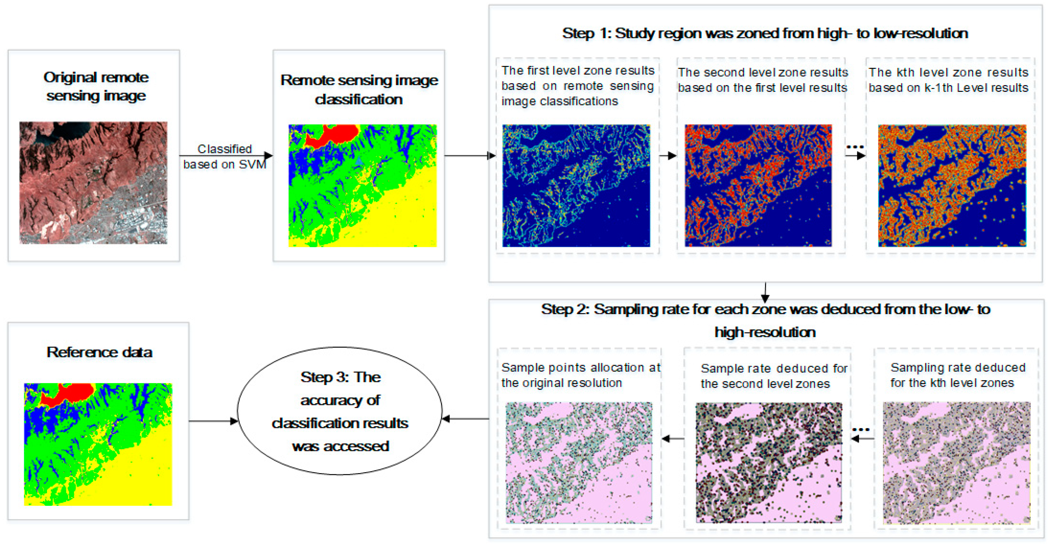
Figure 1. Overall flow of accuracy assessment of remote sensing image classification results based on the multi-level non-uniform spatial sampling method (MNSS).
Applsci 10 05568 g001
Figure 2. Step-by-step zoning of remote sensing images based on the fragmentation index.
Applsci 10 05568 g002
Figure 3. Two remote sensing images in the study region: (a) remote sensing image of the study region with 2-m spatial resolution, and (b) five categories of ground objects in the same region with 2-m spatial resolution.
Applsci 10 05568 g003
Figure 4. Classification results of the studied region.
Applsci 10 05568 g004
Figure 5. Zone results of remote sensing classification at five different spatial scales.
Applsci 10 05568 g005aApplsci 10 05568 g005b
Figure 6. Sample points distributed in the studied region.
Applsci 10 05568 g006
Figure 7. Accuracy assessment by different sampling methods.
Applsci 10 05568 g007
Figure 8. Accuracy assessment by different sampling methods.
Applsci 10 05568 g008
Table 1. Sampling rate of each zone at the fifth-level spatial resolution (162-m).
1-Zone at the Fifth Level 2-Zone at the Fifth Level3-Zone at the Fifth Level4-Zone at the Fifth Level5-Zone at the Fifth LevelTotal
Sampling rate (%)0.02761.471720.972155.531521.9971100.00
Table 2. Sampling rate of each zone at the fourth-level spatial resolution (54-m).
Zones at the fourth-level spatial resolutionSampling Rate (%)1-Zone at the Fourth Level2-Zone at the Fourth Level3-Zone at the Fourth Level4-Zone at the Fourth Level5-Zone at the Fourth Level
1-zone at the fifth level0.00310.00340.00010.00000.0000
2-zone at the fifth level0.00000.00210.00050.00000.0000
3-zone at the fifth level0.00370.00970.00390.00040.0000
4-zone at the fifth level0.05600.27860.28810.05900.0024
5-zone at the fifth level0.000049.64370.000049.64370.0000
Table 3. Sampling rate of each zone at the third-level spatial resolution (18-m).
Zones at the third-level spatial resolutionSampling Rate (%)1-Zone at the Third Level2-Zone at the Third Level3-Zone at the Third Level4-Zone at the Third Level5-Zone at the Third Level
1-zone at the
fourth level
0.03540.02880.00050.00000.0000
2-zone at the
fourth level
14.153428.32777.40320.05300.0000
3-zone at the
fourth level
0.05230.15960.07210.00850.0001
4-zone at the
fourth level
4.087020.698619.24845.40540.2637
5-zone at the
fourth level
0.00000.00000.00120.00120.0000
Table 4. Sampling rate of each zone at the second-level spatial resolution (6-m).
Zones at the second-level spatial resolutionSampling Rate (%)1-Zoneat the Second Level2-Zoneat the Second Level3-Zoneat the Second Level4-Zoneat the Second Level5-Zoneat the Second Level
1-zone at the third level11.08406.38410.84490.01500.0000
2-zone at the third level12.971629.89526.15440.19250.0011
3-zone at the third level 0.711119.72155.96260.32400.0061
4-zone at the third level0.00001.55353.66840.23950.0068
5-zone at the third level0.00010.00000.22320.04060.0000
Table 5. Sampling rate of each zone at the original spatial resolution (2-m).
Zones at the original spatial resolutionSampling Rate (%)1-Zoneat the Original Level2-Zoneat the Original Level3-Zoneat the Original Level4-Zoneat the Original Level5-Zoneat the Original Level
1-zone at the second level 15.14258.29011.29940.03550.0000
2-zone at the second level 6.715338.556011.72120.55920.0017
3-zone at the second level0.13938.60407.35030.73830.0209
4-zone at the second level0.00000.08140.59280.13450.0035
5-zone at the second level0.00000.00000.00840.00420.0014
Table 6. Accuracy assessment confusion matrix based on full inspection.
ClassificationReference Data
RoadGrassForestRoofOthersTotal
Experimental dataRoad9637291137290011939
Grass12028256711020456
Forest13809819442227053230355
Roof179313688051619212
Others126029747142691371322287
Total110903141419606167231541694249
Overall accuracy = 76.27%, Kappa = 0.6995