Data Assimilation in Spatio-Temporal Models with Non-Gaussian Initial States—The Selection Ensemble Kalman Model

Featured Application

Porosity/permeability inversion in petroleum engineering; Log-conductivity inversion with heads and tracer data in hydrogeology; Source contribution identification in air pollution monitoring.

Abstract

Assimilation of spatio-temporal data poses a challenge when allowing non-Gaussian features in the prior distribution. It becomes even more complex with nonlinear forward and likelihood models. The ensemble Kalman model and its many variants have proven resilient when handling nonlinearity. However, owing to the linearized updates, conserving the non-Gaussian features in the posterior distribution remains an issue. When the prior model is chosen in the class of selection-Gaussian distributions, the selection Ensemble Kalman model provides an approach that conserves non-Gaussianity in the posterior distribution. The synthetic case study features the prediction of a parameter field and the inversion of an initial state for the diffusion equation. By using the selection Kalman model, it is possible to represent multimodality in the posterior model while offering a 20 to 30% reduction in root mean square error relative to the traditional ensemble Kalman model.

1. Introduction

Data assimilation of spatio-temporal models is a challenge in many fields of study, including, but not limited to, air pollution mapping, weather forecast, petroleum engineering, and ground water flow assessment. Over the years, methods have been developed to handle increasingly complex problems. It started with the Kalman filter as presented in the seminal publication [1]. The Kalman filter is based on a Gaussian initial model and Gauss-linear forward and observation models. It defined the foundation for data assimilation and is still used in many assimilation studies. The extended Kalman filter (EKF) [2] appeared as a natural methodological extension that allowed for nonlinearity in the Kalman filter framework by linearization. The ensemble Kalman filter (EnKF) [3,4] defined a Monte Carlo approach to the filter and it became popular as it allowed for nonlinearity in the forward and observation models without having to evaluate analytical gradients. The EnKF and its variants have proven to be efficient in solving high-dimensional and nonlinear problems, see [5,6]. In the EnKF, the initial ensemble members represent the initial state which may not have an analytical expression. The forward model then propagates the ensemble members forward in time. Pseudo observations are generated using the observation model. The conditioning of each ensemble member is made with the Kalman weights estimated from the ensemble to give the best linear update. In cases where the initial model is non-Gaussian, the distribution of the variable of interest conditioned on the data will tend toward Gaussianity as observations are assimilated due to the linear assimilation rule.

Non-Gaussian initial distributions may be conserved by using a univariate transform into Gaussian marginals while assuming multi-Gaussianity in the transformed space. A univariate back transform is then used to return to the original space. This approach has a long history in traditional statistics, geostatistics, and more recently in ensemble methods for data assimilation, which is referred to as copulas [7], normal score transform [8], and Gaussian anamorphosis [9], respectively. The latter has shown to improve the performance of the EnKF in many applications [10,11]. There are however some unresolved issues since Gaussian anamorphosis transforms the marginal distributions rather than the full distribution, and the effect on the resulting variables interdependence is uncertain.

The Ensemble Randomized Maximum Likelihood Filter (EnRML) [12] and its close relative the Iterative EnKF (IEnKF) [6] are primarily used to handle nonlinearities in the forward and observation models, but they will also retain certain non-Gaussian features in the filtering distribution. These filters require gradient evaluations to execute the update which can be complicated even if the adjoint state method is used. One alternative is to evaluate the gradient using the ensemble itself [13], but this approach introduces an approximation with unclear consequences, particularly in models with multimodal marginals.

Multimodality in the prior model can be represented using categorical auxiliary variables to construct Gaussian mixture prior models [14,15,16]. In a spatial setting, these models appear as a combination of Gaussian random fields whose parameters depend on the value taken by the categorical variable, but in order to retain spatial dependence, the categorical variable must also have a spatial dependence. This indicator spatial variable can be modeled as a Markov [17] or truncated pluri-Gaussian [18] random field. For both of these models, there are challenges related to temporal data assimilation, although some encouraging examples have been developed [19].

We define and study an alternative prior model, the selection-Gaussian random field [20,21], which may represent multimodality, skewness, and peakedness. This random field model is conjugate with respect to Gauss-linear forward and observation models, similarly to the Gaussian random field model. The posterior distribution is therefore analytically tractable under these assumptions [22]. For general forward and observation models, ensemble based algorithms along the lines of the EnKF can be designed. Such selection ensemble Kalman algorithms are the focus of this study, and they are evaluated on a couple of examples.

In Section 2, we introduce the selection ensemble Kalman model. It provides a framework for the use of the selection-Gaussian distribution as a prior in data assimilation. This framework is then used for ensemble filtering and smoothing through the selection EnKF (SEnKF) and the selection EnKS (SEnKS) algorithms. In Section 3, a synthetic case study of the diffusion equation, with two distinct test cases, showcases the ability of the proposed approaches to assess a parameter field and the initial state of a dynamic field. Results from the SEnKF and the SEnKS are compared to that of the traditional EnKF and the EnKS, respectively. In Section 4, potential shortcomings are discussed and the results are put into perspective with respect to applicability in more realistic applications. In Section 5, conclusions are presented.

In this paper, $f(\mathit{y})$ denotes the probability density function (pdf) of a random variable $\mathit{y}$, ${\phi }_n(\mathit{y};\mathit{\mu },\Sigma )$ denotes the pdf of the Gaussian n-vector $\mathit{y}$ with expectation n-vector $\mathit{\mu }$ and covariance $(n\times n)$-matrix $\Sigma$. Furthermore, ${\Phi }_n(A;\mathit{\mu },\Sigma )$ denotes the probability of the aforementioned Gaussian n-vector $\mathit{y}$ to be in $A\subset {\mathbb{R}}^n$. We also use ${\mathit{i}}_n$ to denote the all-ones n-vector, ${\mathit{I}}_n$ to denote the identity $(n\times n)$-matrix and $\mathbf{1}(S)$ to denote the indicator function that equals 1 when S is true and 0 otherwise. We consider log-diffusivity to be an adimensional quantity and it will therefore not be given a unit.

2. Materials and Methods

Consider the unknown temporal n-vector ${\mathit{r}}_t$ for $t\in {\mathcal{T}}_r:\{0,1,\dots ,T,T+1\}$. Let $\mathit{r}=\{{\mathit{r}}_0,{\mathit{r}}_1,\dots ,{\mathit{r}}_T,{\mathit{r}}_{T+1}\}$ denote the variable of interest and let ${\mathit{r}}_{i:j}$ denote $\{{\mathit{r}}_i,{\mathit{r}}_{i+1},\dots ,{\mathit{r}}_j\},\forall (i,j)\in {\mathcal{T}}_r^2,i\le j$. Assume that the temporal m-vectors of observations ${\mathit{d}}_t$ for $t\in {\mathcal{T}}_d:\{0,1,\dots ,T\}$ are available, and define $\mathit{d}=\{{\mathit{d}}_0,{\mathit{d}}_1,\dots ,{\mathit{d}}_T\}$ and ${\mathit{d}}_{i:j}=({\mathit{d}}_i,\dots ,{\mathit{d}}_j\}$ accordingly. The model specified hereafter defines a hidden Markov (HM) model [23] as displayed in Figure 1.

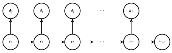
Figure 1. Graph of the hidden Markov model.

Prior model: The prior model on $\mathit{r}$ consists of an initial and a forward model,

$$\begin{array}{c}f(\mathit{r})=f({\mathit{r}}_0)f({\mathit{r}}_{1:T+1}|{\mathit{r}}_0),\end{array}$$

(1)

where $f({\mathit{r}}_0)$ is the pdf of the initial state and $f({\mathit{r}}_{1:T+1}|{\mathit{r}}_0)$ defines the forward model.

(a) Initial distribution: The distribution for the initial state $f({\mathit{r}}_0)$ is assumed to be in the class of selection-Gaussian distributions [20,21]. Consider a Gaussian $(n+n)$-vector $[\tilde{\mathit{r}},\mathit{\nu }]$,

$$\begin{array}{c}\left[\begin{array}{c}\tilde{\mathit{r}}\\ \mathit{\nu }\end{array}\right]\sim {\phi }_{2n}\left(\left[\begin{array}{c}\tilde{\mathit{r}}\\ \mathit{\nu }\end{array}\right];\left[\begin{array}{c}{\mathit{\mu }}_{\tilde{r}}\\ {\mathit{\mu }}_{\nu }\end{array}\right],\left[\begin{array}{cc}{\Sigma }_{\tilde{r}}& {\Sigma }_{\tilde{r}}{\Gamma }_{\nu |\tilde{r}}^T\\ {\Gamma }_{\nu |\tilde{r}}{\Sigma }_{\tilde{r}}& {\Sigma }_{\nu }\end{array}\right]\right),\end{array}$$

(2)

with n-vectors ${\mathit{\mu }}_{\tilde{r}}$ and ${\mathit{\mu }}_{\nu }$, $(n\times n)$-matrix ${\Gamma }_{\nu |\tilde{r}}$, and where ${\Sigma }_{\tilde{r}}$, ${\Sigma }_{\nu }$, and ${\Sigma }_{\nu |\tilde{r}}$ are all three covariance $(n\times n)$-matrices with ${\Sigma }_{\nu }={\Gamma }_{\nu |\tilde{r}}{\Sigma }_{\tilde{r}}{\Gamma }_{\nu |\tilde{r}}^T+{\Sigma }_{\nu |\tilde{r}}$. Define a selection set $A\subset {\mathbb{R}}^n$ of dimension n and let ${\mathit{r}}_0=[\tilde{\mathit{r}}|\mathit{\nu }\in A]$; then, ${\mathit{r}}_0$ is in the class of selection-Gaussian distribution and its pdf is,

$$\begin{array}{cc}\hfill f({\mathit{r}}_0)=& {\left[{\Phi }_n(A;{\mathit{\mu }}_{\nu },{\Sigma }_{\nu })\right]}^{-1}\hfill \\ \hfill \times & {\Phi }_n(A;{\mathit{\mu }}_{\nu }+{\Gamma }_{\nu |\tilde{r}}({\mathit{r}}_0-{\mathit{\mu }}_{\tilde{r}}),{\Sigma }_{\nu |\tilde{r}})\times {\phi }_n({\mathit{r}}_0;{\mathit{\mu }}_{\tilde{r}},{\Sigma }_{\tilde{r}}).\hfill \end{array}$$

(3)

Note that the class of Gaussian distributions constitutes a subset of the class of selection-Gaussian distributions with ${\Gamma }_{\nu |\tilde{r}}=0\times {\mathit{I}}_n$. The dependence in $[\tilde{\mathit{r}},\mathit{\nu }]$ represented by ${\Gamma }_{\nu |\tilde{r}}$ and the selection subset A are crucial user-defined parameters with the latter being temporally constant. The selection-Gaussian model may represent multimodal, skewed, and/or peaked marginal distributions, see [21]. In this study, the initial distribution is defined to be a discretized stationary selection-Gaussian random field with parametrization,

$$\begin{array}{cc}\hfill {\mathit{\mu }}_{\tilde{r}}=& {\mu }_{\tilde{r}}{\mathit{i}}_n\hfill \\ \hfill {\mathit{\mu }}_{\nu }=& {\mu }_{\nu }{\mathit{i}}_n\hfill \\ \hfill {\Sigma }_{\tilde{r}}=& {\sigma }_{\tilde{r}}^2{\Sigma }_{\tilde{r}}^{\rho }\hfill \\ \hfill {\Sigma }_{\nu }=& {\gamma }^2{\Sigma }_{\tilde{r}}^{\rho }+(1-{\gamma }^2){\mathit{I}}_n\hfill \\ \hfill {\Gamma }_{\nu |\tilde{r}}=& \gamma {\sigma }_{\tilde{r}}^{-1}{\mathit{I}}_n.\hfill \end{array}$$

(4)

For a given spatial correlation $(n\times n)$-matrix ${\Sigma }_{\tilde{r}}^{\rho }$, a stationary selection-Gaussian random field is fully parametrized by ${\mathbf{\Theta }}^{SG}=({\mu }_{\tilde{r}},{\mu }_{\nu },{\sigma }_{\tilde{r}},{\Sigma }_{\tilde{r}}^{\rho },\gamma ,A)$. Similarly, a stationary Gaussian random field is parametrized by ${\mathbf{\Theta }}^G=({\mu }_r,{\sigma }_r,{\Sigma }_r^{\rho })$.

(b) Forward model: The forward model given the initial state $[{\mathit{r}}_{1:T+1}|{\mathit{r}}_0]$ is defined as

$$\begin{array}{c}\hfill f({\mathit{r}}_{1:T+1}|{\mathit{r}}_0)=\prod _{t=0}^{T}f({\mathit{r}}_{t+1}|{\mathit{r}}_t),\end{array}$$

(5)

with

$$\begin{array}{cc}\hfill [{\mathit{r}}_{t+1}|{\mathit{r}}_t]=& {\omega }_t({\mathit{r}}_t,{\mathit{ϵ}}_t^r)\sim f({\mathit{r}}_{t+1}|{\mathit{r}}_t),\hfill \end{array}$$

(6)

where ${\omega }_t(·,·)\in {\mathbb{R}}^n$ is the forward model with random n-vector ${\mathit{ϵ}}_t^r$, independent and identically distributed (iid) for each t. This forward model may be nonlinear, but, since it only involves the variable at the previous time step ${\mathit{r}}_t$, it defines a first-order Markov chain. Note that $f({\mathit{r}}_{t+1}|{\mathit{r}}_t)$ cannot generally be written in closed form.

Likelihood model: The likelihood model for $[\mathit{d}|\mathit{r}]$ is defined as conditional independent with single-site response,

$$\begin{array}{c}\hfill f(\mathit{d}|\mathit{r})=\prod _{t=0}^{T}f({\mathit{d}}_t|{\mathit{r}}_t),\end{array}$$

(7)

with

$$\begin{array}{cc}\hfill [{\mathit{d}}_t|{\mathit{r}}_t]=& {\psi }_t({\mathit{r}}_t,{\mathit{ϵ}}_t^d)\sim f({\mathit{d}}_t|{\mathit{r}}_t),\hfill \end{array}$$

(8)

where ${\psi }_t(·,·)\in {\mathbb{R}}^m$ is the likelihood function with random m-vector ${\mathit{ϵ}}_t^d$, iid for each t. Note that $f({\mathit{d}}_t|{\mathit{r}}_t)$ cannot generally be written in closed form.

Posterior model: The posterior model for the HM model in Figure 1 is given by

$$\begin{array}{cc}\hfill [\mathit{r}|\mathit{d}]\sim f(\mathit{r}|\mathit{d})=& const\times f(\mathit{d}|\mathit{r})f(\mathit{r})\hfill \\ \hfill =& const\times f({\mathit{d}}_0|{\mathit{r}}_0)f({\mathit{r}}_0)\prod _{t=1}^{T}f({\mathit{d}}_t|{\mathit{r}}_t)f({\mathit{r}}_t|{\mathit{r}}_{t-1})f({\mathit{r}}_{T+1}|{\mathit{r}}_T)\hfill \\ \hfill =& f({\mathit{r}}_0|\mathit{d})\prod _{t=1}^{T}f({\mathit{r}}_t|{\mathit{r}}_{t-1},{\mathit{d}}_{t:T})f({\mathit{r}}_{T+1}|{\mathit{r}}_T),\hfill \end{array}$$

(9)

and is also a Markov chain, see [23,24]. This model is denoted the selection ensemble Kalman model. If the forward and likelihood models are Gauss-linear, the posterior model is also selection-Gaussian and analytically tractable, see [22]. When the forward and/or likelihood models are nonlinear, however, approximate or sampling based assessment of the posterior model must be made. For this purpose, we introduce the selection ensemble Kalman filter (SEnKF) and smoother (SEnKS) in the spirit of the traditional ensemble Kalman model [3].

The traditional EnKF algorithm aims at assessing the forecast pdf $f({\mathit{r}}_{T+1}|{\mathit{d}}_{0:T})$, and it is justified by general HM model recursions, see [23]. The algorithm is initiated by

$$\begin{array}{c}\hfill [{\mathit{r}}_1|{\mathit{d}}_0]\sim f({\mathit{r}}_1|{\mathit{d}}_0)=\int f({\mathit{r}}_1|{\mathit{r}}_0){[f({\mathit{d}}_0)]}^{-1}f({\mathit{d}}_0|{\mathit{r}}_0)f({\mathit{r}}_0)\mathrm{d}{\mathit{r}}_0,\end{array}$$

(10)

and utilizes the recursion for $t=1,\dots ,T$,

$$\begin{array}{c}\hfill [{\mathit{r}}_{t+1}|{\mathit{d}}_{0:t}]\sim f({\mathit{r}}_{t+1}|{\mathit{d}}_{0:t})=\int f({\mathit{r}}_{t+1}|{\mathit{r}}_t){[f({\mathit{d}}_t|{\mathit{d}}_{0:t-1})]}^{-1}f({\mathit{d}}_t|{\mathit{r}}_t)f({\mathit{r}}_t|{\mathit{d}}_{0:t-1})\mathrm{d}{\mathit{r}}_t.\end{array}$$

(11)

The expressions are represented by an ensemble of realizations, which in each recursion is conditioned using a linearized approximation with Kalman weights estimated from the ensemble. Thereafter, the ensemble is forwarded to the next time step. The SEnKF introduced in this study relies on the same relations as above, but it operates on the augmented $(n+n)$-vector $[{\tilde{\mathit{r}}}_{·},\mathit{\nu }]$, see Equation (2). Hence, the forward model is defined as

$$\begin{array}{c}\left[\begin{array}{c}{\tilde{\mathit{r}}}_{t+1}\\ {\mathit{\nu }}_{t+1}\end{array}\right|\left.\begin{array}{c}{\tilde{\mathit{r}}}_t\\ {\mathit{\nu }}_t\end{array}\right]=\left[\begin{array}{c}{\omega }_t({\tilde{\mathit{r}}}_t,{ϵ}_t^r)\\ {\mathit{\nu }}_t\end{array}\right].\end{array}$$

(12)

where the auxiliary n-vector ${\nu }_t$ is temporally constant.

The likelihood model is defined as

$$\begin{array}{c}\left[\begin{array}{c}\\ {\mathit{d}}_t\\ \end{array}\right.\left|\begin{array}{c}{\tilde{\mathit{r}}}_t\\ \\ {\mathit{\nu }}_t\end{array}\right]={\psi }_t({\tilde{\mathit{r}}}_t,{ϵ}_t^d).\end{array}$$

(13)

The SEnKF algorithm provides an ensemble representation of

$$\begin{array}{c}\left[\begin{array}{c}{\tilde{\mathit{r}}}_{T+1}\\ \\ \mathit{\nu }\end{array}\right|\left.\begin{array}{c}\\ {\mathit{d}}_{0:T}\\ \end{array}\right]\sim f({\tilde{\mathit{r}}}_{T+1},\mathit{\nu }|{\mathit{d}}_{0:T}),\end{array}$$

(14)

and, based on this ensemble, empirical sampling based inference, see [21], is used to obtain the forecast of interest:

$$\begin{array}{c}[{\mathit{r}}_{T+1}|{\mathit{d}}_{0:T}]\sim f({\mathit{r}}_{T+1}|{\mathit{d}}_{0:T})=f({\tilde{\mathit{r}}}_{T+1}|{\mathit{d}}_{0:T},\mathit{\nu }\in A).\end{array}$$

(15)

The SEnKF algorithm is specified in Algorithm A1 in Appendix A.

The traditional EnKS algorithm aims at evaluating the interpolation pdf $f({\mathit{r}}_{0:T}|{\mathit{d}}_{0:T})$ with corresponding HM model recursions, see [23]. The algorithm is initiated by

$$\begin{array}{c}\hfill [{\mathit{r}}_0|{\mathit{d}}_0]\sim f({\mathit{r}}_0|{\mathit{d}}_0)={[f({\mathit{d}}_0)]}^{-1}f({\mathit{d}}_0|{\mathit{r}}_0)f({\mathit{r}}_0),\end{array}$$

(16)

and the recursions for $t=1,\dots ,T$,

$$\begin{array}{cc}\hfill [{\mathit{r}}_{0:t}|{\mathit{d}}_{0:t}]\sim & f({\mathit{r}}_{0:t}|{\mathit{d}}_{0:t})\hfill \\ \hfill =& {[f({\mathit{d}}_t|{\mathit{d}}_{0:t-1})]}^{-1}f({\mathit{d}}_t|{\mathit{r}}_{0:t},{\mathit{d}}_{0:t-1})f({\mathit{r}}_t|{\mathit{r}}_{0:t-1},{\mathit{d}}_{0:t-1})f({\mathit{r}}_{0:t-1}|{\mathit{d}}_{0:t-1})\hfill \\ \hfill =& {[f({\mathit{d}}_t|{\mathit{d}}_{0:t-1})]}^{-1}f({\mathit{d}}_t|{\mathit{r}}_t)f({\mathit{r}}_t|{\mathit{r}}_{t-1})f({\mathit{r}}_{0:t-1}|{\mathit{d}}_{0:t-1}).\hfill \end{array}$$

(17)

The expressions are represented by an ensemble of realizations. Forwarding is made on the ensemble and the conditioning is empirically linearized. Note that the dimension of the model increases very fast, one may therefore only store the interpolation pdf $f({\mathit{r}}_s|{\mathit{d}}_{0:T})$ at the time point s of interest. The SEnKS introduced in this study relies on the relations defined above and uses an extended $(n+n)$-vector $[\tilde{\mathit{r}},\mathit{\nu }]$ as defined in Equation (2). The forward and likelihood models are identical to those defined for the filter. The SEnKS algorithm provides an ensemble representation of

$$\begin{array}{c}\left[\begin{array}{c}{\tilde{\mathit{r}}}_{0:T}\\ \\ \mathit{\nu }\end{array}\right|\left.\begin{array}{c}\\ {\mathit{d}}_{0:T}\\ \end{array}\right]\sim f({\tilde{\mathit{r}}}_{0:T},\mathit{\nu }|{\mathit{d}}_{0:T}),\end{array}$$

(18)

and by using empirical sampling based inference, see [21], the interpolation of interest is assessed,

$$\begin{array}{c}[{\mathit{r}}_{0:T}|{\mathit{d}}_{0:T}]\sim f({\mathit{r}}_{0:T}|{\mathit{d}}_{0:T})=f({\tilde{\mathit{r}}}_{0:T}|{\mathit{d}}_{0:T},\mathit{\nu }\in A).\end{array}$$

(19)

The SEnKS algorithm is specified in Algorithm A2 in the Appendix A. Both algorithms, SEnKF and SEnKS, contain empirically linearized conditioning and asymptotic results, when the ensemble size goes to infinity, and are consistent only for Gauss-linear forward and likelihood models. Under these assumptions, the model is analytically tractable; however, see [22]. In spite of this lack of asymptotic consistency for general HM models, the ensemble Kalman scheme has proven surprisingly reliable for high-dimensional, weakly nonlinear models even with very modest ensemble sizes [25].

3. Results

We consider two test cases to illustrate the relevance of the selection ensemble Kalman algorithms presented in Section 2. The model, common to both test cases, is based on the diffusion equation. The test cases are designed such that it will be opportune to consider bi-modal initial distributions. In the first test case, we compare the SEnKF to the traditional EnKF with a focus on predicting the diffusivity field that contains a high diffusivity channel. In the second test case, we compare the SEnKS to the traditional EnKS with a focus on evaluating the initial temperature field that is divided into two distinct areas where the initial temperature is substantially higher in one than in the other.

3.1. Model

Consider a discretized spatio-temporal random field, $\{r_t(\mathit{x}),\mathit{x}\in {\mathcal{L}}_r\subset {\mathbb{R}}^2\}$ where $t\in {\mathcal{L}}_t:\{0,1,.\dots ,T\}$ and $r_t(·)\in \mathbb{R}$ that represents temperature (${}^{\circ }$C). Let a discretized spatial random field, $\{\lambda (\mathit{x}),\mathit{x}\in {\mathcal{L}}_r\subset {\mathbb{R}}^2\}$; with $\lambda (·)\in {\mathbb{R}}_{\oplus }$ representing diffusivity (${\mathrm{m}}^2.{\mathrm{s}}^{-1}$). Let $\mathit{x}$ be the spatial reference on the regular spatial grid ${\mathcal{L}}_r$ on the domain D, while t is the temporal reference on the regular temporal grid ${\mathcal{L}}_t$. The number of spatial grid nodes is $n=21\times 21$, and they are placed every 10 cm vertically and horizontally. The discretized temperature field at time t may be represented by the n-vector ${\mathit{r}}_t$ and the diffusivity field by the n-vector $\mathit{\lambda }$. Both are assumed to be unknown. Note that the Kalman models are defined on the joint variable $[{\mathit{r}}_t,\mathit{\lambda }]$.

Assume that, given the initial temperature field, the field evolves according to the diffusion equation:

$$\begin{array}{cc}\hfill \frac{\partial r_t(\mathit{x})}{\partial t}-\nabla ·(\lambda (\mathit{x})\nabla r_t(\mathit{x}))=& q\hfill \\ \hfill \nabla r_t(\mathit{x})·\mathit{n}=& 0,\hfill \end{array}$$

(20)

with $\mathit{n}$ the outer normal to the domain and q a source term. The expression in Equation (20) is discretized using finite differences and the forward model is defined as

$$\begin{array}{cc}\hfill [{\mathit{r}}_{t+1}|{\mathit{r}}_t,\mathit{\lambda }]=& {\omega }^{*}({\mathit{r}}_t,\mathit{\lambda }),\hfill \end{array}$$

(21)

with ${\omega }^{*}(·,·)\in {\mathbb{R}}^n$. Convergence and stability of the numerical method are easily ensured for the finite difference scheme that is used. The initial temperature field ${\mathit{r}}_0$ is considered unknown in the test cases.

The forward model is assumed to be perfect in the sense that there is no model error. The forward model in Equation (6) then takes the form,

$$\begin{array}{c}\hfill \omega ([{\mathit{r}}_t,\mathit{\lambda }],0{\mathit{i}}_n)=\left[\begin{array}{c}{\omega }^{*}({\mathit{r}}_t,\mathit{\lambda })\\ \mathit{\lambda }\end{array}\right].\end{array}$$

(22)

This forward model is nonlinear due to the product of ${\mathit{r}}_t$ and $\mathit{\lambda }$ in Equation (20). Consequently, the assumption of Gauss-linearity required for both the traditional Kalman model [1] and the selection Kalman model [22] is violated and necessitates ensemble based algorithms.

The observations are acquired in a $m=5$ location pattern on the spatial grid ${\mathcal{L}}_r$ at each temporal node in ${\mathcal{L}}_t$, providing the set of observations m-vectors ${\mathit{d}}_t$, $t\in {\mathcal{L}}_t$. The corresponding likelihood model is defined as

$$\begin{array}{cc}\hfill [{\mathit{d}}_t|{\mathit{r}}_t]={\psi }_t({\mathit{r}}_t,{\mathit{ϵ}}_t^d)=& \mathit{H}{\mathit{r}}_t+{\mathit{ϵ}}_t^d\hfill \\ \hfill f({\mathit{d}}_t|{\mathit{r}}_t)=& {\phi }_m({\mathit{d}}_t;\mathit{H}{\mathit{r}}_t,{\Sigma }_{d|r}),\hfill \end{array}$$

(23)

where the observation $(m\times n)$-matrix $\mathit{H}$ is a binary selection matrix, while the centered Gaussian m-vector ${\mathit{ϵ}}_t^d$ with the covariance $(m\times m)$-matrix ${\Sigma }_{d|r}={\sigma }_{d|r}^2{\mathit{I}}_m$, and ${\sigma }_{d|r}^2=0.1$ represents independent observation errors. This likelihood model is in Gauss-linear form.

3.2. Test Case 1: Predicting the Parameter Field

The focus of this test case is to predict the unknown diffusivity field $\mathit{\lambda }$ based on the observations $\mathit{d}$. Because diffusivity is constant in time, smoothing and filtering give an identical prediction of the field. However, filtering is preferred because it does not require updating the ensemble at all future times in addition to the previous one, see [26]. The posterior model is evaluated using the SEnKF, see Appendix A and the results are compared to those from the traditional EnKF algorithm.

The true diffusivity n-vector $\mathit{\lambda }$ is displayed in Figure 2. The diffusivity $\mathit{\lambda }$ is always positive. To ensure that ensemble updates do not lead to negative diffusivity values, we work on $log(\mathit{\lambda })$. The figure shows a channel in which the diffusivity is higher than in the rest of the field. The diffusivity field is formally defined as

$$\begin{array}{c}\hfill \mathit{\lambda }(\mathit{x})={\lambda }_1\mathbf{1}(\mathit{x}\in D_1)+{\lambda }_2\mathbf{1}(\mathit{x}\in D_2),\end{array}$$

(24)

where $D_1\subset D$ is the low diffusivity area and $D_2\subset D$ is the high diffusivity channel. The parameter values are ${\lambda }_1=e^{-12}{\mathrm{m}}^2.{\mathrm{s}}^{-1}$ and ${\lambda }_2=e^{-5}{\mathrm{m}}^2.{\mathrm{s}}^{-1}$. The true temperature field is initially at $20{}^{\circ }$C and the heat source on the lower border of the high diffusivity channel starts pumping in heat at $T=0$ at a constant volumetric rate $q=15\mathrm{W} {\mathrm{m}}^{-3}$, see Figure 2. The temporal evoluation of the temperature field, shown in Figure 3, is obtained by solving the diffusion equation in Equation (20) for the log-diffusivity field in Figure 2 and the initial temperature field defined above. The temperature observations $\mathit{d}$, see Figure 4, are then collected from the five locations shown in Figure 2 using the likelihood model defined in Equation (23). The measurements are taken every second from $T=0$ to $T=100$. As the heat from the source diffuses mostly along the high diffusivity channel, the observed temperature increases substantially at observation locations within the channel.

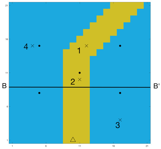
Figure 2. Initial log-diffusivity field with observation locations $·$, monitoring locations ×, and heat source ∆.

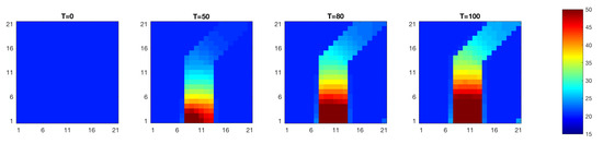
Figure 3. True temperature (${}^{\circ }$C) field evolution over time.

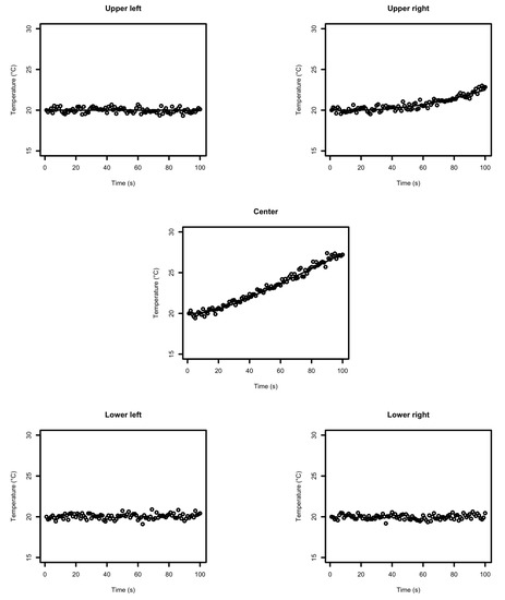
Figure 4. Data collected over time ($·$) and true temperature evolution (line) at the data collection points.

The unknown initial field for log-diffusivity $log(\mathit{\lambda })$ is assigned a stationary selection-Gaussian random field prior model with parameters ${\mathbf{\Theta }}_{\lambda }^{SG}=({\mu }_{\tilde{r}}^{\lambda },{\mu }_{\nu }^{\lambda },{\sigma }_{\tilde{r}}^{\lambda },{\Sigma }_{\tilde{r}}^{\rho },{\gamma }^{\lambda },A)$, see [21] and Equation (2). The parameter values for the prior model are listed in Table 1.

Table 1. Parameter values for the selection-Gaussian initial distribution for the initial log-diffusivity field.

Parameters	Values
${\mu }_{\tilde{r}}^{\lambda }$	$-8.5$
${\mu }_{\nu }^{\lambda }$	0
${\sigma }_{\tilde{r}}^{\lambda }$	$\sqrt{1.6}$
${\gamma }^{\lambda }$	$0.9$
A	${]-\infty ,-0.3]\cup [0.5,+\infty [}^n$

The unknown initial temperature field ${\mathit{r}}_0$ is assigned a stationary Gaussian random field prior model with parameters ${\mathbf{\Theta }}_r^G=({\mu }_r,{\sigma }_r,{\Sigma }_r^{\rho })$ with expectation and variance levels ${\mu }_r=20$ and ${\sigma }_r^2=2$, respectively. The variance level is relatively large as we assume little prior knowledge of the initial temperature field. For both prior models, the spatial correlation ($n\times n$)-matrix ${\Sigma }_{·}^{\rho }$ is defined by the second order exponential spatial correlation function ${\rho }_{·}(\tau )=exp(-{\tau }^2/{\delta }^2);\delta =0.15$, with interdistance $\tau$.

Figure 5 contains realizations from the prior model of the log-diffusivity field and their associated spatial histograms. The prior model is specified to be spatially stationary except for boundary effects with bi-modal spatial histograms. The selection set $A\subset {\mathbb{R}}^n$ for the prior model is chosen to obtain bi-modal marginal distributions with a very dominant mode centered slightly above the value for ${\lambda }_1$ and a very small mode centered slightly below the value for ${\lambda }_2$. The prior is therefore not centered at the true values. Note that the joint random field $[log(\mathit{\lambda }),{\mathit{r}}_0]$ will appear as a bi-variate selection-Gaussian random field, see [21].

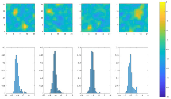
Figure 5. Realizations from the initial selection-Gaussian distribution of the log diffusivity $f(log(\mathit{\lambda }))$ at time $T=0$ (upper panels) and associated spatial histogram (lower panels). Lower panels: the horizontal axes represent the log-diffusivity, the vertical axes represent the relative prevalence of each log-diffusivity value for the realization in the panel right above.

The SEnKF operates on the $3n$-vector $[log(\tilde{\mathit{\lambda }}),\mathit{\nu },{\mathit{r}}_0]$, and therefore we generate an initial ensemble with $n_e$ = 10,000 ensemble members that are sampled from the Gaussian $3n$-vector $[log(\tilde{\mathit{\lambda }}),\mathit{\nu },{\mathit{r}}_0]$ with pdf,

$$\begin{array}{c}\left[\begin{array}{c}log(\tilde{\mathit{\lambda }})\\ \mathit{\nu }\\ {\mathit{r}}_0\end{array}\right]\sim {\phi }_{3n}\left(\left[\begin{array}{c}log(\tilde{\mathit{\lambda }})\\ \mathit{\nu }\\ {\mathit{r}}_0\end{array}\right];\left[\begin{array}{c}{\mathit{\mu }}_{\tilde{r}}^{\lambda }\\ {\mathit{\mu }}_{\nu }^{\lambda }\\ {\mathit{\mu }}_r\end{array}\right],\left[\begin{array}{ccc}{{\sigma }_{\tilde{r}}^{\lambda }}^2{\Sigma }_{\tilde{r}}^{\rho }& {\gamma }^{\lambda }{\sigma }_{\tilde{r}}^{\lambda }{{\Sigma }_{\tilde{r}}^{\rho }}^T& 0\\ {\gamma }^{\lambda }{\sigma }_{\tilde{r}}^{\lambda }{\Sigma }_{\tilde{r}}^{\rho }& {{\gamma }^{\lambda }}^2{\Sigma }_{\tilde{r}}^{\rho }+(1-{{\gamma }^{\lambda }}^2){\mathit{I}}_n& 0\\ 0& 0& {{\sigma }_r}^2{\Sigma }_r^{\rho }\end{array}\right]\right).\end{array}$$

(25)

The EnKF operates on the $2n$-vector $[log(\mathit{\lambda }),{\mathit{r}}_0]$, and therefore we generate an initial ensemble with $n_e$ = 10,000 ensemble members that are sampled from the selection-Gaussian distribution $f(log(\mathit{\lambda }),{\mathit{r}}_0)$. The variables $log(\mathit{\lambda })$ and ${\mathit{r}}_0$ are independent, so we generate them independently: 10,000 samples from the selection-Gaussian n-vector $log(\mathit{\lambda })$ with parameters ${\mathbf{\Theta }}_{\lambda }^{SG}$ and 10,000 samples from the Gaussian n-vector ${\mathit{r}}_0$ with parameters ${\mathbf{\Theta }}_r^G$. It is important to understand that both ensemble algorithms are initiated with an ensemble from an identical selection-Gaussian random field prior model for $[log(\lambda ),{\mathit{r}}_0]$ at $T=0$, which reflects the bi-modality of the prior model. Due to the size of the ensemble relative to the dimension of the problem, we are using neither localization nor inflation in the algorithms.

To illustrate the differences between the SEnKF and the EnKF, we present the following results for both algorithms:

• The marginal posterior distributions $f(log({\lambda }_i)|{\mathit{d}}_{0:T})$ of the log-diffusivity field at four monitoring locations denoted $1,2,3,4$ on Figure 2, at time $T=0,50,80,100$.
• The marginal maximum a posteriori (MMAP) prediction of the log-diffusivity field at time at time $T=0,50,80,100$.
• Realizations from the posterior distribution $f(log(\mathit{\lambda })|{\mathit{d}}_{0:T})$ at time $T=100$.
• The root mean square errors (RMSE) of the MMAP prediction of the log-diffusivity field relative to the true log-diffusivity field at time $T=100$.

Figure 6 and Figure 7 show the marginal posterior pdfs $f(log({\lambda }_i)|{\mathit{d}}_{0:T})$ at the four monitoring locations at time $T=0,50,80,100$ for the SEnKF and EnKF algorithms, respectively. Monitoring locations 1 and 2 are placed within the high diffusivity area while the two other locations are placed far into the low diffusivity area. At $T=0$, all pdfs are identical, in all locations due to the stationary prior model and for both algorithms due to identical prior models. The SEnKF results appear to preserve bi-modality as observations are assimilated. As more data are made available, the high value mode increases at monitoring locations 1 and 2 that are inside the high diffusivity area. The low value mode remains dominant at monitoring locations within the low diffusivity areas. These results reflect expected behaviors. The traditional EnKF results are significantly different since the bi-modality of the marginal pdfs disappears already at $T=50$. The marginal pdfs are Gaussian-like and are gently moved toward high and low values depending on which diffusivity area the monitoring locations are in. This regression toward the mean effect of the EnKF is generally recognized as it gives the best prediction in the squared error sense [27].

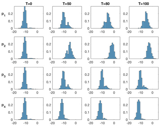
Figure 6. SEnKF approach: Marginal posterior distribution of the log diffusivity $f(log({\lambda }_i)|{\mathit{d}}_{0:T})$ at time $T=0,50,80,100$ at the monitoring locations ($1,2,3,4$) denoted ($p_1,p_2,p_3,p_4$).

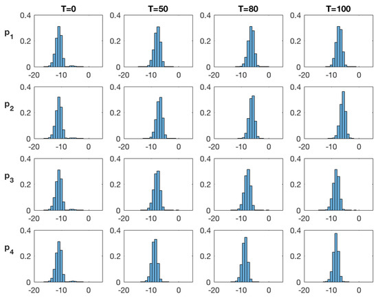
Figure 7. EnKF approach: Marginal posterior distribution of the log diffusivity $f(log({\lambda }_i)|{\mathit{d}}_{0:T})$ at time $T=0,50,80,100$ at the monitoring locations ($1,2,3,4$) denoted ($p_1,p_2,p_3,p_4$).

Figure 8 displays the MMAP predictions based on the SEnKF and the traditional EnKF at time $T=0,50,80,100$. At $T=0$, the predictions from the two algorithms are identical since they use identical prior models. As observations are assimilated, the SEnKF predictions reproduce the high diffusivity area relatively well, with clear contrast. The traditional EnKF predictions also indicate the diffusivity areas, but with less contrast. Figure 9 displays the MMAP prediction at $T=100$ along the section B-B’ shown in Figure 2. The high contrast reliable reconstruction of the high diffusivity channel by the SEnKF algorithm is confirmed. The traditional EnKF predictions appear less reliable. The $80\%$ highest density interval (HDI) [28] covers the true diffusivity values for the SEnKF while these values are far outside the interval for the traditional EnKF results. The results are consistent with the observations made regarding the marginal posterior pdfs in Figure 6 and Figure 7.

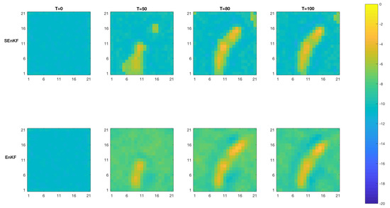
Figure 8. MMAP predictions of the log diffusivity field $(log(\mathit{\lambda })|{\mathit{d}}_{0:T})$ at time $T=0,50,80,100$ (upper panels—SEnKF approach, lower panels—EnKF approach).

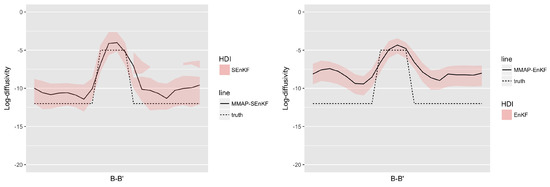
Figure 9. MMAP predictions of the log diffusivity field with $80\%$ HDI in cross section B-B’ at time $T=100$ with SEnKF (left) and with EnKF (right).

Figure 10 and Figure 11 show realizations and spatial histograms from the posterior distribution of the log-diffusivity at time $T=100$ for the SEnKF and traditional EnKF algorithms, respectively. The realizations from the SEnKF largely reproduce the channel with clear contrast while the realizations from the EnKF also reproduce the channel, but with much less contrast. The spatial histograms also underline the difference in contrast in that they are clearly bi-modal for the SEnKS and much more Gaussian-like for the EnKS.

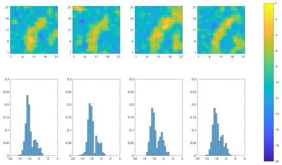
Figure 10. SEnKF approach: Realizations of the posterior distribution of the log diffusivity $f(log(\mathit{\lambda })|{\mathit{d}}_{0:T})$ at time $T=100$ (upper panels) and associated spatial histogram (lower panels). Lower panels: the horizontal axes represent the log-diffusivity, the vertical axes represent the relative prevalence of each log-diffusivity value for the realization in the panel right above.

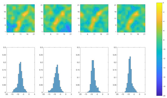
Figure 11. EnKF approach: Realizations of the posterior distribution of the log diffusivity $f(log(\mathit{\lambda })|{\mathit{d}}_{0:T})$ at time $T=100$ (upper panels) and associated spatial histogram (lower panels). Lower panels: the horizontal axes represent the log-diffusivity, the vertical axes represent the relative prevalence of each log-diffusivity value for the realization in the panel right above.

Table 2 shows that the RMSE of the MMAP prediction relative to the true diffusivity field for the SEnKF is approximately 30% lower than for the EnKF.

Table 2. RMSE comparing the MMAP prediction and the true log diffusivity field at time $T=100$.

	SEnKF	ENKF
$RMS{E}_{T=100}$	2.72	3.76

This test case clearly illustrates the SEnKF’s ability to conserve multimodality in the posterior distribution and it leads to predictions with better constrast and accuracy. We conclude that the reconstruction of the true diffusivity field is done more reliably by the SEnKF algorithm than by the EnKF algorithm.

3.3. Test Case 2: Reconstructing the Initial Field

The focus of the study is to evaluate the unknown initial state of the temperature field ${\mathit{r}}_0$ based on the observations $\mathit{d}$. The posterior model $f({\mathit{r}}_0|\mathit{d})$ is assessed using the SEnKS, see Appendix A, and the results are compared to those from the traditional EnKS.

The true initial temperature field ${\mathit{r}}_0$ is set at 20 ${}^{\circ }$C except for a square shaped region with temperature set at 45 ${}^{\circ }$C, see Figure 12. The temperature field is formally defined as

$$\begin{array}{c}\hfill {\mathit{r}}_0(\mathit{x})={\tau }_1\mathbf{1}(\mathit{x}\in D_1)+{\tau }_2\mathbf{1}(\mathit{x}\in D_2),\end{array}$$

(26)

where $D_1\subset D$ is the low temperature area and $D_2\subset D$ is the high temperature area, and ${\tau }_1$ = 20 ${}^{\circ }$C and ${\tau }_2$ = 45 ${}^{\circ }$C. Figure 12 shows the true log-diffusivity n-vector $log(\mathit{\lambda })$. The diffusivity $\mathit{\lambda }$ is always positive. To ensure that ensemble updates do not lead to negative diffusivity values, we work on $log(\mathit{\lambda })$. The heat contained in the high temperature area will diffuse towards the rest of the field according to the diffusion equation in Equation (20), see Figure 13. The temporal observations are collected at five different observation locations according to the likelihood model in Equation (23), see Figure 12. Figure 14 displays the observations $\mathit{d}$ where it is clear that the observed temperature increases substantially only at the observation locations close to the high temperature area. The measurements are taken every second from T = 0 to T = 50.

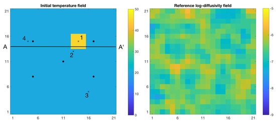
Figure 12. Initial temperature (${}^{\circ }$C) field (left) with data collection points $·$ and monitoring locations × and reference log-diffusivity field (right).

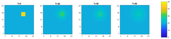
Figure 13. True temperature (${}^{\circ }$C) field evolution over time.

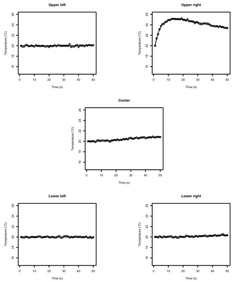
Figure 14. Data collected over time (points) and true temperature (${}^{\circ }$C) evolution at the data collection points (line).

The unknown initial temperature field ${\mathit{r}}_0$ is assigned a stationary selection-Gaussian random field prior model with parameters ${\mathbf{\Theta }}_r^{SG}=({\mu }_{\tilde{r}},{\mu }_{\nu },{\sigma }_{\tilde{r}},{\Sigma }_{\tilde{r}}^{\rho },\gamma ,A)$. The parameter values are listed in Table 3. The unknown log-diffusivity field $log(\mathit{\lambda })$ is assigned a stationary Gaussian random field prior model with parameters ${\mathbf{\Theta }}_{\lambda }^G=({\mu }_{\lambda },{\sigma }_{\lambda },{\Sigma }_{\lambda }^{\rho })$ with expectation and variance levels ${\mu }_{\lambda }=-8.5$ and ${\sigma }_{\lambda }^2=2$, respectively. For both prior models, the spatial correlation ($n\times n$)-matrix ${\Sigma }_{·}^{\rho }$ is defined by the second order exponential spatial correlation function ${\rho }_{·}(\tau )=exp(-{\tau }^2/{\delta }^2);\delta =0.15$, with interdistance $\tau$.

Table 3. Parameter values for the selection-Gaussian initial distribution for the initial temperature prior model.

Parameters	Values
${\mu }_{\tilde{r}}$	$28.75$
${\mu }_{\nu }$	0
${\sigma }_{\tilde{r}}$	$\sqrt{10}$
$\gamma$	$0.8$
A	${]-\infty ,-0.2]\cup [0.5,+\infty [}^n$

Figure 15 contains four realizations from the prior model of the temperature field and their spatial histograms. The marginal initial distributions of the realizations are bi-modal and spatially stationary except for boundary effects. The selection set $A\subset {\mathbb{R}}^n$ in the prior model is chosen to obtain a bi-modal marginal distribution with one large mode approximately centered about 20 ${}^{\circ }$C and a smaller mode centered close to 45 ${}^{\circ }$C.

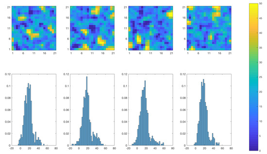
Figure 15. Realizations from the selection-Gaussian initial distribution of the initial temperature field $f({\mathit{r}}_0)$ at time $T=0$ (upper panels) and associated spatial histogram (lower panels). Upper panels: the colorbar gives the temperature in ${}^{\circ }$C. Lower panels: the horizontal axes represent the temperature (${}^{\circ }$C), the vertical axes represent the relative prevalence of each temperature value for the realization right above.

The SEnKS operates on the $3n$-vector $[{\tilde{\mathit{r}}}_0,\mathit{\nu },log(\mathit{\lambda })]$, and therefore we generate an initial ensemble with $n_e$ = 10,000 ensemble members that are sampled from the Gaussian $3n$-vector $[{\tilde{\mathit{r}}}_0,\mathit{\nu },log(\mathit{\lambda })]$ with pdf,

$$\begin{array}{c}\left[\begin{array}{c}{\tilde{\mathit{r}}}_0\\ \mathit{\nu }\\ log(\mathit{\lambda })\end{array}\right]\sim {\phi }_{3n}\left(\left[\begin{array}{c}{\tilde{\mathit{r}}}_0\\ \mathit{\nu }\\ log(\mathit{\lambda })\end{array}\right];\left[\begin{array}{c}{\mathit{\mu }}_{\tilde{r}}\\ {\mathit{\mu }}_{\nu }\\ {\mathit{\mu }}_{\lambda }\end{array}\right],\left[\begin{array}{ccc}{{\sigma }_{\tilde{r}}}^2{\Sigma }_{\tilde{r}}^{\rho }& \gamma {\sigma }_{\tilde{r}}{{\Sigma }_{\tilde{r}}^{\rho }}^T& 0\\ \gamma {\sigma }_{\tilde{r}}{\Sigma }_{\tilde{r}}^{\rho }& {\gamma }^2{\Sigma }_{\tilde{r}}^{\rho }+(1-{\gamma }^2){\mathit{I}}_n& 0\\ 0& 0& {{\sigma }_{\lambda }}^2{\Sigma }_{\lambda }^{\rho }\end{array}\right]\right).\end{array}$$

(27)

The EnKS operates on the $2n$-vector $[{\mathit{r}}_0,log(\mathit{\lambda })]$, and therefore we generate an initial ensemble with $n_e$ = 10,000 ensemble members that are sampled from selection-Gaussian distribution $f({\mathit{r}}_0,log(\mathit{\lambda }))$. The variables ${\mathit{r}}_0$ and $log(\mathit{\lambda })$ are independent, so we generate them independently: 10,000 samples from the selection-Gaussian n-vector ${\mathit{r}}_0$ with parameters ${\mathbf{\Theta }}_r^{SG}$ and 10,000 samples from the Gaussian n-vector $log(\mathit{\lambda })$ with parameters ${\mathbf{\Theta }}_{\lambda }^G$. Due to the size of the ensemble relative to the dimension of the problem, we used neither localization nor inflation in the algorithms.

To illustrate the differences between the SEnKS and the EnKS we present the following results for both algorithms:

• The marginal posterior distributions $f(r_{0,i}|{\mathit{d}}_{0:T})$ of the initial temperature field at four monitoring locations denoted $1,2,3,4$ on Figure 12, at time $T=0,20,30,50$.
• The marginal maximum a posteriori (MMAP) prediction of the initial temperature field at time at time $T=0,20,30,50$.
• Realizations from the posterior distribution $f({\mathit{r}}_0|{\mathit{d}}_{0:T})$ of the initial temperature field at time $T=50$.
• The root mean square errors (RMSE) of the MMAP prediction of the initial temperature field relative to the true initial temperature field at time $T=50$.

The marginal posterior pdfs $f({\mathit{r}}_{0,i}|{\mathit{d}}_{0:T})$ at the four monitoring locations at time T = 0,20,30,50 are displayed in Figure 16 and Figure 17 for the SEnKS and EnKS algorithms, respectively. At $T=0$, the prior models for both algorithms are identical and so are the marginal pdfs. Monitoring location 1 is placed inside the high temperature area. As observations are assimilated, the marginal pdf from the SEnKS remain bi-modal, but the high value mode increases steadily. For the other monitoring locations, all placed outside the high temperature area, the bi-modality is reproduced but with a dominant low value mode. The relative size of the modes reflects the distance to the high temperature area and the observation locations. The marginal pdfs from the EnKS lose their bi-modality after a few assimilation steps and from then on the Gaussian-like marginal pdfs are only slightly shifted by the assimilation of observations.

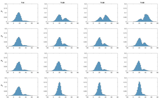
Figure 16. SEnKS approach: Marginal posterior distributions of the initial temperature $f({\mathit{r}}_{0,i}|{\mathit{d}}_{0:T})$ at time $T=0,20,30,50$ at monitoring locations ($i=1,2,3,4$) denoted ($p_1,p_2,p_3,p_4$). The horizontal axes representing temperature are expressed in ${}^{\circ }$C.

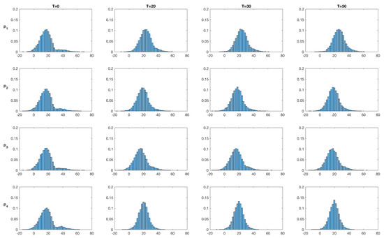
Figure 17. EnKS approach: Marginal posterior distributions of the initial temperature $f({\mathit{r}}_{0,i}|{\mathit{d}}_{0:T})$ at time $T=0,20,30,50$ at monitoring locations ($i=1,2,3,4$) denoted ($p_1,p_2,p_3,p_4$). The horizontal axes representing temperature are expressed in ${}^{\circ }$C.

Figure 18 displays the MMAP predictions of the initial temperature field based on the SEnKS and the traditional EnKS at time $T=0,20,30,50$. For the SEnKS, the high temperature area is clearly identifiable with clear contrast from time $T=30$ while for the EnKS the high temperature area is hardly ever identifiable on the MMAP predictions that show little contrast. Figure 19 displays the MMAP prediction of the initial temperature field at $T=50$ along the section A-A’, see Figure 12, for the SEnKS and the traditional EnKS. The SEnKS clearly identifies the high temperature area and the $80\%$ HDI covers the truth, while the EnKS clearly fails to identify the high temperature area and the $80\%$ HDI does not even cover it.

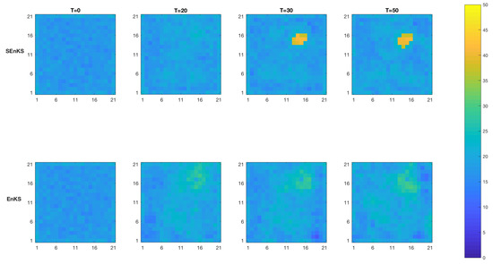
Figure 18. MMAP predictions of the initial temperature (${}^{\circ }$C) field at time $T=0,20,30,50$ for the SEnKS approach (upper) and the EnKS approach (lower).

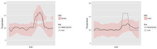
Figure 19. MMAP predictions of the initial temperature (${}^{\circ }$C) field $({\mathit{r}}_0|{\mathit{d}}_{0:T})$ with $80\%$ HDI in cross section A-A’ at time $T=50$ with SEnKS (left) and with EnKS (right).

Realizations of the posterior model at $T=50$ based on the SEnKS and the traditional EnKS algorithms are displayed in Figure 20 and Figure 21, respectively. The SEnKS produces realizations that appear bi-modal while the ensemble members from the EnKS display more symmetric spatial histograms. Even though the differences between the realizations are quite subtle, they are consistent with previous results.

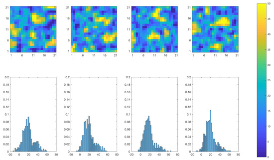
Figure 20. SEnKS approach: Realizations from the posterior distribution $f({\mathit{r}}_0|{\mathit{d}}_{0:T})$ of the initial temperature field at time $T=50$. Upper panels: the colorbar gives the temperature in ${}^{\circ }$C. Lower panels: the horizontal axes represent the temperature (${}^{\circ }$C), the vertical axes represent the relative prevalence of each temperature value for the realization right above.

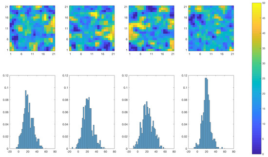
Figure 21. EnKS approach: Realizations from the posterior distribution of the initial temperature field $f({\mathit{r}}_0|{\mathit{d}}_{0:T})$ at time $T=50$. Upper panels: the colorbar gives the temperature in ${}^{\circ }$C. Lower panels: the horizontal axes represent the temperature (${}^{\circ }$C), the vertical axes represent the relative prevalence of each temperature value for the realization right above.

Table 4 shows that RMSE of the MMAP prediction relative to the true initial temperature field for the SEnKS is approximately $20\%$ lower than for the EnKS.

Table 4. RMSE comparing the MMAP prediction of the initial temperature field and the initial temperature field at time $T=50$.

	SEnKS	ENKS
$RMS{E}_{T=50}$	2.92	3.72

This test case clearly illustrates the ability of the SEnKS to conserve multimodality in the posterior distribution, and it leads to predictions with better contrast and accuracy. We conclude that the SEnKS algorithm provides a more reliable reconstruction of the initial state of the temperature field than the traditional EnKS algorithm. Note that the posterior model for the unknown diffusivity field $f(log(\mathit{\lambda })|\mathit{d})$ can also be assessed with the two algorithms. When comparing the MMAP predictions relative to the true diffusivity field, see Figure 12, we observe that none of the algorithms provide reliable predictions. We conclude that the small scale variations in the field are not sufficiently distinct to be identified.

4. Discussion

The traditional EnKF and EnKS algorithms provide an ensemble that directly represents the posterior models $f({\mathit{r}}_{T+1}|{\mathit{d}}_{0:T})$ and $f({\mathit{r}}_{0:T}|{\mathit{d}}_{0:T})$, respectively. Hence, the posterior models can be assessed by displaying statistics based on these ensembles. Reliable assessment of the posterior model in the two test cases can be obtained with approximately 1000 ensemble members. The SEnKF and SEnKS algorithms under study provide an ensemble of the augmented posterior models, $f({\tilde{\mathit{r}}}_{T+1},\mathit{\nu }|{\mathit{d}}_{0:T})$ and $f({\tilde{\mathit{r}}}_{0:T},{\mathit{\nu }}_{0:T}|{\mathit{d}}_{0:T})$, respectively. In order to obtain the posterior models of interest,$f({\mathit{r}}_{T+1}|{\mathit{d}}_{0:T})$ and $f({\mathit{r}}_{0:T}|{\mathit{d}}_{0:T})$, the conditioning on $\mathit{\nu }\in A$ must be made by empirical sampling based inference, see [21,22]. This inference requires the estimation of the expectation vector ${\mathit{\mu }}_{\tilde{r}\nu }$ and covariance matrix ${\Sigma }_{\tilde{r}\nu }$. The two test cases are defined on a $(21\times 21)$-grid for both ${\tilde{\mathit{r}}}_t$ and $\mathit{\nu }$—hence in dimension 882. The expectation and covariance will have 882 and 389,403 unique entries, respectively. Our experience from this study is that approximately 10,000 ensemble members are required to obtain reliable assessment of the posterior models of interest. To reduce the ensemble size, we have tested various localization approaches [29], without notable success, and leave the subject for further research.

5. Conclusions

Data assimilation of spatio-temporal variables with multimodal spatial histograms is challenging. Traditional ensemble Kalman algorithms enforce a regression towards the mean due to the linearized conditioning on observations, hence the multimodality is averaged out. We introduce the selection ensemble Kalman algorithms, termed SEnKF and SEnKS. These algorithms are based on recursive expressions similar to the ones justifying the traditional ensemble Kalman algorithms, but they are defined in an augmented space including the selection variable. From the two case studies, we conclude that multimodality is much better represented by the selection ensemble Kalman algorithms than by the traditional ones. We obtain RMSE reductions in the range of 20 to 30%.

The traditional ensemble Kalman algorithms provide an ensemble representation of the posterior model of interest hence making assessment of the posterior pdf simple. The selection ensemble Kalman algorithms are defined in an augmented space and conditioning on the selection variable must be made a posteriori. For this conditioning to be reliable, the ensemble size needs to be much larger than for the traditional algorithms. Hence, there is a trade-off between improved reproduction of multimodal characteristics of the phenomenon under study and the computational demands. In our case study, the ensemble size needed to be increased by approximately a factor of ten.

We have not fully explored the possibilities of robust estimation of model parameters in the conditioning of the selection variable. This robustification may reduce the ensemble size requirements. Note that parallelization in forwarding of the ensemble is possible and it will reduce the computer demands.

References

- Kalman, R.E. A new approach to linear filtering and prediction problems. Trans. ASME-J. Basic Eng. 1960, 82, 35–45. [Google Scholar] [CrossRef]
- McElhoe, B.A. An Assessment of the Navigation and Course Corrections for a Manned Flyby of Mars or Venus. IEEE Trans. Aerosp. Electron. Syst. 1966, AES-2, 613–623. [Google Scholar] [CrossRef]
- Evensen, G. Sequential data assimilation with a nonlinear quasi-geostrophic model using Monte Carlo methods to forecast error statistics. J. Geophys. Res. 1994, 99, 10143. [Google Scholar] [CrossRef]
- Myrseth, I.; Omre, H. The Ensemble Kalman Filter and Related Filters. In Large Scale Inverse Problems and Quantification of Uncertainty; John Wiley & Sons, Ltd.: London, UK, 2010; chapter 11; pp. 217–246. [Google Scholar]
- Houtekamer, P.L.; Mitchell, H.L.; Pellerin, G.; Buehner, M.; Charron, M.; Spacek, L.; Hansen, B. Atmospheric Data Assimilation with an Ensemble Kalman Filter: Results with Real Observations. Mon. Weather. Rev. 2005, 133, 604–620. [Google Scholar] [CrossRef]
- Sakov, P.; Oliver, D.; Bertino, L. An Iterative EnKF for Strongly Nonlinear Systems. Mon. Weather. Rev. 2012, 140, 1988–2004. [Google Scholar] [CrossRef]
- Sklar, A. Random variables, joint distribution functions, and copulas. Kybernetika 1973, 9, 449–460. [Google Scholar]
- Isaaks, E.H.; Srivastava, R.M. Applied Geostatistics; Oxford University Press: New York, NY, USA, 1989. [Google Scholar]
- Bertino, L.; Evensen, G.; Wackernagel, H. Sequential Data Assimilation Techniques in Oceanography. Int. Stat. Rev. 2003, 71, 223–241. [Google Scholar] [CrossRef]
- Simon, E.; Bertino, L. Application of the Gaussian anamorphosis to assimilation in a 3D coupled physical-ecosystem model of the North Atlantic with the EnKF: A twin experiment. Ocean. Sci. 2009, 5, 495–510. [Google Scholar] [CrossRef]
- Xu, T.; Gomez-Hernandez, J. Characterization of non-Gaussian conductivities and porosities with hydraulic heads, solute concentrations, and water temperatures. Water Resour. Res. 2016, 52, 6111–6136. [Google Scholar] [CrossRef]
- Gu, Y.; Oliver, D. An Iterative Ensemble Kalman Filter for Multiphase Fluid Flow Data Assimilation. SPE J. 2007, 12, 438–446. [Google Scholar] [CrossRef]
- Evensen, G. Analysis of iterative ensemble smoothers for solving inverse problems. Comput. Geosci. 2018, 22, 885–908. [Google Scholar] [CrossRef]
- Dovera, L.; Della Rossa, E. Multimodal ensemble Kalman filtering using Gaussian mixture models. Comput. Geosci. 2010, 15, 307–323. [Google Scholar] [CrossRef]
- Rimstad, K.; Omre, H. Approximate posterior distributions for convolutional two-level hidden Markov models. Comput. Stat. Data Anal. 2013, 58, 187–200. [Google Scholar] [CrossRef]
- Grana, D.; Fjeldstad, T.; Omre, H. Bayesian Gaussian Mixture Linear Inversion for Geophysical Inverse Problems. Math. Geosci. 2017, 49, 493–515. [Google Scholar] [CrossRef]
- Besag, J. Spatial interaction and the statistical analysis of lattice systems. J. R. Stat. Soc. Ser. 1974, 36, 192–236. [Google Scholar] [CrossRef]
- Le Loc’h, G.; Beucher, H.; Galli, A.; Doligez, B. Improvement In The Truncated Gaussian Method: Combining Several Gaussian Functions. In Proceedings of the ECMOR IV—4th European Conference on the Mathematics of Oil Recovery; European Association of Geoscientists & Engineers: Røros, Norway, 1994. [Google Scholar] [CrossRef]
- Oliver, D.; Chen, Y. Data Assimilation in Truncated Plurigaussian Models: Impact of the Truncation Map. Math. Geosci. 2018, 50, 867–893. [Google Scholar] [CrossRef]
- Arellano-Valle, R.B.; Branco, M.D.; Genton, M.G. A unified view on skewed distributions arising from selections. Can. J. Stat. 2006, 34, 581–601. [Google Scholar] [CrossRef]
- Omre, H.; Rimstad, K. Bayesian Spatial Inversion and Conjugate Selection Gaussian Prior Models. arXiv 2018, arXiv:1812.01882. [Google Scholar]
- Conjard, M.; Omre, H. Spatio-temporal Inversion using the Selection Kalman Model. arXiv 2020, arXiv:stat.ME/2006.14343. [Google Scholar]
- Cappé, O.; Moulines, E.; Ryden, T. Inference in Hidden Markov Models (Springer Series in Statistics); Springer-Verlag: Berlin/Heidelberg, Germany, 2005. [Google Scholar]
- Moja, S.; Asfaw, Z.; Omre, H. Bayesian Inversion in Hidden Markov Models with Varying Marginal Proportions. Math. Geosci. 2018, 51, 463–484. [Google Scholar] [CrossRef]
- Evensen, G. Data Assimilation; Springer-Verlag: Berlin Heidelberg, Germany, 2006; Volume 307. [Google Scholar] [CrossRef]
- Evensen, G. The Ensemble Kalman filter: Theoretical Formulation and Practical Implementation. Ocean. Dyn. 2003, 53, 343–367. [Google Scholar] [CrossRef]
- Burgers, G.; Van Leeuwen, P.J. On the Analysis Scheme in the Ensemble Kalman Filter. Mon. Weather. Rev. 1998, 126, 1719–1724. [Google Scholar] [CrossRef]
- Hyndman, R. Computing and Graphing Highest Density Regions. Am. Stat. 1996, 50, 120–126. [Google Scholar]
- Gaspari, G.; Cohn, S. Quarterly Journal of the Royal Meteorological Society. J. Comput. Graph. Stat. 1999, 125, 723–757. [Google Scholar]
© 2020 by the authors. Licensee MDPI, Basel, Switzerland. This article is an open access article distributed under the terms and conditions of the Creative Commons Attribution (CC BY) license (http://creativecommons.org/licenses/by/4.0/).