1. Introduction
Dual-arm robotic systems are widely used in various settings to expand the working range compared with single-arm robotic systems. As described in [
1,
2], dual-arm systems are widely used in space robots and disaster environments. To perform complicated tasks, each arm is provided with different targets and trajectories. One of the challenges in dual-arm cooperation control is to avoid self-collisions, which dramatically constrain the working range and affect the continuous motion of each arm. In this paper, we propose a self-collision avoidance method, where a dual-arm robot has the ability to detect and avoid self-collisions, to deal with such problems.
For self-collision avoidance methods, the collision model is critical. In collision models, a model of the robot is approximated, and relative position information is obtained between the robot links. In a collision model, the distance between the two arms is calculated in real time. A function related to the minimum distance is used to prevent robot collisions.
A collision model is always formed by various convex hulls. In previous studies, a collision detection model was built using a large number of polygons [
3,
4]. To tightly fit the different volumes of the robot, researchers have developed algorithms to build each convex polyhedral model. Examples include the tight-fitting oriented bounding box trees (OBB) algorithm [
5], and the axis-aligned bounding boxes (AABB) algorithm [
6]. Many algorithms have been proposed to calculate the distance in convex polyhedral models such as the fast and robust polyhedral collision detection (V-Clip) algorithm [
7]. As the features of polyhedral-based collision model are vertices, edges, and faces [
8], the computational cost to determine if a pair of polyhedrons are disjointed and to compute the distance between them is high [
7]. To reduce the computational cost between different collision models, researchers have developed sphere-based collision models to replace polygon-based collision models [
9,
10,
11]. In [
9,
10], a sphere-based collision model was built using a sweep sphere model. For the sweep sphere line, the distance between two sweep sphere lines is calculated. The minimum distance may have a discontinuous gradient when the pair of closest points is on the two shapes [
11]. In [
11], an improved method was proposed, where a collision model was built using finite discretized spheres with the same radius. Compared with the sweep sphere model, the finite discretized sphere collision model algorithm [
11] only needs to measure the distance between the center of each sphere (all possible distances between different spheres), which has a low computational cost. However, due to the difference in the links for each arm, the model of the origin robot may not be able to be approximated using spheres with the same radius.
Self-collision avoidance methods can be divided into two categories: (i) on-line (real-time) self-collision avoidance [
3,
6,
12,
13,
14,
15] and (ii) off-line planning of a collision-free trajectory [
9,
16,
17] for the robot. Real-time self-collision avoidance methods always rely on the minimum distance between collision pairs. Earlier researchers proposed a collision model to check a collision pair in real time, where the robot abruptly stops when the collision model predicts a collision [
4,
6]. However, this behavior may influence the stability of the robot. To improve the results, researchers have proposed the skeleton algorithm [
13,
18,
19,
20], which establishes an artificial repulsive potential field to generate the virtual repulsive force on the robot links. Meanwhile, the skeleton algorithm has already been applied on the The German Aerospace Center(DLR) humanoid manipulator Justin [
13]. Based on the dynamic model of the robot, the robot can generate a smooth trajectory to avoid self-collision. Although these algorithms can achieve self-collision avoidance, they do not consider the performance of the arm end-effector. Compared to these traditional methods, some researchers have proposed a unified framework for detecting collisions in real time by using a series of sensors capable of estimating the joint torque and acceleration [
14]. However, using sensors always increases the cost of the robot due to the more expensive hardware.
In off-line methods, a collision-free trajectory is planned in advance. Based on the rapidly-exploring random tree (RRT) [
21] algorithm, researchers have proposed an algorithm to plan a collision-free path [
22] for each arm in advance. The extended stochastic trajectory optimization for motion planning (STOMP) algorithm, which is an improvement of the STOMP [
23] algorithm, obtains a qualitatively collision-free trajectory according to user preferences [
24]. Some researchers have presented a method for generating and synchronizing path-constrained trajectories for multi-robot systems [
25]. Regarding the Asea Brown Boveri (ABB) company, they proposed a method to monitor the multi-arm, whether local at the collision space at the same time [
26], before planning the path of each arm. With the development of machine learning, researchers can set different collision regions using efficient data-driven techniques to predict the joint collision position based on a support vector machine (SVM) algorithm [
16,
17], which may lead to higher computational costs. In particular, the method proposed in [
16] has already been applied on the Istituto Italiano di Tecnologia (IIT) SCAFoI humanoid robot. Compared with on-line methods, off-line planning can be dangerous. For example, a robot can be misguided in planning a collision trajectory. In off-line planning, the collision-free trajectory must be planned before the arm moves to the target, so off-line planning also leads to higher computational costs.
In this paper, we propose an optimized collision model that decreases the computational cost as well as the robot hardware cost. In addition, it increases the reaction speed and accuracy simultaneously without any sensors to detect the relative distance of the two arms. To demonstrate the validity of the algorithm, two independent arms with conflicting tasks are considered, so that each arm is in danger of self-collision. The goal of this study is to develop a real-time self-collision avoidance method that consists of: (1) a collision model based on a finite number of spheres with different radii; and (2) a suitable self-collision avoidance strategy. The main contributions of this study are summarized as follows:
- (1)
In this study, we developed a collision model by using multiple discretized spherical bounding volumes with different radii, which has fewer spheres and can enclose the robot with a low approximation error.
- (2)
To calculate all possible distances between spheres with different radii, a sensitivity index was proposed to measure the distance between different spheres. According to the minimal sensitivity index, the magnitude of the repulsive velocity can be measured using the sigmoid function.
- (3)
The repulsive velocity will generate on each control point of each link. Based on the kinematic model of each arm, the repulsive velocity on each control point is projected in the velocity direction of the end-effector, which helps the robot modify the magnitude of the end-effector velocity, while generating the repulsive velocity on the control points to avoid self-collision at the collision spheres.
The remainder of this paper has the following structure. In
Section 2, the collision model of the dual-arm robot is developed, along with the method for calculating the minimum distance between the sphere bounding volumes.
Section 3 describes the development of the real-time self-collision avoidance strategy of the robot. The repulsive velocity acts on the center of the spherical volumes to generate a smooth trajectory to avoid self-collision. In
Section 4, the modeling parameters are identified in an example in which a robot is used. Simulations and experiments demonstrate the validity of the proposed algorithm.
Section 5 concludes this work.
3. Self-Collision Avoidance Strategy
Our self-collision avoidance strategy relies on relationships between the minimal sensitivity index, the repulsive velocity, and the angular velocity of the arm.
Section 3.1 illustrates the relationship between the minimal sensitivity index and the repulsive velocity, which shows how to use the repulsive velocity according to the minimal sensitivity index.
Section 3.2 illustrates the relationship between the repulsive velocity and the velocity at the end-effector of each arm.
Section 3.3 shows that to solve self-collision using our algorithm, each arm must be controlled at the joint velocity level.
3.1. Repulsive Velocity between Two Spheres
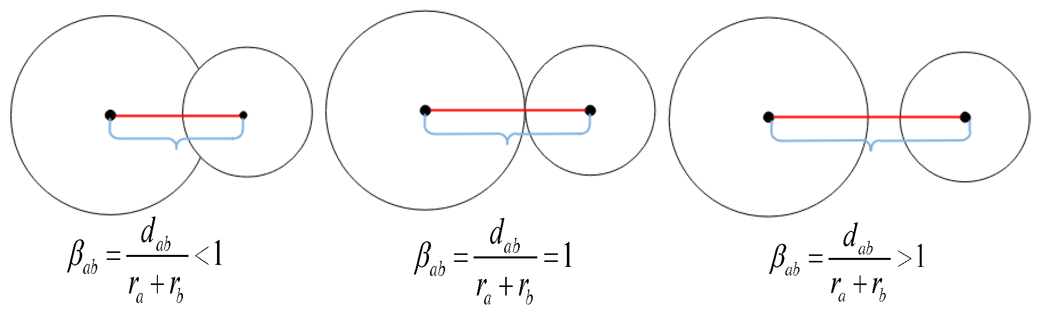
Each arm of the robot has multiple bounding volumes, and the minimal sensitivity index indicates the relationship between the closest bounding volumes. When , the repulsive velocity is produced at these control points.
Meanwhile, inspired by the on-line method of human–robot collision avoidance algorithms in [
27], we chose the sigmoid function to measure the magnitude of the repulsive velocity. By using the sigmoid function, the magnitude of the repulsive velocity
can be calculated as
where Vmax is the maximum velocity allowed at the end of the robot and
is the shape factor, as described in [
27]. If Vmax = 0.25 and
, the profile shown in
Figure 5a is achieved, which illustrates the relationship between the minimal sensitivity index and the repulsive velocity.
From the profile shown in
Figure 5, the sigmoid function not only ensures the continuity of the speed change, but when the relative distance of the arm becomes smaller, the gradient of the repulsive change continues to be changed. In particular, in
Figure 5, a shorter
resulted in a larger repulsive velocity, helping the robot avoid self-collision. Meanwhile, we can conclude that when
, the magnitude of the repulsive velocity
= 0.25 is equal to the maximum velocity
Vmax of the end-effector. This can also define the radii of each sphere.
Considering each link of the robot as the cylinder and the radius of each cylinder (link) is , the radius of each sphere can be defined according to . In this way, we can define the radius of each sphere. When , it indicates a collision between the arms; when the magnitude of the repulsive velocity , it indicates that the robot will stop motion.
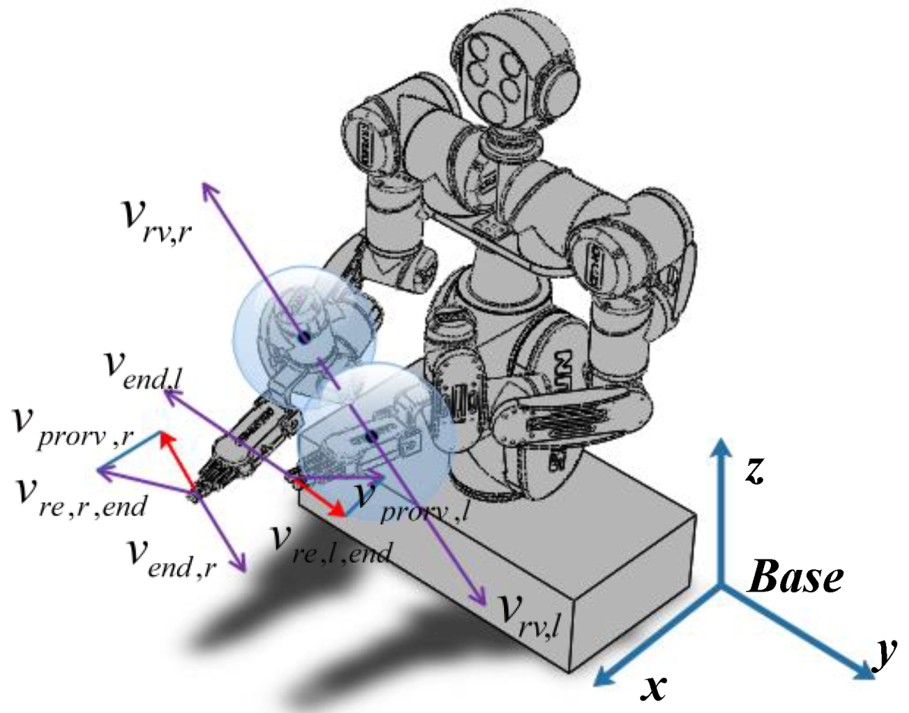
As illustrated in
Figure 5b, the position of the control point
a, on the left, is defined as
, which is expressed in the base frame, and the other point
b, on the right, is
. Then, the repulsive velocity direction can be defined as
The repulsive velocity produced at the control points can be computed as:
Section 3.1 introduced the calculation of the repulsive velocity between two spheres. In reality, the strategy must be applied on the dual-arm system in 3D space.
Our approach is illustrated on the dual-arm robot in
Figure 6, which has a left arm (
l) and a right arm (
r). Each arm has a different original velocity on the end-effector, which is defined as
, where
k = l or
r represents the left or right arm. The original joint velocity is defined as
, where
i represents the
i-th joint of each arm. Thus, the joint velocities
can be calculated as follows:
where
are the Jacobian matrices with respect to the end-effector of the robotic arms, and
is the pseudo-inverse;
and
represent the linear and angular velocity of the end–effector of each arm, respectively.
3.2. Repulsive Velocity at the End-Effector
As illustrated in
Figure 6, a bounding sphere is centered at point of the left arm and at point
b of the right arm of the robot. These control points both have repulsive velocity
(
k = l or
r) when
, which implies that these spherical bounding volumes will collide. The repulsive velocity acts on the centers of the spheres, as discussed in
Section 2.
The repulsive velocity needs to be controlled at the joint velocity level. To determine the repulsive velocity of the control point, only the joints prior to this control point should be given a repulsive joint velocity. In the case shown in
Figure 6, the repulsive joint velocity is generated on joints 1–5 of the left arm, and on joints 1–7 of the right arm.
Defining part of the repulsive joint velocity of the
k arm from joint 1 to joint
i (
i ≤
j) as
(
k =
l or
r) of the arm, the repulsive joint velocity of this part of the arm can be calculated as follows:
where
are Jacobian matrices for the control points, as illustrated in
Figure 2a in arm
k (
k = l or
r). Here, only the positions of the two control points are controlled, so we set
in arm
k (
k = l or
r).
The velocity of the joints after/distal to the control point was set to zero. In this way, the repulsive joint velocity
(
k = l or
r) can be obtained as
According to the repulsive joint velocity, the end-effector velocity of the arm is generated with an end-effector repulsive velocity
as
Due to the collision model, which was built using discretized spheres with different radii and detecting the minimum distance between the spheres, the minimum distance points could change instantaneously, causing discontinuous velocities and non-smoothness in the overall behavior of the system. In this way, we chose to project the velocity in the direction of the end-effector velocity, which only changes the magnitude of the end-effector velocity, to alleviate this situation. Meanwhile, this strategy can also generate the repulsive velocity.
3.3. Real-Time Self-Collision Avoidance
As illustrated above, the end-effector repulsive velocity calculated by (14) can have different directions from the original end-effector velocity (k = l or r), which is planned in advance for a dual-arm task. The end-effector repulsive velocity can drive the effector to an uncertain direction, and the desired task may not be finished. To solve this problem, the algorithm modifies only the magnitude of the original end-effector velocity and keeps the direction unchanged.
Using the end repulsive velocity
calculated in (14), the end-effector repulsive velocity
(
k = l or
r) is then projected to the original velocity of the end-effector
(
k = l or
r), which is represented by the red lines in
Figure 6.
The angle
γk between
and
(
k = l or
r) and can be calculated as
The projected repulsive velocity
(
k = l or
r) can be calculated as
Summing the projected repulsive velocity
and the original end-effector velocity
, the new velocity of the end-effector
(
k = l or
r) is obtained as
Next, the new joint velocity can be calculated using (18), where
(
k =
l or
r) are the new joint velocities:
4. Simulation and Application of the Algorithm
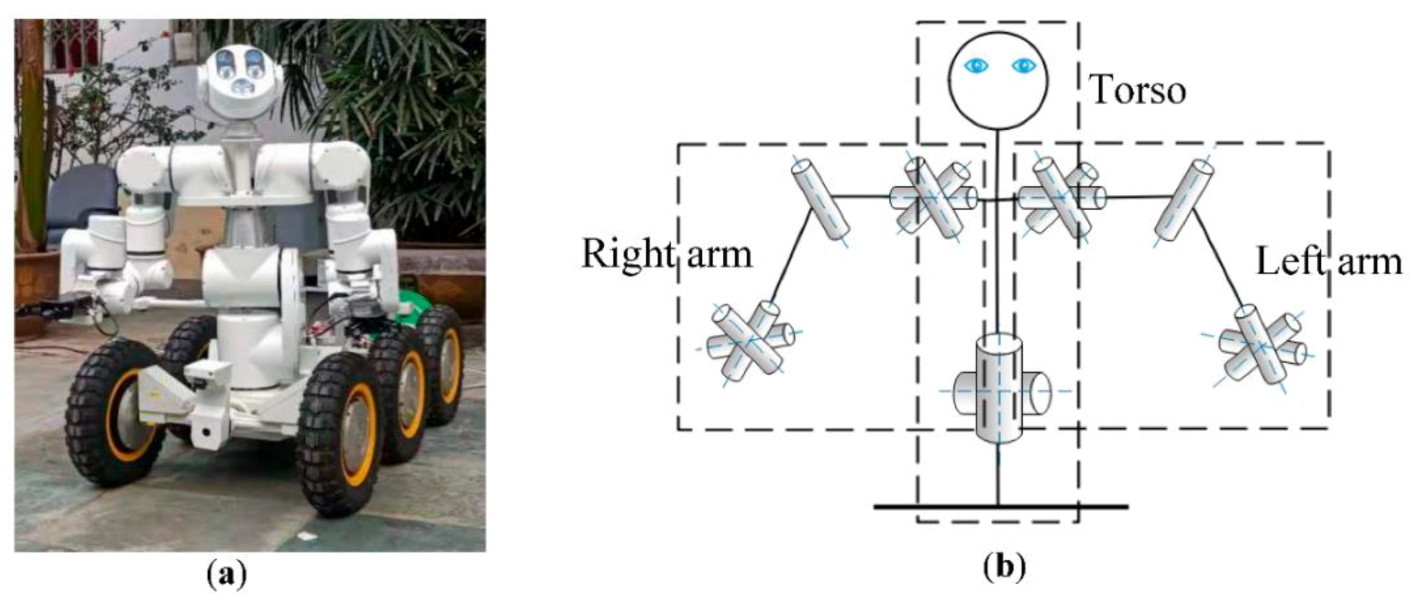
This section presents the simulation and experiment for self-collision avoidance by a robot using the proposed algorithm. The robot has dual 7-DOF arms, as shown in
Figure 1. To avoid collision of the links with one arm, the joints were set as indicated in
Table 1. According to the specifications of the robot, the maximum velocity of the end-effect was below 2.5 m/s.
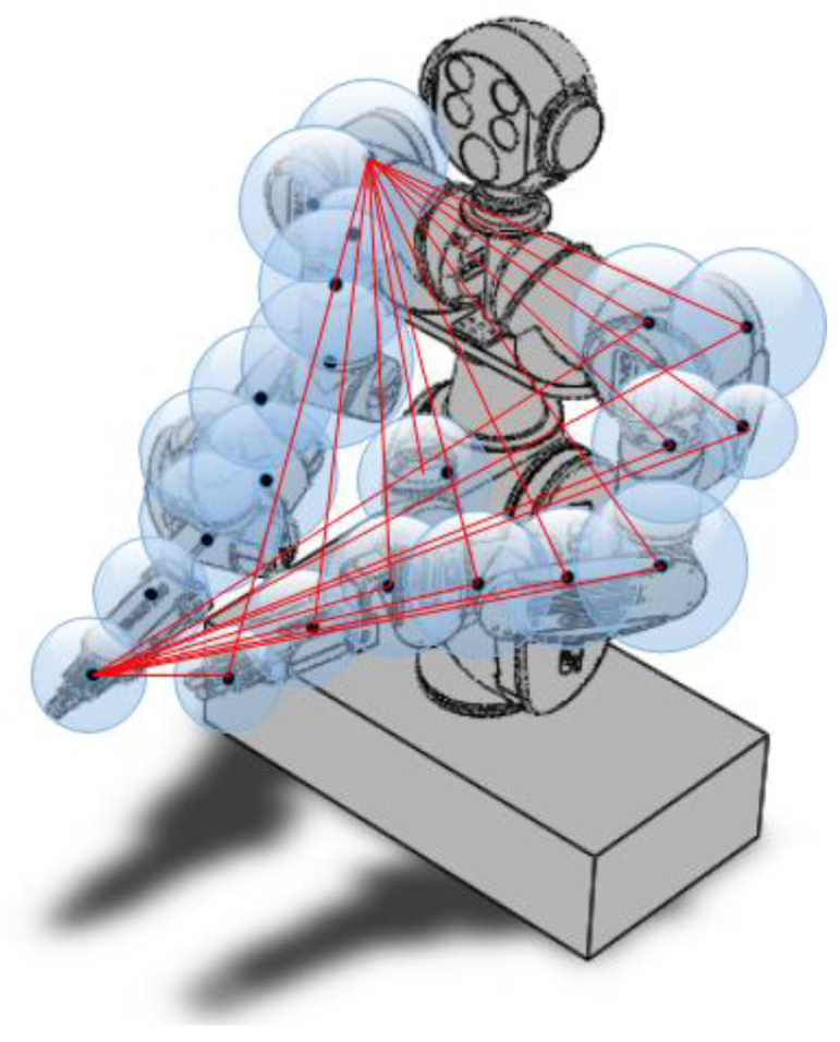
The collision model was constructed with 10 spheres centered at 10 control points on each arm, as illustrated in
Figure 7. The red lines in
Figure 7 represent the distances between the control points on different arms. The diameters of the spheres are listed in
Table 2.
As the collision model is built, the sensitivity index
βlr is calculated according to
Section 2. The new joint velocities
(
k =
l or
r) are then calculated for self-collision avoidance when one spherical volume collides with another spherical volume.
4.1. Simulations
The simulation was performed using an Intel Atom
® E3845 processor (Quad Core, 1.91 GHz, 10 W) with 32 GB of RAM, and Ubuntu 16.04 using ROS Kinetic. The simulation results are shown in
Figure 8.
The algorithm was simulated on a dual-arm robot with 10 control points on each arm. First, the system needs to detect and update the matrix in real time. Following the steps presented in
Section 3, the new joint velocities were calculated, which changes the motion of the robot to avoid collision. These processes are illustrated in
Figure 8.
In
Figure 8(a.i, i = 1, 2), we intentionally set the same target positions for the two arms (i.e., without the self-collision avoidance algorithm, the two arms will collide as the end-effectors approach their targets). Actually, with the self-collision avoidance strategy, the repulsive velocities are calculated on the control points. In
Figure 8(a.1), the repulsive velocity acted on the end-effector of the left arm and link 6 of the right arm; in
Figure 8(a.2), the repulsive velocity acted on the end-effectors of the robotic arms. Both the left and right arms changed their motion to avoid collision. The repulsive velocity on each arm both act on the end-effectors, which makes each arm move away from their target.
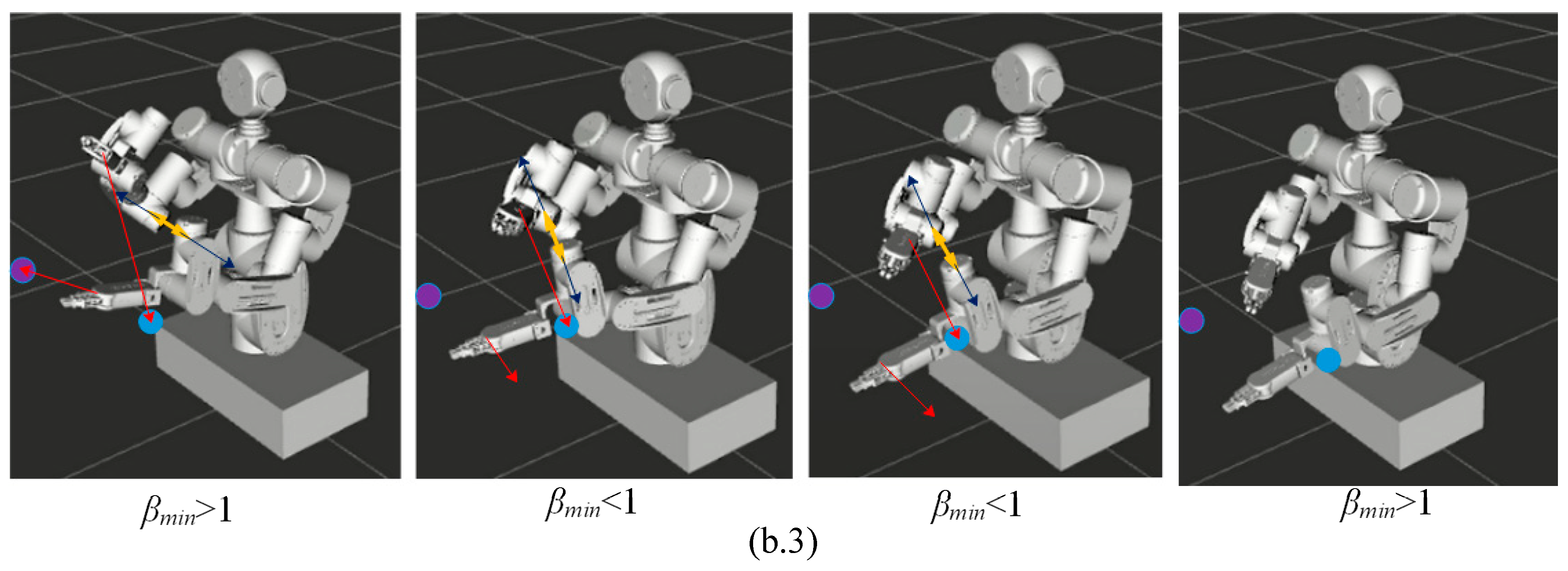
In
Figure 8(b.i, i = 1, 2, 3), we intentionally set the left and right end-effectors with different targets. Without the self-collision avoidance algorithm, the two arms will collide as the end-effectors approach their targets. With the self-collision avoidance strategy, the repulsive velocities were calculated on the control points. In
Figure 8(b.1), the repulsive velocity acted on link 7 of the left arm and link 6 of the right arm; in
Figure 8(b.2) the repulsive velocity acted on the end-effector of the left arm and link 6 of the right arm; in
Figure 8(b.3) the repulsive velocity acted on link 6 of the left arm and link 6 of the right arm. The simulated process of avoiding self-collision is illustrated in
Figure 8(b.i, i = 1, 2, 3). The right arm and left arm both changed their trajectories to avoid self-collision, but one of the dual-arms was also close to the target in the other trajectory. In
Figure 8(b.1), the left arm was close to the target. In
Figure 8(b.2), the left arm was close to the target. In
Figure 8(b.3), the right arm was close to the target.
A common approach for self-collision avoidance is the artificial potential field in which one of the arms is modeled with an obstacle. However, these strategies often result in a (topologically unnecessary) minimum [
28]. Meanwhile, we completed two simulations using the traditional artificial potential field method. These methods do not consider the velocity vector of the end-effector. In
Figure 9a, two arms of dual-arm had a common target and in
Figure 10a, two arms of dual-arm had different targets. The trajectories of each arm illustrated that the two arms both easily fell into the local minimum and vibrated around the local minimum points, as illustrated in
Figure 9b,
Figure 10b, respectively.
Compared with the traditional artificial potential field method, the method of this paper improved the problems of the traditional method due as we considered the action of the end-effector. Meanwhile, the simulation results of the different tasks described above prove the effectiveness of this real-time self-collision algorithm based on the kinematic model of a robot. The algorithm uses a simple collision model and the distance calculation method to decrease the computational costs of the algorithm.
4.2. Experimental Results
The algorithm was implemented on a dual-arm robot in an office environment, and demonstrated the change of the end-effector velocity. The sampling frequency of the control loop was set at 50 Hz.
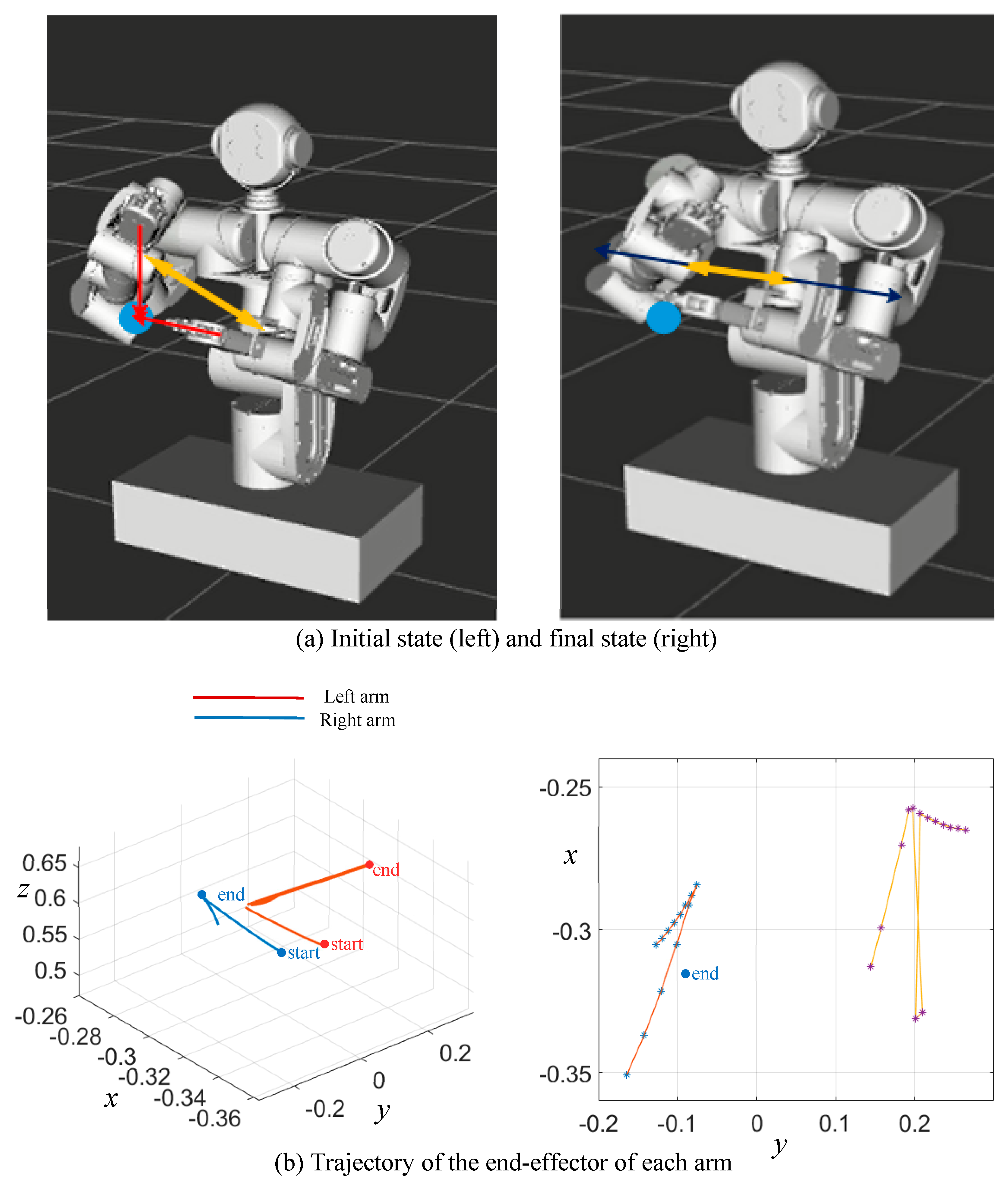
Figure 9 and
Figure 10 show the results of the two tasks. In
Figure 9, the two arms of the dual-arm robot had a common target, while in
Figure 10, each arm had a different target.
Figure 11a shows the snapshots of the experiment. The velocity profile and the trajectory of the end-effect of the arms are shown in
Figure 11b,c, respectively. As the two arms had the same target, both arms changed trajectory to avoid self-collision. In fact, both arms moved away from the target.
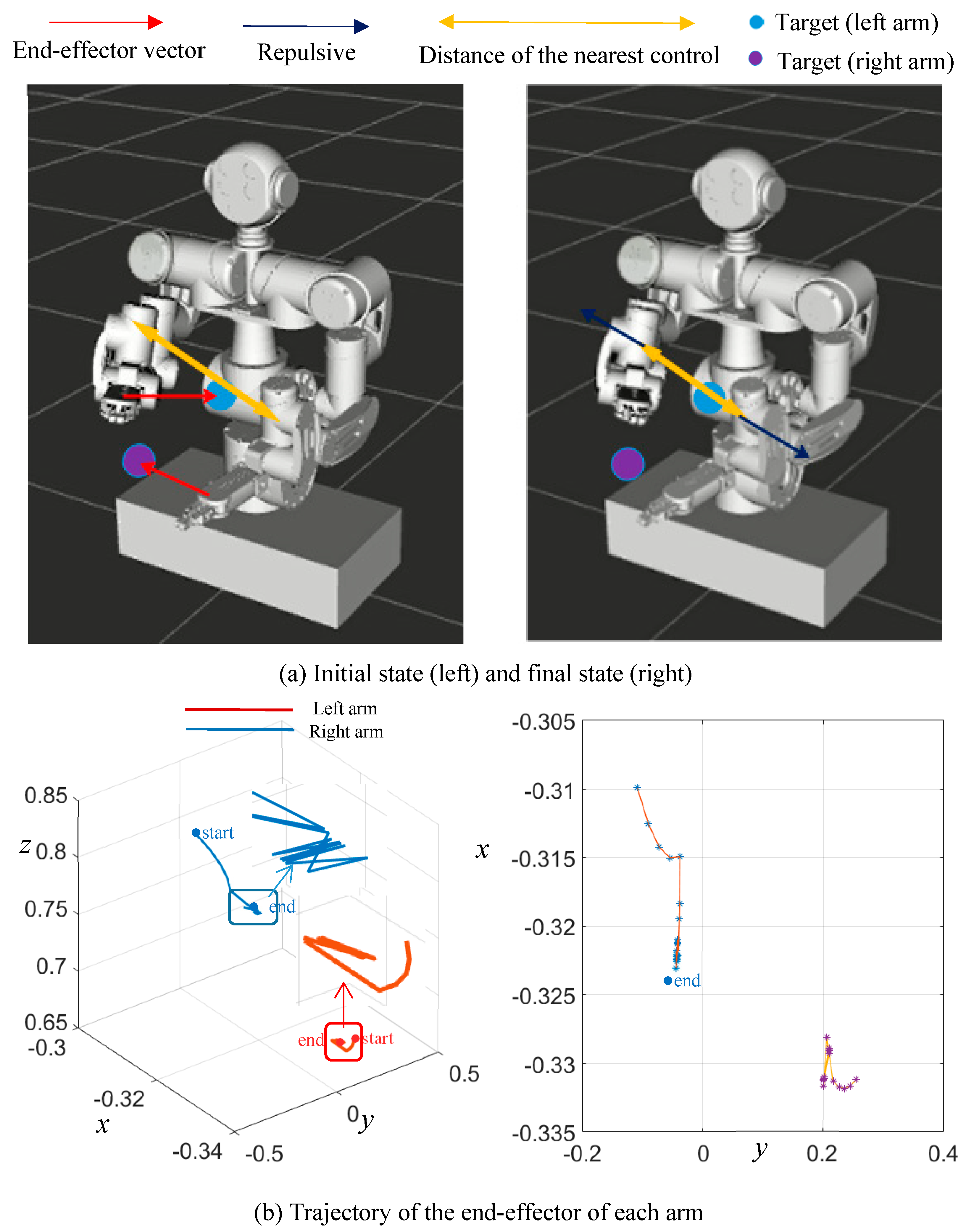
In the second experiment, the robotic arms had different targets, as illustrated in
Figure 12a. The velocity profile of the end-effector and the trajectories of the two arms are shown in
Figure 12b,c, respectively.
As the two arms had different targets, each arm changed its motion to find a collision-free trajectory. As illustrated in
Figure 12, the repulsive velocity produced the end-effect on the left arm and acted on link 6 of the right arm. In this way, the repulsive velocity was projected onto the end-effect of the left arm. In other words, both arms in the dual-arm system changed their motion to avoid self-collision: the right arm changed its motion to approach the target, whereas the left arm changed its motion by moving away from the target and the right arm.
Meanwhile, as illustrated in
Figure 11b,
Figure 12b, respectively, although there were fluctuations in the end-effector velocity, the fluctuation did not affect the results of the experiment.
These experiments were similar to the simulations, which are described in
Section 4.1, and demonstrated the effectiveness of our algorithm in simulation A (robotic arms with the same target) and simulation B (robotic arms with different targets). Meanwhile, these demo of the experiments were upload on the web as illustrate in
Supplementary Materials).


