Optical Fibres for Condition Monitoring of Railway Infrastructure—Encouraging Data Source or Errant Effort?

Abstract

The condition of railway infrastructure is currently assessed by track recording cars, wayside equipment, onboard monitoring techniques and visual inspections. These data sources deliver valuable information for infrastructure managers on the asset’s condition but are mostly carried out in time-based intervals. This paper examines the potential of fibre optic cables, which are already installed in cable troughs alongside railway tracks, to monitor railway infrastructure conditions. The sensing technique, known as distributed acoustic/vibration sensing (DAS/DVS), relies on the effect of Rayleigh scattering and transforms the optical fibre into an array of “virtual microphones” in the thousands. This sensing method has the ability to be used over long distances and thus provide information about the events taking place in the proximity of the monitored asset in real-time. This study outlines the potential of DAS for the identification of different track conditions and isolated track defects. The results are linked to asset data of the infrastructure manager to identify the root cause of the detected signal anomalies and pattern. A methodology such as this allows for condition-based and component-specific maintenance planning and execution and avoids the installation of additional sensors. DAS can pave the way toward a permanent and holistic assessment of railway tracks.

1. Introduction

Railway infrastructure is subject to wear and tear. An increasing traffic volume, higher train speeds and thus burgeoning loads enhance the deterioration of infrastructure and challenge infrastructure managers (IM) today in their task of ensuring the required track quality and availability. The latter two are essentially determined by both the condition of the rolling stock and railway infrastructure. While the rolling stock condition lies in the responsibility of railway undertakings (RU), infrastructure managers have the duty of caring for the condition and consequently the availability of railway tracks. The deterioration of, e.g., the ballast and track geometry, as a consequence of the operated trains and their traffic load thus results in maintenance demands that are by no means negligible for keeping track quality at a required standard.

A good track quality enables trains to operate at higher speeds and thus increases the capacity (number of operated trains) and track availability. In addition, a well-maintained track improves the safety of railway operations and reduces the risk of accidents. However, an increasing traffic volume leads to higher track possession and shortened track closures for maintenance and consequently fewer time slots available for maintenance. Having said this, it is also clear that more traffic and consequently higher loads lead to higher maintenance and renewal demands and result in track closures for essential maintenance activities such as tamping or grinding. Therefore, the evaluation and assessment of a railway track is a decisive task for infrastructure managers, and it is becoming even more important to implement a sustainable and condition-based maintenance strategy based on life cycle cost considerations. The evaluation and assessment of a railway track are vital tasks providing essential information to any railway infrastructure manager. Knowledge about track conditions and the ability to distinguish the specific component responsible for the end of service life forms the basis for all sustainable decision making in this context (life cycle management) [1]. Such a strategy can only be effectively implemented when frequent track measurements are carried out since these are the key to data quality and quantity.

Either way, for the assessment of railway tracks and rolling stocks, infrastructure managers have access to several data sources providing them with information on the track and rolling stock conditions with varying degrees of data quality and quantity. Condition monitoring and measuring of both the infrastructure and rolling stock can be classified into four groups: (1) vehicle measures infrastructure; (2) vehicle measures vehicle; (3) infrastructure measures infrastructure and (4) infrastructure measures vehicle.

Track recording cars (TRCs) are commonly used, primarily for measuring the track geometry of the entire network by almost every infrastructure manager. The measurement data from TRCs are well-known, reliable and state-of-the-art, but are by no means a modern concept. These vehicles do not observe the network continuously, which means the local measurements over a specific distance only take place on a now and then basis. These measurement intervals are adequate of course, for sections deteriorating at a moderate pace, but may be too long for critical sections including isolated track defects (white spots), hollow layers (hanging sleepers), subgrade lowering, (insulated) rail joints or even broken rails. Furthermore, measurements from TRCs are not capable of condition monitoring (CM) for turnouts and bridges in particular. These assets are assessed mainly by visual inspection executed by dedicated experts in cyclic intervals every few weeks. Current developments aim beyond a pure track geometry observation as several additional measuring systems are equipped on vehicles for detection of, e.g., rail and catenary profiles or tunnel clearance measurements [2]. A method for increasing the measurement frequency to assess the condition of tracks provides sensors mounted on in-service vehicles/trains (onboard monitoring (OBM)), including axle box accelerometers [3,4] or bogie movement measurements [5,6,7]. These data could be a valuable data source for critical assets and sections and have been examined for almost 20 years. Nevertheless, measurements on a broad scale are still not available and many measurement campaigns struggle to deliver reliable data, resulting in them not yet being proven. These systems are assigned to the first group “vehicle measures infrastructure”. The latter discussed systems aim not only to deliver data on the track condition, but also to assess the health status of vehicle components. Such systems can be classified into the second group, “vehicle measures vehicle”.

In recent years, the application of sensors on turnouts [8] and bridges [9] has been thoroughly investigated. These approaches are very useful to gain knowledge about the condition and behaviour of these assets but deliver only information about specific turnouts or bridges at one location. Furthermore, gaining knowledge on the health status of these assets is becoming more and more decisive as experienced experts—know-how owners with long-term manual inspection experience—retire from service and their valuable knowledge is lost with them. Manual inspections are highly subjective procedures, they are not to be regarded as reproducible and are naturally time-consuming and costly. Some of the aspects of this call to equip thousands of turnouts and bridges with sensors and measures on this scale are scarcely affordable for any IM. Sensors mounted on assets of interest are assigned to the third group, “infrastructure measures infrastructure”.

Lastly, another noteworthy data source that IMs rely on is wayside train monitoring systems (WTMS): “infrastructure measures vehicle”. The main field of application is, accordingly, the monitoring and assessment of rolling stock conditions. WTMS have been gradually expanded and provide additional information about the infrastructure-damaging conditions of vehicles such as dragging equipment or whether vehicles comply with the clearance profile [10,11]. Trackside sensors for rolling stock observations have been used for a long time, are proven systems and monitor the condition of each train passing at the location where they are deployed. Nonetheless, these are local measurements at specific points installed at neuralgic points within the network. The effective extent of the measurement system is determined by the quantity of equipment in use and inevitable gaps can lead to some undetected failures and incidents.

All the above-noted systems have strengths and shortcomings. However, an IM’s strategy and budgetary situation determine the number of installed WTMS. On the one hand, wayside condition monitoring sensors are very costly and hence it is not possible to install them every few kilometres. On the other hand, each sensor equipped for tracking requirements must be maintained from time to time and, in cases of track maintenance, they may have to be removed to prevent sensor damage. The removal of such equipment is not only time-consuming, it also influences the maintained section length in a specific track closure. Permanent measurements, such as axle counters, provide extensive information about vehicle performance at any point in time for each train crossing, but only do so at fixed positions, where measuring equipment of this kind is installed. In contrast, continuous measurements such as track recording cars deliver information at one point in time but do so only for a specific longitude. As a result, there is a lack of data, measurement and information about the track condition. Based on the evaluation methods discussed, the question arises whether there are further data sources without the requirement of additional sensor installations and track closures for measurements.

This paper examines the potential of optical fibres for the monitoring of railway infrastructure conditions that have already been installed alongside railway tracks. A sensing technique named distributed fibre optic sensing (DFOS) is used for the continuous and permanent monitoring of railway tracks from the cable duct whereby two distributed acoustic sensing (DAS) interrogator units were applied to detect all events taking place on or in the proximity of the monitored route. In order to not affect the day to day railway operations, no modifications regarding the fibre layout were made. The systems should prove its ability under realistic boundary conditions to detect potential track failures and isolated track defects. In contrast to new measuring systems, which are developed and installed especially for their respective requirements, in this case, already installed optical fibres are used for monitoring. Such optical fibres were originally installed for signalling and telecommunications and are therefore not actually intended for measurement purposes. The aim of this paper is to investigate whether the condition of the railway infrastructure can be monitored without additional trackside measuring equipment and consequently the number of sensors in the track does not increase. Thus, the focus is clearly on the addition of information about the track that can be generated with existing fibre optic infrastructure and not on the development of the measurement system.

2. Optical Fibres—A Brief Overview

The rise of distributed fibre optic sensing (DFOS) is closely linked to the invention and development of lasers in 1960 [12]. It was also at that time when the possibility to transfer information through an optical fibre carried by a light wave (laser pulse) was detected. Due to high fibre losses, however, only limited transport distances could be realized. A major breakthrough was achieved by Kao and Hockham [13] who demonstrated that high losses in optical fibres occur due to fibre impurities resulting from the production process. This led to intensive activities aimed at removing these impurities, resulting in optical fibres with losses of 20 dB/km in 1970 [14]. Since then, fibre optic sensing has become a major technology, especially in a discipline known as structural health monitoring (SHM), which aims to monitor and determine the structure of large infrastructures (e.g., bridges and tunnels), oil and gas pipelines, vehicles and biomedical devices. Fibre optic sensors can be classified, based on the number of sensors or rather their spatial resolution, into three groups: (1) point sensors; (2) quasi-distributed sensors and (3) distributed sensors [15].

While point sensors are only rarely used, the latter two have found valuable applications in railways. Quasi-distributed sensors are mainly represented by fibre Bragg grating (FBG), where an interrogator analyses an array of optical sensors inscribed into a fibre. Distributed fibre optic sensors (DFOS) utilize the optical fibre as a continuous sensor where the fibre itself is the sensor.

2.1. Fibre Bragg Grating

FBGs have been significantly more frequently applied than DFOS. This is mainly due to the easy handling and integration, simplicity and small size of the FBG. Furthermore, their linear sensing, high resolution and accuracy and wavelength multiplexing capability make FBGs the ideal sensor for local measurements. In general, FBGs are point sensors and for longer sensing distances, many FBGs arrays must be connected to realize a quasi-distributed sensing element. Theoretically, it is possible to monitor distances up to 100 km, but the maximum number a standard FBG interrogator can address is approximately 50, where such sensors are predominantly used for distances less than 1 km.

In 2004, Lee and Lee [16,17] used two FBGs for axle counting and derailment detection whereby eight tailormade FBG sensors were glued onto the rail beam. The measurements proved the ability of FBGs to count axles and thus derailment detection, identification of different train types and speed detection. Since then, a myriad of activities on utilizing FBGs in railways for different purposes has started. Filograno [18] installed FBG sensors in the rails in a straight section of a high-speed line in order to detect defective wheels. The experimental setup enabled the identification of wheels with little defects and, in the case of several flatted wheels, to identify and classify them. The obtained results were confirmed by visual inspections. Roveri et al. [19] carried out a similar experiment where they installed 60 FBG sensors in total (four lines, each line has 15 sensors) along a track of the subway in Milan. The sensors were placed near the sleeper to detect the strain deformation of the rail which is considered to be an indicator for the health status of both rails and wheels. The results presented the complexity in terms of distinguishing between the information coming from wheels and rails as a frequency overlap of the signal components emerges. However, the authors set up a sophisticated processing technique enabling the extraction of the individual information about the condition of rails and wheels.

Menella et al. [20] bonded FBG sensors to rails, aiming to demonstrate the usability of FBGs for railway monitoring and train tracking. Dynamic strain measurements were used to analyse the characteristic frequency response of the rail and for train tracking. The results confirmed the assumption that FBGs are suitable for these applications. In contrast to the studies mentioned before, Mi [21] designed an array of FBG sensors in passenger cars, wheels, bogies, brake blocks, axles and a nine metre long track section in order to set up a composite evaluation system. The variation in the wavelength of the FBGs due to brake-induced temperature was considered to be an indicator of the health of brakes and axles. Kinet et al. [22] measured the speed of high-speed trains with a novel FBG interrogator where two FBG sensor arrays were equipped on the foot of two rail tracks. The measurements of the FBG sensors fit well together with values obtained by a digital image correlation. Kouroussis et al. [23] examined the amount of FBG sensors necessary to monitor the train speed, to determine the train direction and to measure the axle load. As a result, they stated that one FBG is able to measure the train speed but knowledge about the train configuration is mandatory. The train direction can be identified using two FGBs and at least four are necessary to determine the axle load. In order to assess the longitudinal force in continuously welded rails, Ping [24] attached two FBGs on the rail track in vertical and longitudinal directions. In the experimental setup on a Chinese high-speed railway, the FBGs worked as bi-directional sensors measuring the temperature variations in the rail. The measurements were in good agreement with theoretical considerations as the measurement accuracy was over 95%. An experimental set up in was arranged by Kang et al. [25] in South Korea aiming to measure gauge change processes. Two FBG sensor arrays (each array has five sensors) were attached to the rails and measured the strain when a train passed from a standard gauge to broad gauge. Monitoring the rail temperature, displacement and strain is decisive, especially in regions with harsh environments. To address this problem, Zhang et al. [26] installed on a 1960 m long high-speed track section in Hong Kong an array of various FBG sensors. This includes 42 FBG temperature sensors, 117 FBG displacement sensors and 126 FBG stress and strain sensors. The system is designed to work as an early warning and prediction system of track structures in challenging areas. Hussaini et al. [27] monitored the lateral displacements and vibrations of unreinforced and geogrid-reinforced ballast utilising FBG sensors. FBG-based liquid level sensors are capable of monitoring differential settlements of railway tracks which was demonstrated by Lai et al. [28]. Additionally, the results of the method correspond to theoretical considerations and predictions. Utilising FBG-based strain sensors enables the condition monitoring of fishplates, switchblades and stretcher bars. Buggy et al. [29] examined the potential of such sensors on a tramway with arrays of sensors. FBG-based sensors are applied to monitor railway bridges too. Scott et al. [30] used strain sensitive FBG sensors and compared the results with electrical resistance strain gauges. In conclusion, the measurements from this measurement campaign match with the results of electrical resistance strain gauges. Another experiment using 15 FBG sensors was set up by Wei et al. [31] in order to monitor the bridge strengthening effect. This was achieved by measuring the vertical deflection, dynamic load bending moment and transverse vibration of the bridge. The developed system is scalable and can thus be used to monitor the condition of large span and arch bridges. Bocciolone et al. [32] monitored the contact force and vertical acceleration of pantograph catenary. The results indicate that FBG sensors can replace electrical-based sensors setups and thus monitor overhead line defects. This is confirmed by the observations made by Wagner [33], who outlined the possibility to monitor catenary condition by simply mounting FBG sensors between the pantograph and overhead contact wire. Catalano et al. [34] designed an FBG sensor-based intrusion detection system to protect the railway area from unauthorized intrusion. Actually, they used a ribbed mat integrated with FBG strain sensors which was installed near the railway track. Additionally, a couple of FBG accelerometers were attached to the rail tracks. The results showed that the mat is capable of detecting suspicious events such as human walking in the vicinity of railway tracks. Additionally, Esposito et al. [35] demonstrated a liquefied petroleum gas monitoring system in railway tunnels based on FBGs and long-period gratings (LPGs).

2.2. Distributed Fibre Optical Sensing (DFOS)

Distributed sensors are mainly based on optical scattering, such as Rayleigh, Brillouin and Raman scattering [36]. They are useful in the monitoring and measuring of long linear assets including areas such as (1) the leakage detection of pipelines; (2) embedded sensors in composite materials; (3) temperature monitoring in reactor systems and (4) stress monitoring of bridges and buildings [15].

A light wave, which travels through a medium, interacts with the individual atoms and molecules. As each medium has its resonance, the electric field will only induce a time-dependent polarization dipole if the light wave’s wavelength is far from a medium resonance. A secondary, light-scattering electromagnetic wave is generated by the induced dipole. Compared to the wavelength of light, the distances between the scattering particles are smaller and lead to coherent secondary light waves. Consequently, the resulting intensity is the addition of scattered fields. Light scattering, however, is a random statistical process and occurs in all directions. Small inhomogeneities and impurities within the fibre are the reason for density variations and attenuate the forward propagating signal, which is proportional to 1/λ⁴ (λ = wavelength), as well as the creation of the backward propagating wave. This effect is called Rayleigh scattering and is known as an elastic and linear scattering without any frequency shift. Hence, the frequency of the incidental light is the same as that of the scattered light and the scattered power is proportional to the incidental power. The frequency spectrum of Rayleigh, Brillouin and Raman scattered light is illustrated in Figure 1. The scattering peaks on both sides of the central Rayleigh peak are termed Brillouin scattering components. They originate from light interactions with propagating sound waves. The interaction between the incident light and molecular vibrations is known as Raman scattering. In contrast to Rayleigh scattering, both Brillouin and Raman scatterings are associated with frequency shifts and are thus characterized as inelastic scatterings. If scattering is shifted down to lower frequencies, it is termed Stokes component. Otherwise, upshifted frequencies are termed anti-Stokes frequencies [37,38]. In addition to the classification made previously, a further distinction is made between spontaneous and stimulated scattering. While for the former, the optical properties of the medium do not change during the process, for the latter they are altered by interaction with the incident light.

Brillouin and Rayleigh scattering-based sensors have been widely used and examined. For diverse applications, various sensors have been developed and applied but, especially the latter sensors and those for railway monitoring, are of particular interest. The performance of DFOS is determined by various facets, some of which are considered below as they are decisive:

• operating range—total length of an optical fibre that can be monitored by the interrogator unit.
• gauge length—the length a measurement is made over.
• spatial resolution—the segment length along the fibre that can be measured as an output (later referred to as a channel).
• sampling rate—numbers of samples obtained per seconds.

The operating range is, in general, a highly theoretical value provided by the supplier that the maximum length a system is able to monitor. The spatial resolution is of utmost importance for a distributed sensing system as it refers to the spacing difference between the channels by which the measurands are given. The gauge length, spatial resolution and sampling rate differ, however, and are subject to changes affecting the sensing sensitivity of fibres. Longer gauge lengths result in an impaired spatial resolution but enable longer monitoring distances and vice versa. Shorter gauge lengths lead to an improved spatial resolution (down to 30 cm) but reduce the operating range significantly. The capabilities are defined by the sensing technique utilised and differ enormously. However, narrower optical pulses are received with a lower optical power and result in shorter sensing distances. A pulse duration 10 ns and a fibre group refractive index of 1.5 corresponds to a 1 m spatial resolution.

In 2013, Minardo et al. [39] utilized a slope assisted Brillouin scattering optical time-domain analysis (BOTDA) interrogation technique for real-time traffic monitoring. The collected data identified the location of trains, counted the number of axles, measured the train velocity and monitored the dynamic loading conditions for dynamic strain measurements in order to calculate the rail bed modulus. Another test focussing on the monitoring of local strain and track displacement under the load of a locomotive and a passenger coach was performed by Klug et al. [40] on a 34 m long rail track based on the principle of Brillouin backscattering. The results showed that in the case of the locomotive, the axles were hard to determine, and the vertical deformation measured was less than 2 mm. For the passenger coach, the vertical deformation was over 5 mm. One of the first more extensive field tests was carried out by Bao et al. [41], whereby a length of over 25 km strain and the temperature at the joint of rails based on BOTDA were monitored. The spatial resolution was ~2 cm and the results concluded that the gage length of the sensor required should be at least 1.5 mm.

However, for this study, a Rayleigh backscatter-based system is used whereby several interrogation techniques exist.

Optical frequency domain reflectometry (OFDR) provides a short gauge length and notably improved spatial resolution (in the range of mm) but has shortcomings such as a limited sensing range and interrogation bandwidth. OFDR was applied by Wheeler et al. [42] for measurements of rail displacements under low vibration conditions on a 2.8 m long rail section. The results were compared with the results obtained from digital image correlation cameras and had a difference of 0.3 mm. OFDR failed to monitor rail displacement under a high vibration induced by fast moving trains. In contrast to that Chapeleau et al. [43] focussed on a ballastless track and proposed an OFDR sensing system to monitor the long term strain distribution in the concrete slab.

Another DAS technique with a longer gauge length, but a shorter lower spatial resolution, is phase-sensitive optical time-domain reflectometry (ϕ-OTDR) and requires a coherent light source with direct phase detection. Juarez et al. [44] first proposed a phase-based system for intrusion sensing in 2005. In a field test, a cabled single mode fibre was buried along a monitored perimeter and detected people walking above the buried cable. Since then this class of sensor has been widely applied, including for the monitoring of train speed, detection of seafloor faults or monitoring of reservoirs. Peng [45] carried out a 10.2 km field test with a spatial resolution of 20 m for the position monitoring and speed monitoring of trains. Lindsey et al. were able to detect seafloor faults in the ocean over an 20-km-long seismic array [46]. Mateeva et al. [47] concluded that DAS poses an alternative to 3D vertical seismic profiling (VSP), which is used for illuminating targets under complex overburden for exploration purposes and for the time-lapse monitoring of reservoirs. The condition of the railway subgrade influences the quality of a track enormously and thus the condition needs to be monitored. Wang et al. [48] developed a vibration monitoring method based on phase-sensitive OTDR for railway safety and verified it by a field test over 20 km. With the developed system it is possible to monitor the subgrade vibration induced by passing trains. The basic technology of all DOFS can be found in the development of the optical time-domain reflectometry (OTDR) proposed by Barnoski and Jensen [49,50] for the first time in the late 1970s, demonstrating its ability for detecting malfunctions and faults in optical fibres. Nowadays, it is mainly used for monitoring the health of communication links and newly installed optical fibres. A traditional OTDR system uses an incoherent light source ending in a signal with a smooth trace. The progress in both laser technology and science, as well as the shift from multimode to single-mode fibres, led to lasers with narrower linewidths which have been applied to traditional OTDR systems. The exploration of coherent detection extended the range of OTDR [51,52] and is realised by the optical mixing of the backscattered light and reference light. Healey [53] proved that light sources with better coherence could lead to a degradation of OTDR measurements. Instead of a smoothed line, a rather jagged signal shape is obtained. What initially was considered as a nuisance [54,55], was later proven to be the phase response of the Rayleigh backscattered light and, in contrast to other methods, coherent backscatter cannot be averaged out [56] because they arise from random effects. As the phase of coherent incident light is consistent for all the dipoles within a resolution cell, the same applies to scattered light. As a result, the scattered light consists of the summation of electric fields that have a stable and random phase relationship. It was Dakin and Lamb [57], and later Taylor and Lee [58], who discovered the applicability of Rayleigh backscatter for distributed disturbance measurements. The practical demonstration of the sensitivity of backscatter intensity in COTDR followed in 1994 [59].

Although the sensing properties from a C-OTDR technique have some downsides compared to OFDR or ϕ-OTDR (decreased spatial resolution and gauge length), they also have substantial benefits such as a wide range and easy applicability and thus have been used for many different applications, including linear asset protection, border monitoring, train traffic management and detecting natural hazards. Duckworth et al. and Owen et al. [60,61,62] set up a scalable system architecture that enables border monitoring, a high security perimeter and linear asset protection. Timofeev et al. [63,64] developed a rail traffic management system utilizing C-OTDR. The fibre was buried near the railway track at a depth of 50–100 cm. The system was able to detect the trains with an accuracy of up to 1.10 m. In 2016, Brauner et al. [65] proposed DAS as a monitoring technology to protect railway tracks against natural hazards.

DFOS in railways is not intended to replace proven and established measurement technologies (at the moment), but rather to provide additional information where it is needed.

3. Materials and Methods

For the study, two DAS-based systems were installed in the telecommunication room in Muensingen, Switzerland (Figure 2). Interrogation unit 1 (IU1) runs along the Muensingen–Bern route and recorded events there on a total of 1440 channels. The route section between Muensingen–Thun–Spiez was monitored with the IU2 on a total of 2724 channels.

Considering a 10 m spatial resolution, the total length of the optical fibre between Bern and Spiez was 41.640 km, while the track length from Bern to Spiez was 39.080 km. The discrepancy of 2.560 km was due to both the cable routing and track layout. Firstly, an optical fibre is not always routed parallel to the track and does not always cross the track or, for example, lead into railway station buildings and subsequently run parallel to the track again. Secondly, fibre optic cables are wound at specific intervals in order to have reserves in the event of fibre defects. The system utilises C-OTDR and processes the backscattered signal as already discussed. In theory, the interrogation unit (IU) is capable of monitoring linear assets with an extension of up to 50 km. The minimum sampling rate of the system is 1 kilohertz (kHz) and can be gradually increased up to 20 kHz, though, it was 2.5 kHz (2500 samples per second) in the presented study. The same applies to the spatial resolution; starting with a relatively rough resolution of 20 m, the system is able to operate with a resolution of 7.5 m. This corresponds to a segment length or “channel” of 7.5 m. Each channel or segment length corresponds to a spatial resolution. A spatial resolution of 10 m, however, was chosen for this study. In conclusion, considering all the theoretical sensing capabilities of the system, a 1000 m optical fibre with a resolution of 10 m led to 100 channels. In addition to the resolution, the maximum number of channels that an IU can process is also limited. If the events were sampled at a rate of 2.5 kHz, then the IU will deliver for each time sample and channel an averaged intensity over the chosen section length. This obviates the need for a complete replacement and reinstallation of the fibre in such a case (more details about the specific section length and optical fibre are displayed in

Table 1. Section and optical fibre length.

Section	Number of Stations	Interrogator Unit	Section Length	Fibre Length	Coils	Delta
Bern Wankdorf–Muensingen	5	IU1	14,262 m	14,400 m	1	138 m
Muensingen–Spiez	7	IU2	24,818 m	27,240 m	6	2422 m

).

Optical fibres are generally deployed in bundles together in combination with other cables within cable conduits alongside railway tracks. The illustration in the figure above is sufficiently accurate for a general view for both the layout of the optical fibre and track as well as for a visualisation of the actual traffic. Knowledge about the exact fibre and track layout is decisive, however, when it comes to in-depth signal analyses. This is not only because both the track and cable layout vary, but is also due to divergence in the length of fibre and track. As already noted, the difference in length is more than 2.5 km, the over-length being on the fibre side. The points where excess lengths occur must be identified and subsequently taken into account in the analyses. DAS is a truly an intrinsically distributed measurement technology where the light beam never leaves the fibre and is divided into equidistant measurement points. The measurement takes place in the fibre itself, therefore the fibre length and the position of the fibre are substantial. Sections with an unclear fibre path must be identified and documented. Otherwise, this can lead to incorrect result interpretations and subsequently result in wrong conclusions regarding the applicability of the system for railway condition monitoring and asset management.

The monitored track is an existing and mostly double line in Switzerland. Some track sections have very heavy loads with an average of nine trains per hour. Consequently, train headways of under two minutes are achieved in morning rush hours, leaving no room for operational disturbances. For these reasons it was not possible to deploy a new optical fibre cable and the existing glass fibre infrastructure installed along tracks was used in this project. Furthermore, no improvements were made regarding the bedding, routing and distance of the optical fibre to the track.

The concrete duct protecting the cables inside is located predominantly on the left or right side, parallel to the track as shown in Figure 3a. This represents the ideal case, as the fibre runs parallel to the railway track and is at a constant distance from the track. Railway tracks are linear structures with both straight sections and sharp curves with very short radii and this may change the distance between the conduit as well as its routing. Furthermore, components such as rails, sleepers, ballast and turnouts are subject to wear and tear and must be maintained in order to obtain a certain track quality. Finally, at the end of their service life, they have to be replaced. For operational reasons, it may be necessary to install new turnouts, construct new stations or install new signalling systems. Each new installation needs power and must be linked to and integrated within existing system architectures. These circumstances may result in the need for new conduit and cable routing, affecting the layout of optical fibres. Thus, not only the superstructure changes. The illustration on the right in Figure 3b shows the track and fibre layout in which the fibre layout is not unambiguous. While one optical fibre runs on the left side of track 1, another one is deployed next to track 3 on the right. For any application or testing, DAS is adopted, and the fibre in question and its layout must be identified. It may also be the case that prior cable lines have not been dismantled or a cable even changes the trackside for various reasons, resulting in extra cable lengths. All these circumstances highlight why it is vital to identify the exact cable layout. To accomplish this, the route was followed at neuralgic points, such as stations, which are locations with spools and bridges resulting in a rough estimate of the fibre location. These points, also called calibration points, where the fibre makes a significant change in both the routing and position and length compared to track, were stationed, documented and referenced by GPS using longitude and latitude data. While for the track section between Bern and Muensingen, 19 calibration points were referenced; 32 calibration points were referenced for the Muensingen–Spiez section. The remaining points and fibre lengths were interpolated with a spatial resolution of 10 m. This process enables the identification of sections to be discarded because of bad signal quality and an unfavourable fibre layout. If such sections are not identified, this may lead to false assumptions and concluding remarks on signal quality and may also be a reason for signal anomalies and faulty measurements.

4. Measurements and Results

4.1. Signal Pattern and Properties of Randomly Chosen Channels (Location)

In the context of railways, the altered backscatter of optical fibres deployed alongside railway tracks rises primarily due to train movements, third party intrusions and natural events or disasters. The question arises whether the altered backscatter shows the same signal pattern along the optical fibre or rather changes due to local conditions/boundaries and/or train movements. Naturally, minor changes in the signal pattern along the fibre are to be expected due to the properties of the fibre, but the extent to which this takes place and the reason for it need to be analysed. Figure 4 illustrates 60 s of the raw signal of five channels recorded with IU1. These five channels were randomly selected from a segment of 100 consecutive channels representing a 1 km long track section. The x-axis represents the time in seconds, whereas the y-axis represents the intensity of the backscattered signal in arbitrary units (a.u.). The train depicted moves from the right to the left and first crossed Channel 300 (grey) and Channel 399 (turquoise) at the end. This means that the train movement is measured opposite to the train direction. As illustrated, the signal pattern of each channel changed immediately as the train approached the specific point and altered the backscatter significantly. The dot-dashed lines represent the mean value for each specific channel. Although a certain jagged shape appears in each channel, caused by both the travelling train and the local conditions, the peaks, as well as the mean values, differ from each other enormously. While Channel 375 shows, together with Channel 399, the most distinct signal pattern and the highest peak dispersion, it also has the second-lowest mean value (dot-dashed line). The mean value depends on both the level of backscattered intensity before and after the train is visible in the channel and the scattering (jagged shape) taking place in the fibre during the train ride. The lower the backscattered intensity after and before a certain event occurs, the lower the mean value. This applies also for the signal pattern—the higher the peak dispersion, the lower the mean value, as the data sample consists of lower values.

In contrast, Channel 300 shows not only the highest mean value, but also a significant scattering pattern. In addition, the levels of the unaffected signals, i.e., before and after the train approaches a certain point, differed significantly for each channel. This also resulted in notably varying means. The respective correlation between all channels is unambiguous, even though differing signal patterns were observed. The statistical values of the mentioned channels are listed in

Table 2. Statistical values of the measurement as a train passes through channels 300, 325, 350, 375 and 399.

	Raw Signal
	300	325	350	375	399
Min (a.u.)	13,518	15,949	19,649	12,111	10,709
Max (a.u.)	24,915	23,556	24,561	24,473	24,768
Mean (a.u.)	23,281	19,283	22,411	21,465	22,791
SD (a.u.)	474	354	317	796	688

.

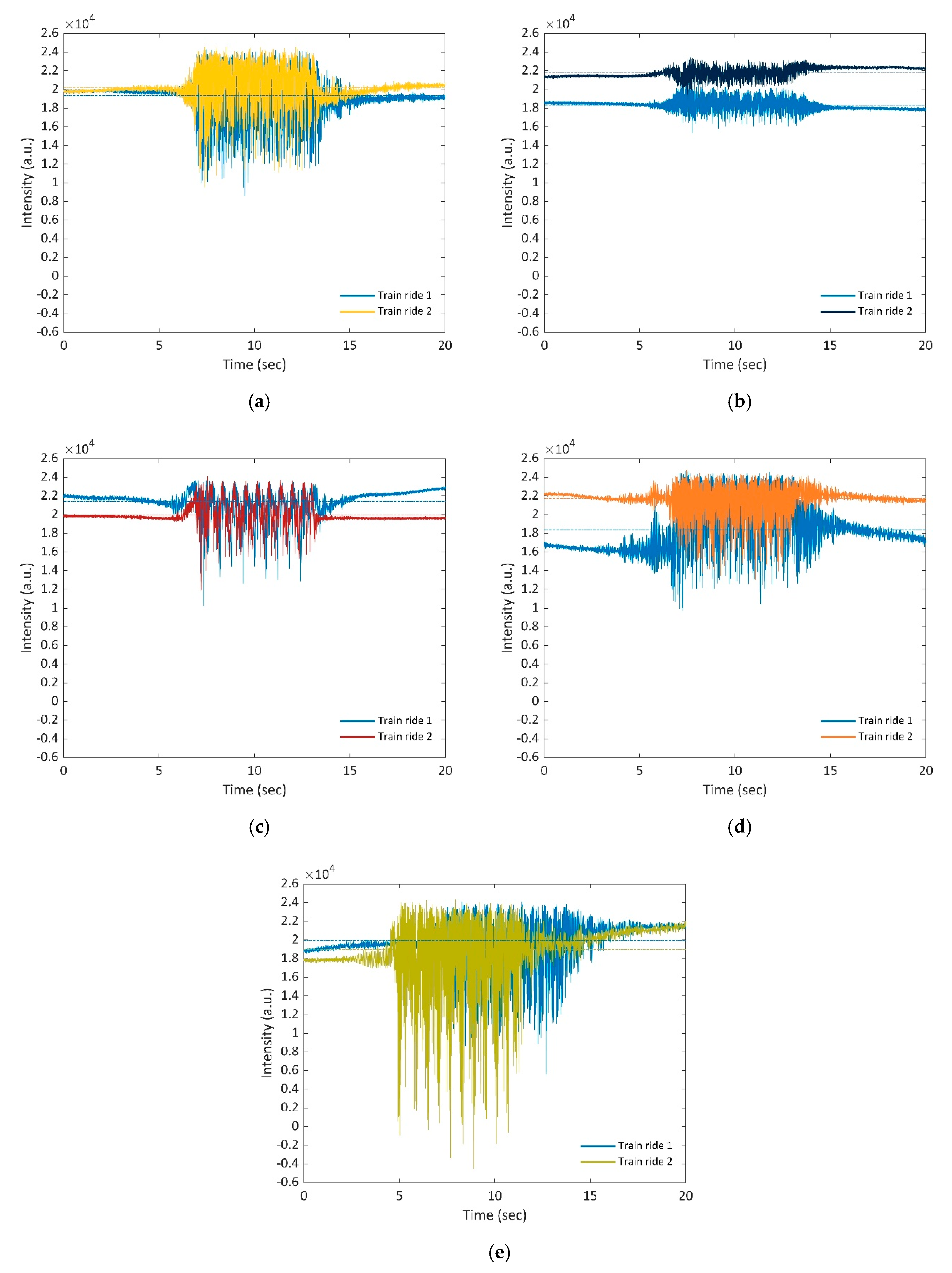
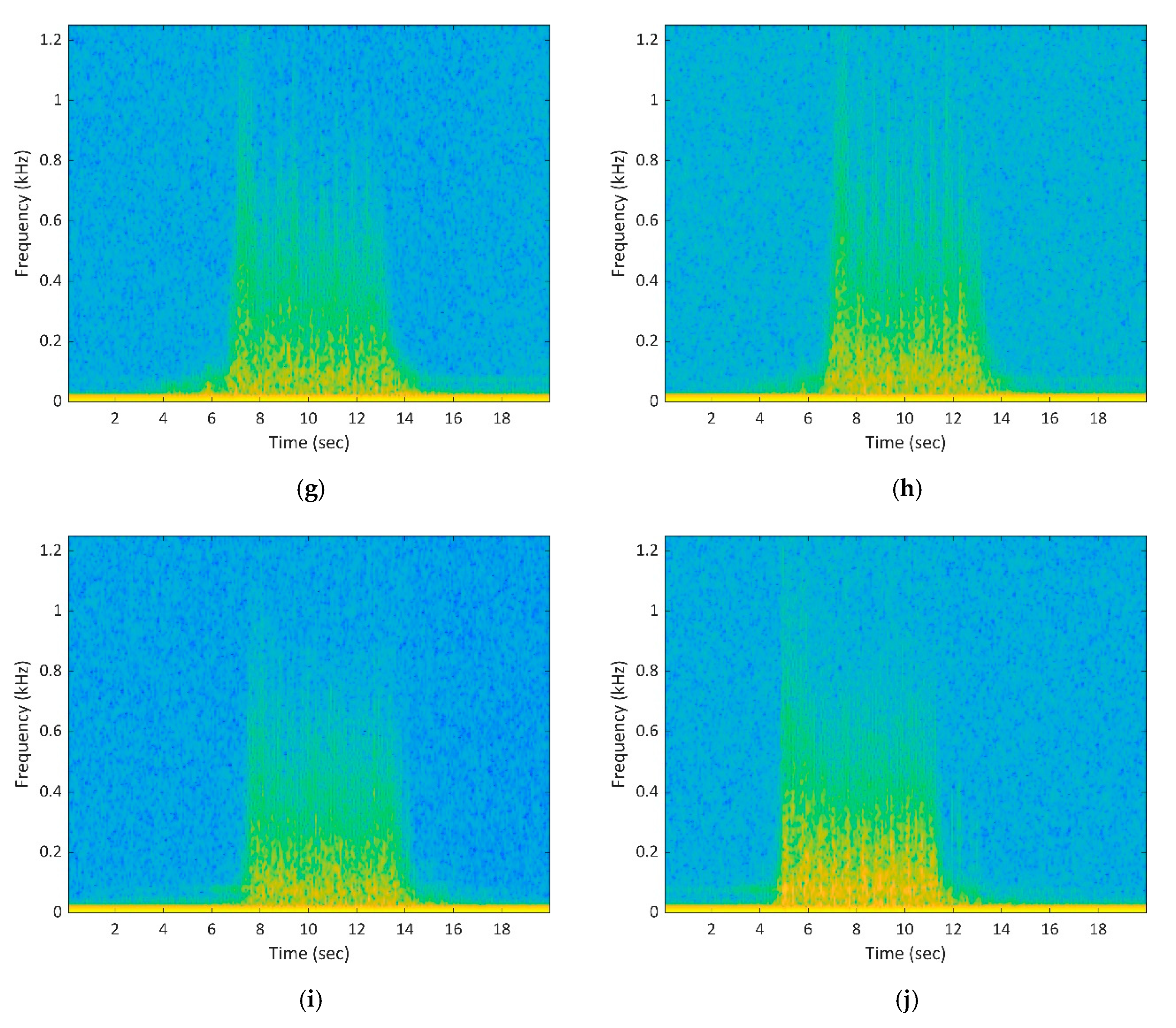
4.2. Signal Pattern and Properties of Two Trains in the Same Composition at the Same Channels (Location)

While the signal pattern differs for the same train journey among the channels, a question arises on whether the scattering process is similar for the same train composition at the same channel where the time difference between the two train rides is approximately one hour.

The comparative analysis reveals a completely different scattering process taking place in all the channels displayed in Figure 5a–e. While the pattern seems to correlate for at least both the train journeys in the same train composition in the respective channel, it differed among the channels significantly even though the travelling speeds did not vary much. The scatterings shown in Figure 5a,c are almost congruent for both trains, showing that they had a similar impact on the signal. The same also applies, in a diluted form, to the train journeys in Figure 5b,d,e, regardless of the contrasting signal pattern between the channels.

On analysis, the signal two circumstances are striking: (1) Channel 325 showed the least distinct scattering and, (2) while the values for the first four channels do not fall below zero, this was not true for Channel 399, where the smallest value was far below zero (−4552). The statistical values of both train rides are listed in

Table 3. Statistical values of the measurement as two trains in the same composition pass through channels 300, 325, 350, 375 and 399 on the same day.

	Raw Signal
	Train Ride 1					Train Ride 2
	300	325	350	375	399	300	325	350	375	399
Min (a.u.)	8546	15,346	10,245	9708	5593	9521	18,949	11,869	13,022	−4552
Max (a.u.)	24,299	20,910	23,683	24,638	24,140	24,578	23,491	24,093	24,809	24,369
Mean (a.u.)	19,355	18,316	21,407	18,383	19,948	20,206	21,845	19,930	21,720	18,949
SD (a.u.)	1496	509	1392	2380	1898	1344	525	1128	1042	2835

.

The results show that approaching trains, regardless of type, composition, speed and condition, have an immediate impact on the scattering process taking place in the fibre, resulting in a changed signal pattern in the time-domain. To determine whether the frequency response of the signal also changes due to the impact of a train, spectrograms were generated for a result visualisation using Matlab. In the first step, the signal was divided into overlapping segments and afterwards each segment was windowed with a Kaiser window (we used the default settings from Matlab). Subsequently, a short-time Fourier transform was computed, and the results were concatenated. The length of the segments (time resolution) and the amount of overlap between adjoining segments can be varied. In this case, we have chosen an overlap (specified as a percentage of the segment length) of 50%, with a time resolution of 78.4 ms. The frequency resolution was 32.7391 Hz. In basic terms, this is a histogram in a power-frequency space where a specific frequency appears brighter and “hotter” for as long as it persists in the signal while the signal is evolving. Based on the Nyquist theorem, the sampling rate of a signal must be at least twice the highest analogue frequency component. The utilised system had a sampling rate of 2500 samples per second, which meant that the highest detectable frequency was 1.25 kHz.

Spectrograms were calculated for the same channels as in the figures below. On the left, the spectrogram of Train Journey 1 is depicted and on the right Train Journey 2 can be seen. The y-axis represents the frequency of the signal and the x-axis represents the time. Firstly, frequencies up to approximately 40 Hz are steadily present even without a train movement as is clearly visible and thus frequencies up to 0.04 kHz can be classified as noisy (continuously present over the entire time). When a train approaches and passes the specific channel between second seven and 14, as displayed in Figure 6a, higher frequencies were also present and emerged due to the train’s sound and vibrations. A closer look at the frequency spectrum reveals the impact of at least each bogie emphasised by the “yellowish” peaks. The frequency spectrum of channel 300 for Train Journeys 1 and 2 is almost the same, meaning that the system measures the same regardless of the Train Journey. This is confirmed by the results of the other channels as a similar effect can be observed for the other channels too. Another very interesting result relates to the time-domain analyses of the backscattered intensity (see figures before) and the frequency content of the respective channels (see figures below). The signal would appear to be relatively more stable in the frequency domain than in the time domain, which is underpinned by the results illustrated in Figure 6. These only minor changes in the frequency properties, of course, can occur due to various reasons but, the signal seems to be more reliable in the frequency domain.

The train type, condition and speed undoubtedly affect the signal pattern, scattering behaviour and, consequently, the frequency content. Equally important, however, is the influence of the infrastructure and its condition. External perturbations and local conditions change the signal properties providing the user with essential information on boundary conditions. Otherwise, the sensing system could not be used for condition monitoring, intrusion monitoring and many other applications. Ensuring the pipeline integrity, the detection of immediate leakages and risk mitigation, for example, are very common applications for DAS, because pipelines are linear assets. The influence of the infrastructure on the signal properties can best be demonstrated by simply comparing the results depicted in the figures above (Figure 5 and Figure 6). Each channel corresponds to a certain position of the monitored track. Channel 300, depicted in Figure 5a and Figure 6a,b, are linked to a straight section with concrete sleepers. The scattering is quite characteristic and shows a distinctive pattern. As mentioned previously, the train-related signal content and noise were visible up to frequencies of 300–400 Hz, but the impact of the vehicle and the response of the infrastructure are very clear. The locomotive is the heaviest vehicle in the train composition, but shorter bogie distances made it difficult to identify the impact of each axle. Nevertheless, at least two high values were visible. The bogie distance was greater for the coaches, and they are thus more easily recognized. When compared to the results above, the scattering in Channel 325 and 350 (Figure 6c–f) changes significantly. However, when only 250 and 500 m away from Channel 300, the two measurements show no correlation. A question then arises regarding the reasons for the drastically changed measurement results. This issue can be resolved by linking the asset data, both the fibre and track layout and channel position. Channel 325 lies within a station and Channel 350 is in the middle of a coil where both seem to have no sensing capabilities at all. The scattering occurring at a position only 250 m further away (again straight section and concrete sleepers) once more delivers a completely different signal pattern (Figure 6g,h). This channel showed not only a very prominent peak dispersion, but also seemed to be very noisy. The same applies for the scattering observed in Channel 399. In contrast to Channel 300, neither the number of vehicles nor the impact of single bogies or axles could be identified. In this case, the train ride is visible, and the signal was constantly present up to a frequency of ~0.4 kHz. Higher frequencies were hardly present though.

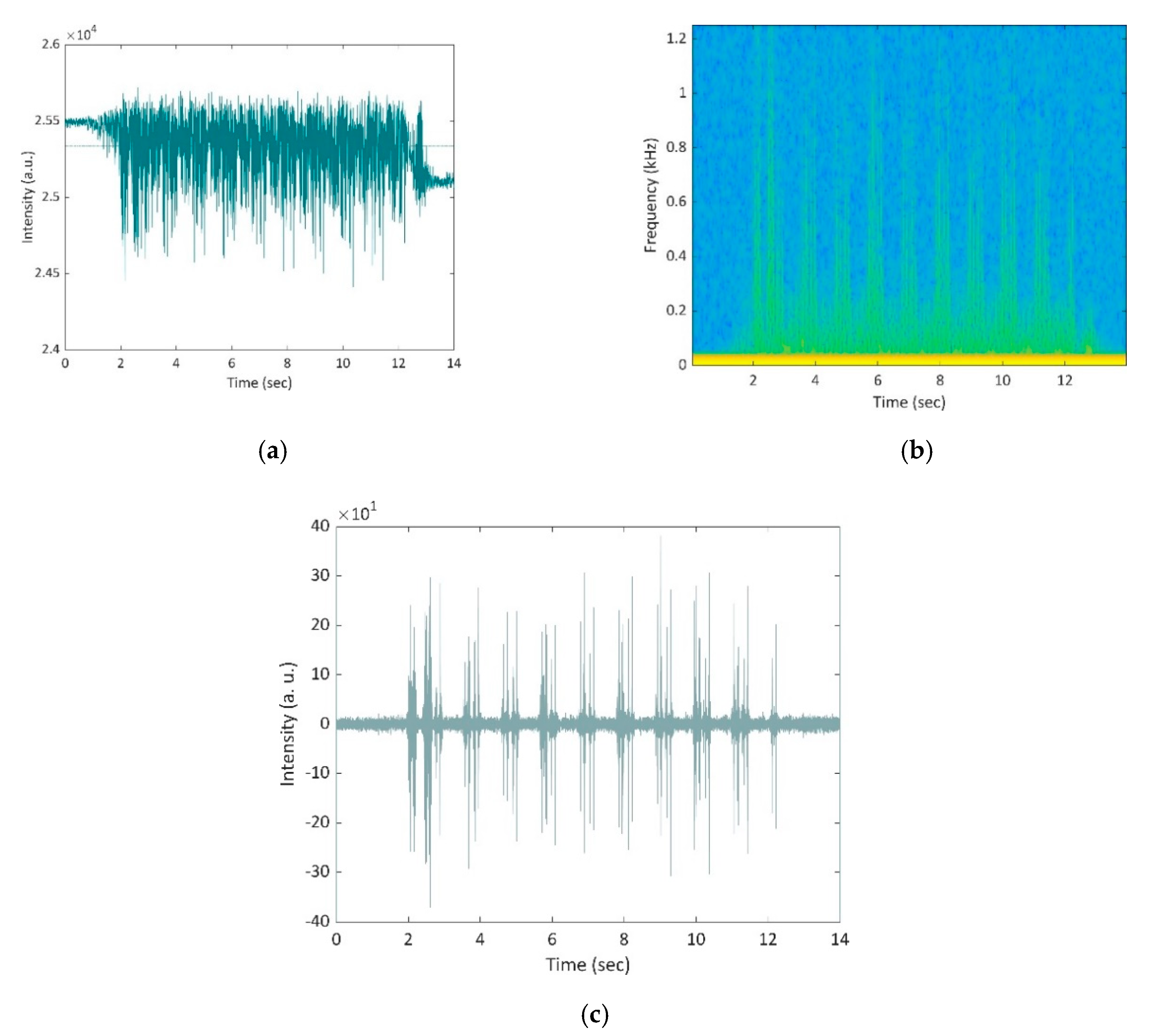
4.3. Signal Pattern and Properties When a Train Passes an Insulated Rail Joint in an Advanced State of Wear

The last position analysed was linked to an insulated rail joint (IRS) showing an advanced state of wear. The measurements revealed a scattering completely in contrast (Figure 7) to those analysed previously. Firstly, no extensive peaks could be observed when analysing the backscattered signal. In fact, the scattering showed no characteristic properties and the signal seems to be weak. While high peak values could previously be identified, this was no longer the case at this position. A reason for this could be that it is almost the 20th km of IU2. However, an already weakened signal after only 20 km does not appear to be a very reasonable assumption. On analysing the spectrogram of the channel, the picture completely changes. Before the train approached and passed the channel, frequencies up to approximately 0.04 kHz were steadily present containing no valuable information. This corresponds very well to the results obtained previously. At the moment the train entered the channel, the backscattered signal was altered, and the frequency content changed (Figure 7b). In this specific case, higher frequencies were observed as a result of the infrastructure response to the train passing the worn-out rail joint. The first yellowish peaks arose due to the impact of the locomotive’s bogies and axles followed by the coaches it was pulling. Higher frequencies were no longer present as the train travelled further and no axle passes the specific point. Consequently, frequencies up to ~0.3 kHz only were visible and can be considered as the train specific signature. As the next axle and bogie passed the rail joint, immediate responses to the impact and higher frequencies were present again. While the raw backscattered intensity has a remarkable behaviour, the filtered signal exposes a different picture. The use of a Butterworth high-pass filter (HPF) third order with a 400 Hz cut-off frequency removed all lower frequencies, allowing only frequencies higher than 400 Hz to pass. The impact of not only each bogie but rather of every single axle was unambiguously identifiable and the vehicles forming this train were countable, while it was also evident that all noise has been removed by applying an HPF (Figure 7c). Each time an axle or at least a bogie passed the rail joint, the infrastructure reacted to the impact of the load. The depicted train formation consisted of a locomotive and nine coaches and is, in fact, the reference train. The first four peaks arose due to the load of the locomotive, which also had shorter bogie distances compared to that of the following coaches. Additionally, knowing that the total length of the passing train that was 259.7 m (9 coaches each 26.8 m long and a locomotive with a length of 18.5 m) and the passage took slightly more than ten seconds, the travelling speed at this point could be calculated (~94 km/h).

5. Conclusions and Discussion

Utilising and adapting existing infrastructure—in this specific case, the infrastructure of deployed optical fibres alongside railway tracks—for sensing and consequently monitoring the condition of railway infrastructure represents a promising data source, for infrastructure managers to increase the information volume and gain knowledge about their asset condition. The network of installed optical fibres covers wide parts of the infrastructure primarily used for telecommunication and signalling to date. Hence, connecting one dark fibre to an interrogator unit discloses all relevant events taking place on or in the proximity of linear infrastructures. This already constitutes a valuable information source for infrastructure managers since it enables them to monitor the infrastructure in question in real-time and can react immediately in case of disruptions. The sensing principle is a reaction to external perturbations resulting in an altered backscatter which makes it possible to conclude whether an unusual event has occurred at a specific position. The results outline the enormous potential of the sensing system but continued serious efforts must made in order to derive valid results. In general, the results presented confirm the system’s capability to track the condition monitoring and identification of isolated track defects. The fibre is highly sensitive to external perturbations leading to significantly different scatterings taking place within the cable. This shows that it is of crucial importance to know the root cause of the changed scattering processes and where they occurred along the track. Therefore, the identification of the optical fibre cable layout and its link to the track is mandatory in any case regardless whether using already installed fibres or solely for railway infrastructure condition monitoring deployed ones. Nevertheless, optical fibres alongside railway tracks do not always run parallel to the track because the distance between the cable guiding duct and the track varies. In addition, the fibre layout changes in complex areas such as stations or multitracked sections.

The FOS signal is affected by several circumstances changing both the sensing properties of the system and the scattering. One reason can be found in the sensing set up, because a dark fibre of already installed optical cables is utilised. A modified and customised experimental arrangement may lead to less random signal patterns and thus to more precise measurements. Nevertheless, some hurdles can be overcome by developing a methodology which allows a like-with-like comparison of and finally drawing consistent conclusions on the system’s capability for infrastructure condition monitoring. An example of a feasible approach to tackle this issue is presented here where the results presented so far proved that the measurement method can derive valuable information on areas of interest.

As shown, each train type produces a different signal pattern leading to a specific signal characteristic. The FOS signal changes in a remarkable manner over a given time as well as within a day of two train journeys in the same train composition. This may happen due to several reasons/conditions and some of these can be overcome with a methodology that always enables a like-with-like comparison. An effort to classify these influences is made as follows:

• Infrastructure condition.
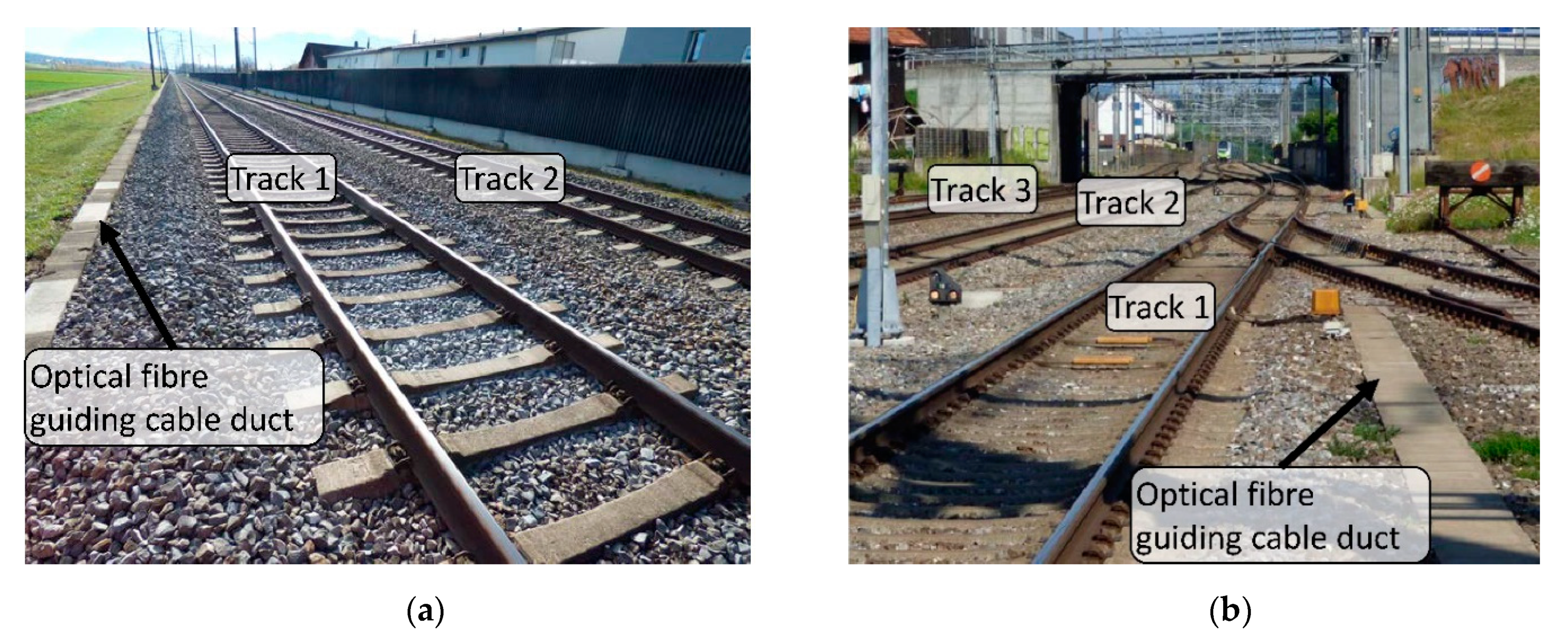
• Location, position and fixation of optical fibre cable.
• Properties of optical fibre cable.
• Train condition/properties.
• Random effects.
• Sensing properties.

The location, position and the type of fixation of the optical fibre certainly influence the sensing properties as well as the properties of the fibre. While these parameters are closely linked to the fibre itself, further parameters are assigned to both infrastructure and trains. To be more specific in the case of the latter, the wheel condition of a train, the train composition, loading status and speed certainly influence the backscattered intensity and therefore also affect the signal pattern. In the case of the infrastructure, its condition, superstructure and substructure will certainly have an impact on the signal. Further factors regarding the signal characteristics emerge due to random effects (phase in the sinus wave) and sensor effects (especially sensor noise). The data volume is always critical as further aspects need to be covered when using DAS in operation. These include considerations in the contexts of data mining, data processing and finally data storage. The question to be answered here is which values should be stored. The sensing principle shows the response of the infrastructure to the load induced by train movements, all of which vary among the different train types and compositions. Linked to this issue is also the integration of DAS data into existing system architectures and, probably the more important aspect—what data needs to be stored. Considering the huge data quantity that must be dealt with (a terabyte of raw data for just one day), it may be expedient to delete all processed/raw data and to retain only some statistical values. Additionally, also connected to this issue is the automated starting procedure for the measurements. If DAS is used for condition monitoring, it is feasible to record only those train movements that are of interest and, consequently, to reduce the data volumes on a precisely selected basis.

In general, examinations focusing on the frequency content of a signal and applying several digital filters make it possible to distinguish between the condition of different assets and sections. The results presented in this work point out that the system can distinguish between different asset conditions and detect track defects. The shortcomings of the applied technology are the inability of assigning a signal pattern explicitly to a specific failure/defect and to make a conclusion about the actual track geometry. Nevertheless, the latter is not necessarily mandatory, since track recording vehicles are designed to fulfil this task. In order to identify a specific failure, more defects of the same type are necessary and allow for an unequivocal identification. In combination with asset data, this permits one to draw conclusions regarding the reason for signal anomalies and to respond by carrying out the maintenance tasks required. The more sophisticated approach poses phase-sensitive systems, as they show promising results in fault detection and the identification of such. Furthermore, as phase-sensitive systems (quantitative measurements) are considered state-of-the art systems, most of the research and development focusses on these systems. However, quantitative systems have also some disadvantages, namely a shorter sensing length (compared to qualitative systems) and increased data amount, but suppliers and researching institutes are focusing on solving these issues at the moment. However, it does not matter whether a qualitative or a quantitative system is used and applied, the results prove the ability of distributed acoustic sensing for the monitoring of infrastructure conditions.

References

1. Marschnig, S.; Veit, P.; Girsch, G.; Eichberger, P. LCC-optimised permanent way strategies for track and turnout components. ZEVrail 2006, 130, 500–508. [Google Scholar]
2. Auer, F. Multi-function Track Recording Cars. Available online: https://www.plasser.com.br/fileadmin/user_upload/Mediathek/Publikationen/32_36_Auer.pdf (accessed on 10 June 2020).
3. Yazawa, E.; Takeshita, K. Development of Measurement Device of Track Irregularity using Inertial Mid-chord Offset Method. Q. Rep. RTRI 2002, 43, 125–130. [Google Scholar] [CrossRef] [Green Version]
4. Erhard, F.; Wolter, K.U.; Zacher, M. Improvement of track maintenance by continuous monitoring with regularly scheduled high speed trains. In Proceedings of the Railway Engineering–10th International Conference & Exhibition 2009, London, UK, 24–25 June 2009. [Google Scholar]
5. McAnaw, H.E. The system that measures the system. NDT E Int. 2003, 36, 169–179. [Google Scholar] [CrossRef]
6. Weston, P.F.; Ling, C.S.; Goodman, C.J.; Roberts, C.; Li, P.; Goodall, R.M. Monitoring lateral track irregularity from in-service railway vehicles. Proc. Inst. Mech. Eng. Part F J. Rail Rapid Transit 2007, 221, 89–100. [Google Scholar] [CrossRef]
7. Westeon, P.F.; Ling, C.S.; Roberts, C.; Goodman, C.J.; Li, P.; Goodall, R.M. Monitoring vertical track irregularity from in-service railway vehicles. Proc. Inst. Mech. Eng. Part F J. Rail Rapid Transit 2007, 221, 75–88. [Google Scholar] [CrossRef]
8. Kassa, E.; Sramota, J.; Kaynia, A. DESTination RAIL—Decision Support Tool for Rail Infrastructure Managers: D1.3 Report on Monitoring Switches and Crossings. 2017. Available online: https://cordis.europa.eu/project/id/284995 (accessed on 10 June 2020).
9. Loendersloot, R.; Mostafa, N. DESTination RAIL—Decision Support Tool for Rail Infrastructure Managers: D1.5 Implementation of a Complete Vibration Monitoring System on Irish Rail Bridge. 2018. Available online: https://cordis.europa.eu/project/id/284995 (accessed on 10 June 2020).
10. Barke, D.; Chiu, K.W. Structural health monitoring in the railway industry: A review. Struct. Heal. Monit. 2005, 4, 81–94. [Google Scholar] [CrossRef]
11. Kantamaa, S.M.V. Wayside train monitoring system—A multitask database for asset owners. Signal Draht 2015, 11, 31–35. [Google Scholar]
12. Maiman, T.H. Stimulated optical radiation in Ruby. Nature 1960. [Google Scholar] [CrossRef]
13. Kao, K.C.; Hockham, G.A. Dielectric-fibre surface waveguides for optical frequencies. Proc. Inst. Electr. Eng. 1966, 113, 1151–1158. [Google Scholar] [CrossRef] [Green Version]
14. Kapron, F.P.; Keck, D.B.; Maurer, R.D. Radiation losses in glass optical waveguides. Appl. Phys. Lett. 1970, 17, 423. [Google Scholar] [CrossRef]
15. Udd, E.; Spillman, B., Jr. Fiber Optic Sensors: An Introduction for Engineers and Scientists, 2nd ed.; John Wiley & Sons: Hoboken, NJ, USA, 2011; ISBN 978-0-470-12684-4. [Google Scholar]
16. Lee, K.Y.; Lee, K.K.; Ho, S.L. Exploration of using FBG sensor for derailment detector. WSEAS Trans. Top. Syst. 2004, 3, 2433–2439. [Google Scholar]
17. Lee, K.Y.; Lee, K.K.; Ho, S.L. Exploration of Using FBG Sensor for Axle Counter in Railway Engineering. WSEAS Trans. Top. Syst. 2004, 6, 2440–2447. [Google Scholar]
18. Filograno, M.L.; Corredera, P.; Rodriguez-Plaza, M.; Andres-Alguacil, A.; González-Herráez, M. Wheel Flat Detection in High-Speed Railway Systems Using Fiber Bragg Gratings. IEEE Sens. J. 2013, 13, 4808–4816. [Google Scholar] [CrossRef]
19. Roveri, N.; Carcaterra, A.; Sestieri, A. Real-time monitoring of railway infrastructures using fibre Bragg grating sensors. Mech. Syst. Signal Process. 2015, 60–61, 14–28. [Google Scholar] [CrossRef]
20. Mennella, F.; Laudati, A.; Esposito, M.; Cusano, A.; Cutolo, A.; Giordano, M.; Campopiano, S.; Breglio, G. Railway monitoring and train tracking by fiber Bragg grating sensors. In Proceedings of the Third European Workshop on Optical Fibre Sensors, Napoli, Italy, 4–6 July 2007; SPIE: Bellingham, WA, USA, 2007; Volume 6619, p. 66193H. [Google Scholar] [CrossRef]
21. Mi, Q.; Gao, X.; Zhu, H.; Wang, Z.; Zhao, Q. Composite railway health monitoring system based on fiber optic bragg grating sensing array. In Proceedings of the 2014 IEEE Far East Forum on Nondestructive Evaluation/Testing, Chengdu, China, 20–23 June 2014; pp. 259–264. [Google Scholar] [CrossRef]
22. Kinet, D.; Kouroussis, G.; Dupuy, J.; Moeyaert, V.; Verlinden, O.; Caucheteur, C. Cost-effective FBG interrogation combined with cepstral-based signal processing for railway traffic monitoring. In Proceedings of the Optical Sensing and Detection IV, Brussels, Belgium, 3–7 April 2016. [Google Scholar] [CrossRef]
23. Kouroussis, G.; Kinet, D.; Moeyaert, V.; Dupuy, J.; Caucheteur, C. Railway structure monitoring solutions using fibre Bragg grating sensors. Int. J. Rail Transp. 2016, 4, 135–150. [Google Scholar] [CrossRef]
24. Wang, P.; Xie, K.; Shao, L.; Yan, L.; Xu, J.; Chen, R. Longitudinal force measurement in continuous welded rail with bi-directional FBG strain sensors. Smart Mater. Struct. 2016, 25, 015019. [Google Scholar] [CrossRef]
25. Kang, D.; Kim, D.-H.; Jang, S. Design and Development of Structural Health Monitoring System for Smart Railroad-Gauge-Facility Using FBG Sensors. Exp. Tech. 2012, 38, 39–47. [Google Scholar] [CrossRef]
26. Zhang, Y.; Liu, F.; Jing, Y.; Li, W. Application of FBG sensing technique for monitoring and early warning system of high-speed railway track conditions. In Proceedings of the 25th International Conference on Optical Fiber Sensors, Jeju, Korea, 24–28 April 2017. [Google Scholar] [CrossRef]
27. Hussaini, S.K.K.; Indraratna, B.; Vinod, J.S. Application of optical-fiber bragg grating sensors in monitoring the rail track Deformations. Geotech. Test. J. 2015, 38, 387–396. [Google Scholar] [CrossRef] [Green Version]
28. Lai, C.C.; Au, H.Y.; Liu, M.S.Y.; Ho, S.L.; Tam, H.Y. Development of Level Sensors Based on Fiber Bragg Grating for Railway Track Differential Settlement Measurement. IEEE Sens. J. 2016, 16, 6346–6350. [Google Scholar] [CrossRef]
29. Buggy, S.J.; James, S.W.; Staines, S.; Carroll, R.; Kitson, P.V.; Farrington, D.; Drewett, L.; Jaiswal, J.; Tatam, R.P. Railway track component condition monitoring using optical fibre Bragg grating sensors. Meas. Sci. Technol. 2016, 27, 055201. [Google Scholar] [CrossRef] [Green Version]
30. Scott, R.H.; Banerji, P.; Chikermane, S.; Srinivasan, S.; Basheer, P.A.M.; Surre, F.; Sun, T.; Grattan, K.T.V. Commissioning and evaluation of a fiber-optic sensor system for bridge monitoring. IEEE Sens. J. 2013, 13, 2555–2562. [Google Scholar] [CrossRef] [Green Version]
31. Wei, Y.J.; Zhang, J.T.; Zhang, Y.L.; Xi, X.C.; Li, K.; Liu, S.C. Research on evaluation method of the bridge strengthening effect based on fiber optic sensor. Adv. Mater. Res. 2013, 791–793, 1901–1904. [Google Scholar] [CrossRef]
32. Bocciolone, M.; Bucca, G.; Collina, A.; Comolli, L. Pantograph–catenary monitoring by means of fibre Bragg grating sensors: Results from tests in an underground line. Mech. Syst. Signal Process. 2013, 41, 226–238. [Google Scholar] [CrossRef]
33. Wagner, R.; Maicz, D.; Viel, W.; Saliger, F.; Saliger, C.; Horak, R.; Noack, T. A fibre optic sensor instrumented pantograph as part of a continuous structural health monitoring system for railway overhead lines. In Proceedings of the 7th European Workshop on Structural Health Monitoring, EWSHM 2014-2nd European Conference of the Prognostics and Health Management (PHM) Society, Nantes, France, 8–11 July 2014. [Google Scholar]
34. Catalano, A.; Bruno, F.A.; Galliano, C.; Pisco, M.; Persiano, G.V.; Cutolo, A.; Cusano, A. An optical fiber intrusion detection system for railway security. Sens. Actuators A Phys. 2017, 253, 91–100. [Google Scholar] [CrossRef]
35. Esposito, F.; Zotti, A.; Palumbo, G.; Zuppolini, S.; Consales, M.; Cutolo, A.; Borriello, A.; Campopiano, S.; Zarrelli, M.; Iadicicco, A. Liquefied petroleum gas monitoring system based on polystyrene coated long period grating. Sensors 2018, 18, 1435. [Google Scholar] [CrossRef] [PubMed] [Green Version]
36. Rogers, A. Distributed optical-fibre sensing. Meas. Sci. Technol. 1999, 10, R75–R99. [Google Scholar] [CrossRef]
37. Boyd, R.W. Nonlinear Optics; Academic Press: Cambridge, MA, USA, 2008; ISBN 9780123694706. [Google Scholar]
38. Santos, J.L.; Farahi, F. Handbook of Optical Sensors; CRC Press: Boca Raton, FL, USA, 2014; ISBN 9780429193521. [Google Scholar]
39. Minardo, A.; Porcaro, G.; Giannetta, D.; Bernini, R.; Zeni, L. Real-time monitoring of railway traffic using slope-assisted Brillouin distributed sensors. Appl. Opt. 2013, 52, 3770–3776. [Google Scholar] [CrossRef] [PubMed]
40. Klug, F.; Lackner, S.; Lienhart, W. Monitoring of Railway Deformations Distributed Fiber Optic Sensors. In Proceedings of the 3rd Joint International Symposium on Deformation Monitoring (JISDM), Vienna, Austria, 30 March–1 April 2016; pp. 1–8. [Google Scholar]
41. Bao, Y.; Chen, G.; Meng, W.; Tang, F.; Chen, Y. Kilometer-Long Optical Fiber Sensor for Real-Time Railroad Infrastructure Monitoring to Ensure Safe Train Operation. In Proceedings of the 2015 Joint Rail Conference; American Society of Mechanical Engineers, San Jose, CA, USA, 23–26 March 2015. [Google Scholar] [CrossRef]
42. Wheeler, L.N.; Pannese, E.; Hoult, N.A.; Take, A.; Le, H. Measurement of distributed dynamic rail strains using a Rayleigh backscatter based fiber optic sensor: Lab and field evaluation. Transp. Geotech. 2018, 14, 70–80. [Google Scholar] [CrossRef]
43. Chapeleau, X.; Sedran, T.; Cottineau, L.-M.; Cailliau, J.; Taillade, F.; Gueguen, I.; Henault, J.-M. Study of ballastless track structure monitoring by distributed optical fiber sensors on a real-scale mockup in laboratory. Eng. Struct. 2013, 56, 1751–1757. [Google Scholar] [CrossRef]
44. Juarez, J.C.; Maier, E.W.; Choi, K.N.; Taylor, H.F. Distributed fiber optic intrusion sensor system. J. Light. Technol. 2005, 23, 2081–2087. [Google Scholar] [CrossRef]
45. Peng, F.; Duan, N.; Rao, Y.J.; Li, J. Real-time position and speed monitoring of trains using phase-sensitive OTDR. IEEE Photonics Technol. Lett. 2014, 26, 2055–2057. [Google Scholar] [CrossRef]
46. Lindsey, N.J.; Craig Dawe, T.; Ajo-Franklin, J.B. Illuminating seafloor faults and ocean dynamics with dark fiber distributed acoustic sensing. Science (80-) 2019, 366, 1103–1107. [Google Scholar] [CrossRef] [PubMed]
47. Mateeva, A.; Lopez, J.; Mestayer, J.; Wills, P.; Cox, B.; Kiyashchenko, D.; Yang, Z.; Berlang, W.; Detomo, R.; Grandi, S. Distributed acoustic sensing for reservoir monitoring with VSP. Lead. Edge 2013, 32, 1278–1283. [Google Scholar] [CrossRef]
48. Wang, Z.; Lu, B.; Zheng, H.; Ye, Q.; Pan, Z.; Cai, H.; Qu, R.; Fang, Z.; Zhao, H. Novel railway-subgrade vibration monitoring technology using phase-sensitive OTDR. In Proceedings of the 25th International Conference on Optical Fiber Sensors, Jeju, Korea, 24–28 April 2017. [Google Scholar] [CrossRef]
49. Barnoski, M.K.; Jensen, S.M. Fiber waveguides: A novel technique for investigating attenuation characteristics. Appl. Opt. 1976, 15, 2112–2115. [Google Scholar] [CrossRef] [PubMed]
50. Barnoski, M.K.; Rourke, M.D.; Jensen, S.M.; Melville, R.T. Optical time domain reflectometer. Appl. Opt. 1977, 16, 2375. [Google Scholar] [CrossRef] [PubMed]
51. Healey, P.; Booth, R.C.; Daymond-John, B.E.; Nayar, B.K. OTDR in single-mode fibre at 1.5 μm using homodyne detection. Electron. Lett. 1984, 20, 360. [Google Scholar] [CrossRef]
52. Healey, P.; Malyon, D.J. OTDR in single-mode fibre at 1.5 μm using heterodyne detection. Electron. Lett. 1982, 18, 862. [Google Scholar] [CrossRef]
53. Healey, P. Fading in heterodyne OTDR. Electron. Lett. 1984, 20, 30. [Google Scholar] [CrossRef]
54. Izumita, H.; Furukawa, S.i.; Koyamada, Y.; Sankawa, I. Fading Noise Reduction in Coherent OTDR. IEEE Photonics Technol. Lett. 1992, 4, 201–203. [Google Scholar] [CrossRef]
55. Izumita, H.; Koyamada, Y.; Furukawa, S.; Sankawa, I. Stochastic amplitude fluctuation in coherent OTDR and a new technique for its reduction by stimulating synchronous optical frequency hopping. J. Light. Technol. 1997, 15, 267–278. [Google Scholar] [CrossRef]
56. Shimizu, K.; Horiguchi, T.; Koyamada, Y. Characteristics and Reduction of Coherent Fading Noise in Rayleigh Backscattering Measurement for Optical Fibers and Components. J. Light. Technol. 1992, 10, 982–987. [Google Scholar] [CrossRef]
57. Lamb, C.; Dakin, J.P. Distributed Fibre Optic Sensor System. UK Patent GB2222247A, 28 February 1990. [Google Scholar]
58. Taylor, H.F.; Lee, C.E. Method For Fiber Optic Intrusion Sensing. U.S. Patent 5,194,847, 16 March 1993. [Google Scholar]
59. Juškaitis, R.; Mamedov, A.M.; Potapov, V.T.; Shatalin, S.V. Interferometry with Rayleigh backscattering in a single-mode optical fiber. Opt. Lett. 1994, 19, 225. [Google Scholar] [CrossRef] [PubMed]
60. Owen, A.; Duckworth, G.; Worsley, J. OptaSense: Fibre Optic Distributed Acoustic Sensing for Border Monitoring. In Proceedings of the 2012 European Intelligence and Security Informatics Conference, Odense, Denmark, 22–24 August 2012; pp. 362–364. [Google Scholar] [CrossRef]
61. Duckworth, G.; Owen, A.; Worsley, J.; Stephenson, H. Optasense® distributed acoustic and seismic sensing performance for multi-threat, multi-environment border monitoring. Proc. 2013 Eur. Intell. Secur. Inform. Conf. EISIC 2013, 2013, 273–276. [Google Scholar] [CrossRef]
62. Duckworth, G.L.; Ku, E.M. OptaSense distributed acoustic and seismic sensing using COTS fiber optic cables for infrastructure protection and counter terrorism. In Proceedings of the Sensors, and Command, Control, Communications, and Intelligence (C3I) Technologies for Homeland Security and Homeland Defense XII, Baltimore, MD, USA, 29 April–3 May 2013. [Google Scholar] [CrossRef]
63. Timofeev, A.V.; Egorov, D.V.; Denisov, V.M. The rail traffic management with usage of C-OTDR monitoring systems. Int. J. Comput. Electr. Autom. Control Inf. Eng. 2015, 9, 1492–1495. [Google Scholar] [CrossRef]
64. Timofeev, A. V Monitoring the Railways by Means of C-OTDR Technology. Int. J. Mech. Aerosp. Ind. Mechatron. Eng. 2015, 9, 586–589. [Google Scholar] [CrossRef]
65. Brauner, M.; Kogelnig, A.; Koenig, U.; Neunteufel, G.; Schilcher, H. Distributed acoustic monitoring to secure transport infrastructure against natural hazards—Requirements and new developments. In Proceedings of the Interpraevent 2016, Lucerne, Switzerland, 30 May–2 June 2016; pp. 231–238. [Google Scholar]
Figure 1. Typical spontaneous light scattering spectrum.
Applsci 10 06016 g001
Figure 2. (a) Schematic track and fibre layout of the monitored route between Bern Wankdorf and Spiez, located in Switzerland; (b) rack mounted interrogator units located in the telecommunications room in Muensingen side-by-side with the processing unit at the top.
Applsci 10 06016 g002
Figure 3. (a) Cable duct parallel to track 1 guiding and protecting the optical fibre. There is usually only one cable duct, located on the left-hand side of track 1, even though it is mostly a double-tracked line; (b) in the case of multitracked sections, one cable duct is provided whereby the fibre layout may change significantly, especially in the vicinity of bridges and turnouts, resulting in considerable fibre length excess.
Applsci 10 06016 g003
Figure 4. The backscattered intensity of the same train journey in 5 consecutive channels distributed equidistantly.
Applsci 10 06016 g004
Figure 5. Raw backscattered signal of two train rides in the same train composition on the same day in different channels (locations). (a) Channel 300; (b) Channel 325; (c) Channel 350; (d) Channel 375; (e) Channel 399.
Applsci 10 06016 g005
Figure 6. Spectrograms of two train journeys in the same composition in 5 consecutive channels distributed equidistantly. (a) Channel 300, Train journey 1; (b) Channel 300, Train journey 2; (c) Channel 325, Train journey 1; (d) Channel 325, Train journey 2; (e) Channel 350, Train journey 1; (f) Channel 350, Train journey 2; (g) Channel 375, Train journey 1; (h) Channel 375, Train journey 2; (i) Channel 399, Train journey 1; (j) Channel 399, Train journey 2.
Applsci 10 06016 g006aApplsci 10 06016 g006b
Figure 7. Raw backscattered signal (a), spectrogram (b) and filtered signal (c) of a train passing a rail joint in an advanced state of wear.
Applsci 10 06016 g007