Suitability of Active Noise Barriers for Construction Sites


Abstract
:1. Introduction
2. Theory
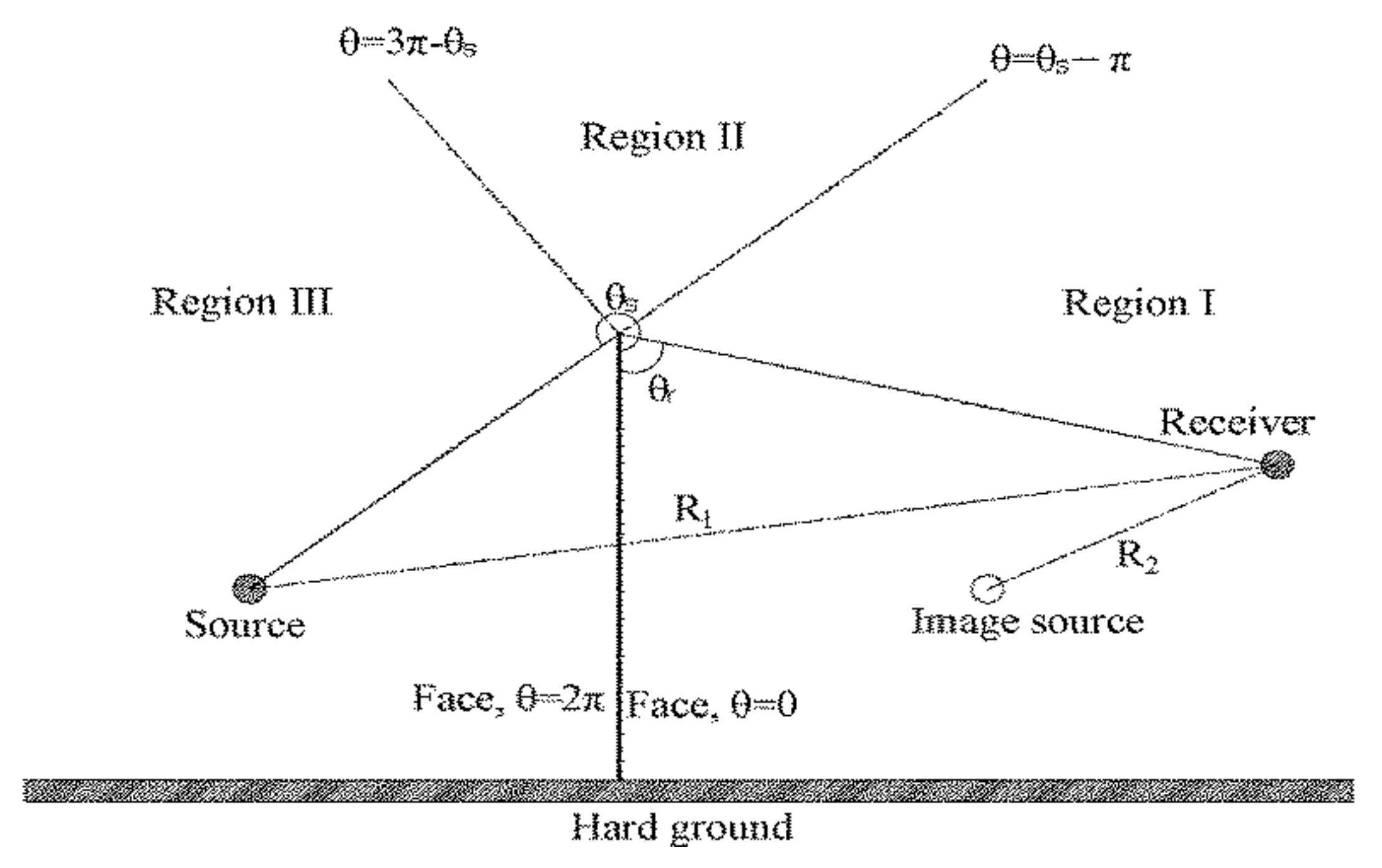
2.1. Diffraction Model
2.2. Active Noise Barriers
Minimization of Squared Pressure
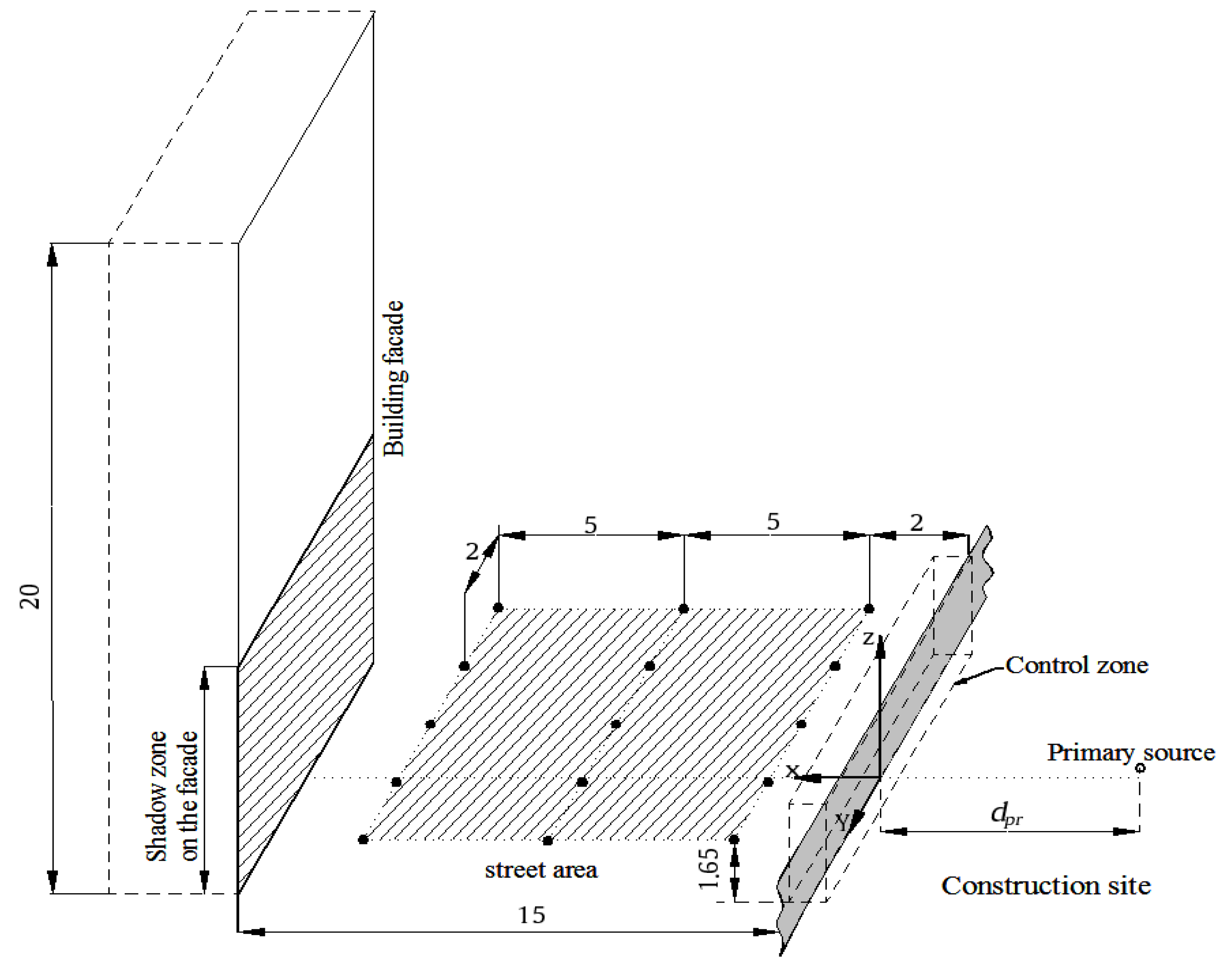
3. Method
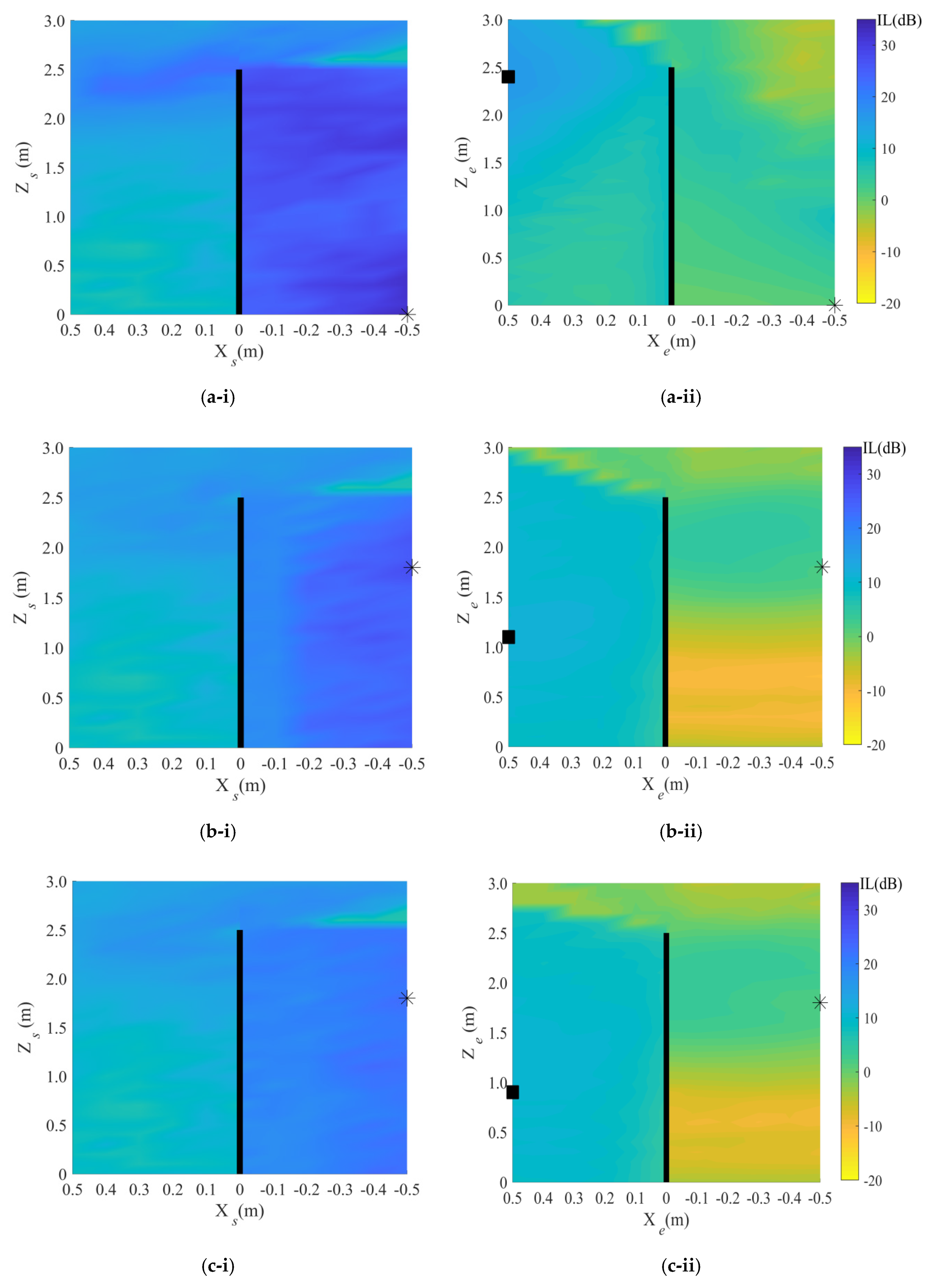
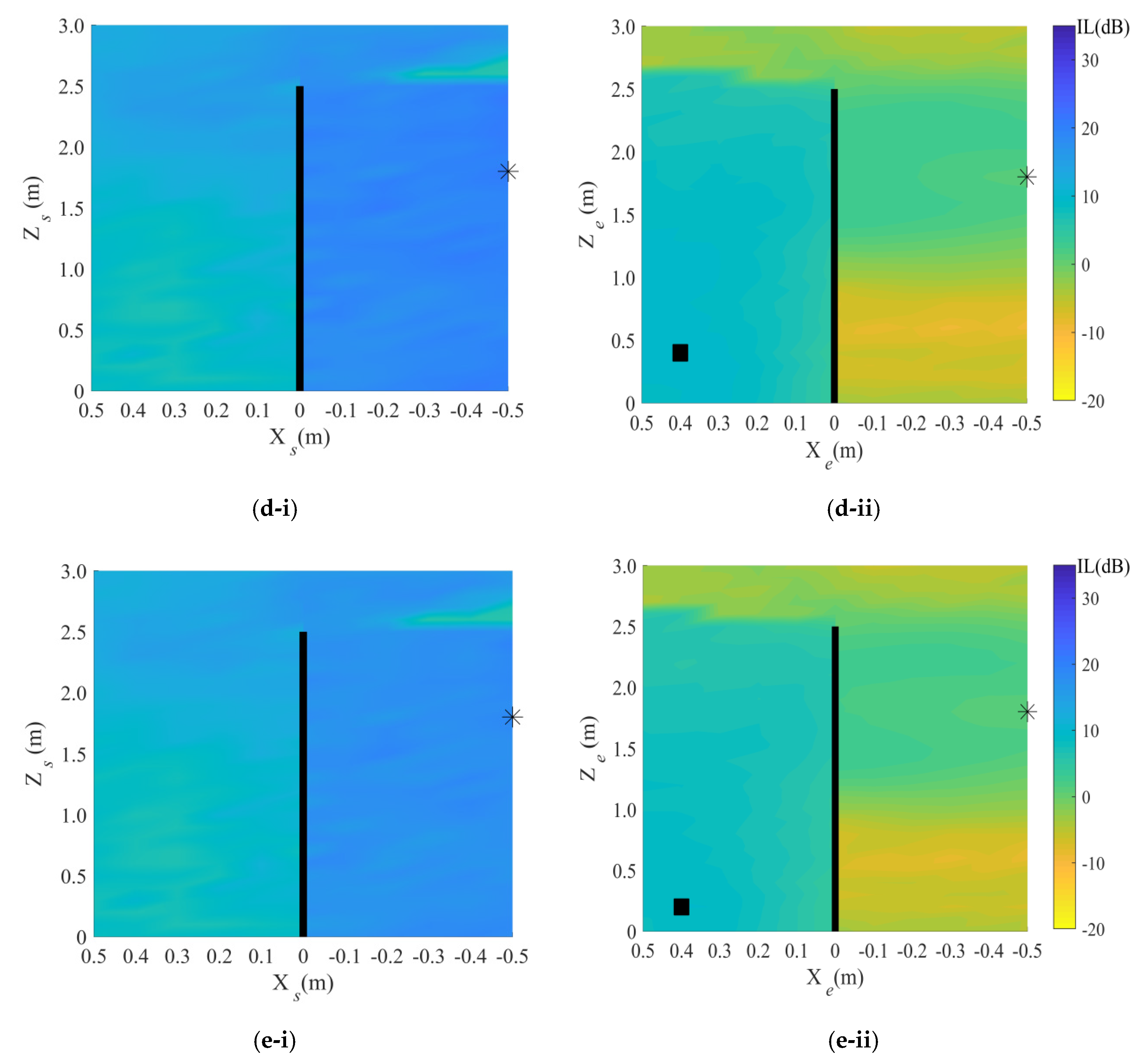
4. Results
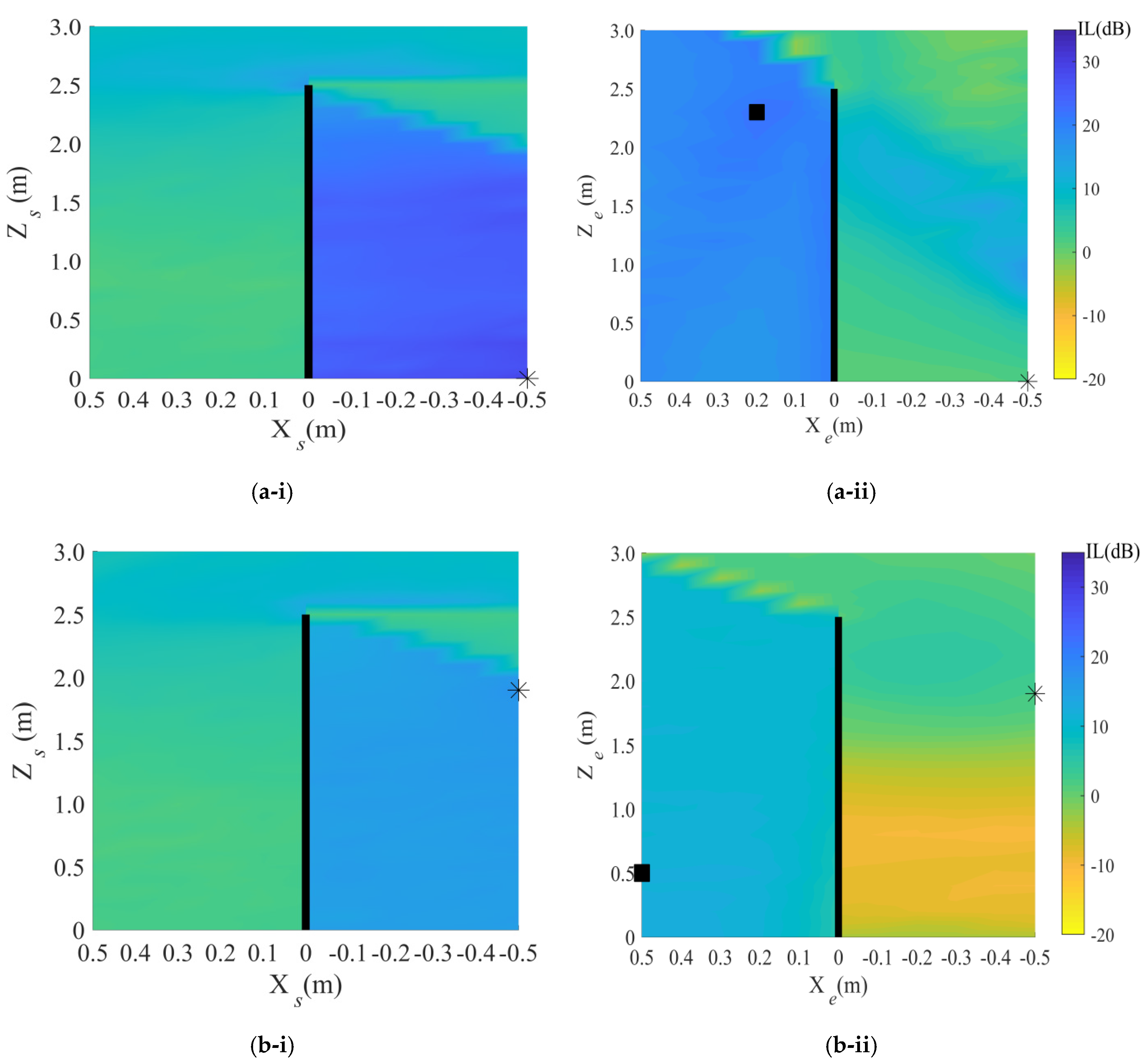
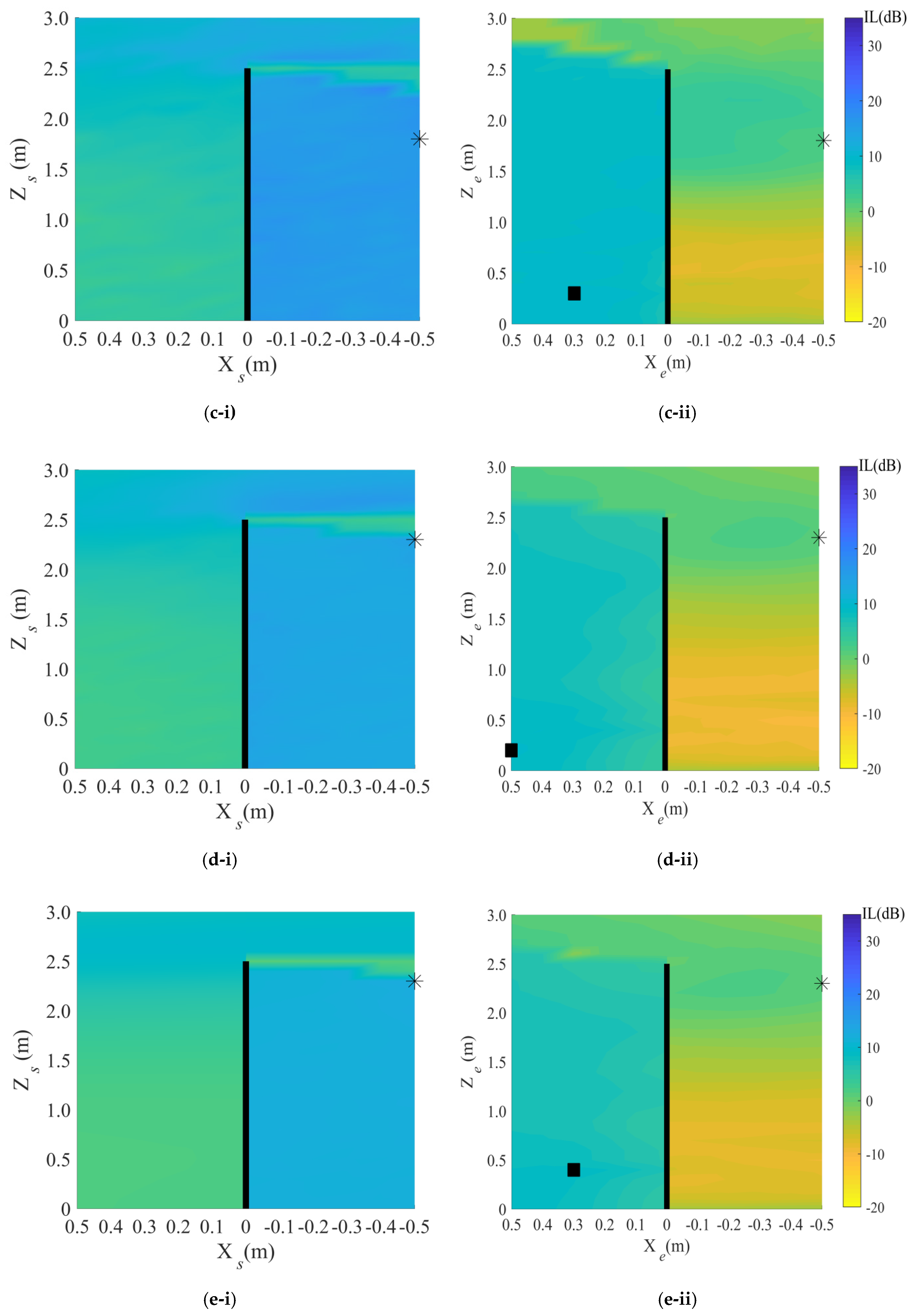
4.1. Target Area: Street Area
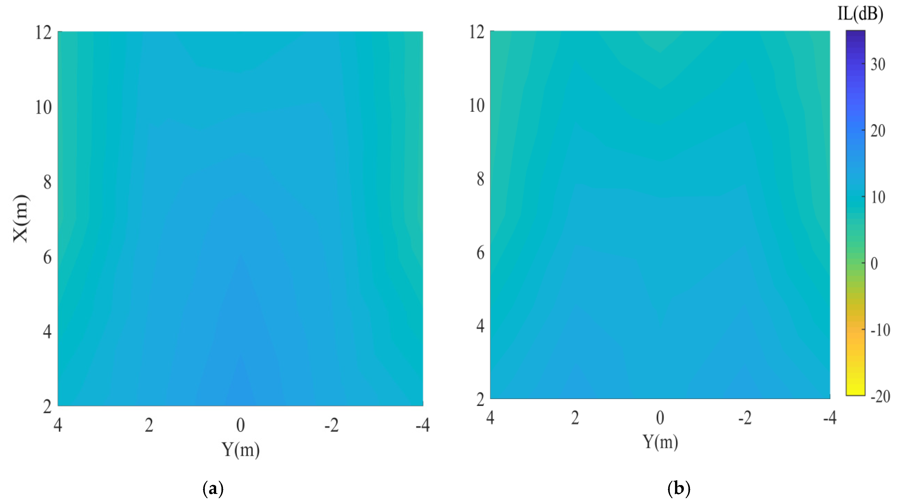
4.2. Target Area: Shadow Zone of the Façade
5. Discussion
5.1. Target Area: Street Area
5.2. Target Area: Shadow Zone of the Façade
6. Conclusions
Author Contributions
Funding
Acknowledgments
Conflicts of Interest
References
- Lee, S.C.; Kim, J.H.; Hong, J.Y. Characterizing perceived aspects of adverse impact of noise on construction managers on construction sites. Build. Environ. 2019, 152, 17–27. [Google Scholar] [CrossRef]
- Li, X.; Song, Z.; Wang, T.; Zheng, Y.; Ning, X. Health impacts of construction noise on workers: A quantitative assessment model based on exposure measurement. J. Clean. Prod. 2016, 135, 721–731. [Google Scholar] [CrossRef] [Green Version]
- Lee, S.C.; Hong, J.Y.; Jeon, J.Y. Effects of acoustic characteristics of combined construction noise on annoyance. Build. Environ. 2015, 92, 657–667. [Google Scholar] [CrossRef]
- Liu, Y.; Xia, B.; Cui, C.; Skitmore, M. Community response to construction noise in three central cities of Zhejiang province, China. Environ. Pollut. 2017, 230, 1009–1017. [Google Scholar] [CrossRef] [PubMed] [Green Version]
- Kwon, N.; Song, K.; Lee, H.-S.; Kim, J.; Park, M. Construction Noise Risk Assessment Model Focusing on Construction Equipment. J. Constr. Eng. Manag. 2018, 144, 1–12. [Google Scholar] [CrossRef]
- Ng, C.F. Effects of building construction noise on residents: A quasi-experiment. J. Environ. Psychol. 2000, 20, 375–385. [Google Scholar] [CrossRef] [Green Version]
- Ballesteros, M.J.; Fernandez, M.D.; Quintana, S.; Ballesteros, J.A.; González, I. Noise emission evolution on construction sites. Measurement for controlling and assessing its impact on the people and on the environment. Build. Environ. 2010, 45, 711–717. [Google Scholar] [CrossRef]
- Cheng, K.W.; Law, C.W.; Wong, C.L. Quiet construction: State-of-the-art methods and mitigation measures. In Proceedings of the Internoise 2014—43rd International Congress on Noise Control Engineering, Melbourne, Australian, 16–19 November 2014; pp. 1–10. [Google Scholar]
- Kwon, N.; Park, M.; Lee, H.-S.; Ahn, J.; Shin, M. Construction Noise Management Using Active Noise Control Techniques. J. Constr. Eng. Manag. 2016, 142. [Google Scholar] [CrossRef]
- Gilchrist, A.; Allouche, E.N.; Cowan, D. Prediction and mitigation of construction noise in an urban environment. Can. J. Civ. Eng. 2003, 30, 659–672. [Google Scholar] [CrossRef]
- Thalheimer, E. Construction noise control program and mitigation strategy at the Central Artery/Tunnel Project. Noise Control. Eng. J. 2000, 48, 157. [Google Scholar] [CrossRef] [Green Version]
- Zhaomeng, W.; Meng, L.K.; Priyadarshinee, P.; Pueh, L.H. Applications of noise barriers with a slanted flat-tip jagged cantilever for noise attenuation on a construction site. J. Vib. Control. 2017, 24, 5225–5232. [Google Scholar] [CrossRef]
- Ireland, T.I.; Centre, P.B.; Street, P. Noise management during the construction of a light rail scheme through Dublin city centre. In Proceedings of the INTER-NOISE 2019, Madrid, Spain, 16–19 June 2019. [Google Scholar]
- Wilson, P.M. Innovations that make infrastructure and construction noise control more effective. In Proceedings of the INTER-NOISE 2016—45th International Congress and Exposition on Noise Control Engineering, Hamburg, Germany, 21–24 August 2016. [Google Scholar]
- Lee, H.P.; Tan, L.B.; Lim, K.M. Assessment of the performance of sonic crystal noise barriers for the mitigation of construction noise. In Proceedings of the INTER-NOISE 2016—45th International Congress and Exposition on Noise Control Engineering, Hamburg, Germany, 21–24 August 2016; pp. 4220–4226. [Google Scholar]
- Lee, H.M.; Wang, Z.; Lim, K.M.; Lee, H.P. A Review of Active Noise Control Applications on Noise Barrier in Three-Dimensional/Open Space: Myths and Challenges. Fluct. Noise Lett. 2019, 18, 1–21. [Google Scholar] [CrossRef]
- Kanazawa, L.; Mizutani, K. Reduction of construction machinery noise in multiple dominant frequencies using feedforward type active control. In Proceedings of the INTER-NOISE 2018—47th International Congress and Exposition on Noise Control Engineering, Chicago, IL, USA, 26–29 August 2018. [Google Scholar]
- Chen, W.; Min, H.; Qiu, X. Noise reduction mechanisms of active noise barriers. Noise Control Eng. J. 2013, 61, 120–126. [Google Scholar]
- Han, N.; Qiu, X. A study of sound intensity control for active noise barriers. Phys. Appl. Acoust. 2007, 68, 1297–1306. [Google Scholar] [CrossRef]
- Guo, J.; Pan, J. Increasing the insertion loss of noise barriers using an active-control system. J. Acoust. Soc. Am. 1998, 104, 3408–3416. [Google Scholar] [CrossRef]
- Omoto, A. Active suppression of sound diffracted by a barrier: An outdoor experiment. J. Acoust. Soc. Am. 1997, 102, 1671–1679. [Google Scholar] [CrossRef]
- Rubio, C.; Castiñeira-Ibañez, S.; Uris, A.; Belmar, F.; Candelas, P. Numerical simulation and laboratory measurements on an open tunable acoustic barrier. Appl. Acoust. 2018, 141, 144–150. [Google Scholar] [CrossRef]
- Reiter, P.; Wehr, R.; Ziegelwanger, H. Simulation and measurement of noise barrier sound-reflection properties. Appl. Acoust. 2017, 123, 133–142. [Google Scholar] [CrossRef]
- Omoto, A. A study of an actively controlled noise barrier. J. Acoust. Soc. Am. 1993, 94, 2173. [Google Scholar] [CrossRef]
- Niu, F.; Zou, H.; Qiu, X.; Wu, M. Error sensor location optimization for active soft edge noise barrier. J. Sound Vib. 2007, 299, 409–417. [Google Scholar] [CrossRef]
- Liu, J.C.; Niu, F. Study on the analogy feedback active soft edge noise barrier. Appl. Acoust. 2008, 69, 728–732. [Google Scholar] [CrossRef]
- Hart, C.R.; Lau, S.-K. Active noise control with linear control source and sensor arrays for a noise barrier. J. Sound Vib. 2012, 331, 15–26. [Google Scholar] [CrossRef]
- Chen, W.; Rao, W.; Min, H.; Qiu, X. An active noise barrier with unidirectional secondary sources. Appl. Acoust. 2011, 72, 969–974. [Google Scholar] [CrossRef]
- Duhamel, D.; Sergent, P.; Hua, C.; Cintra, D. Measurement of active control efficiency around noise barriers. Appl. Acoust. 1998, 55, 217–241. [Google Scholar] [CrossRef]
- Li, K.; Wong, H. A review of commonly used analytical and empirical formulae for predicting sound diffracted by a thin screen. Appl. Acoust. 2005, 66, 45–76. [Google Scholar] [CrossRef]
- Ohnishi, K.; Saito, T.; Teranishi, S.; Namikawa, Y.; Mori, T.; Kimura, K.; Uesaka, K. Development of the product-type active soft edge noise barrier. In Proceedings of the 18th International Congress on Acoustics, Kyoto, Japan, 4–9 April 2004; pp. 1041–1044. [Google Scholar]
- Berkhoff, A.P. Control strategies for active noise barriers using near-field error sensing. J. Acoust. Soc. Am. 2005, 118, 1469–1479. [Google Scholar] [CrossRef]
- Guo, J.; Pan, J. Application of active noise control to noise barriers. Acoust. Aust. 1997, 25, 11–16. [Google Scholar]
- Lau, S.-K.; Tang, S.K. Sound fields in a rectangular enclosure under active sound transmission control. J. Acoust. Soc. Am. 2001, 110, 925–938. [Google Scholar] [CrossRef]
- Palacios, J.I.; Romeu, J.; Balastegui, A. Two Step Optimization of Transducer Locations in Single Input Single Output Tonal Global Active Noise Control in Enclosures. J. Vib. Acoust. 2010, 132, 061011. [Google Scholar] [CrossRef]
- Monson, B.B.; Sommerfeldt, S.D.; Gee, K.L. Improving compactness for active noise control of a small axial cooling fan. Noise Control. Eng. J. 2007, 55, 397. [Google Scholar] [CrossRef]
- Martin, V.; Gronier, C. Sensor configuration efficiency and robustness against spatial error in the primary field for active sound control. J. Sound Vib. 2001, 246, 679–704. [Google Scholar] [CrossRef]
- Romeu, J.; Palacios, J.I.; Balastegui, A.; Pàmies, T. Optimization of the Active Control of Turboprop Cabin Noise. J. Aircr. 2015, 52, 1386–1393. [Google Scholar] [CrossRef] [Green Version]
- Sjösten, P.; Johansson, S.; Persson, P.; Claesson, I. Considerations on Large Applications of Active Noise Control. Part II: Experimental Results. Acta Acust. 2003, 89, 834–843. [Google Scholar]
- Macdonald, H.M. A Class of Diffraction Problems. Proc. Lond. Math. Soc. 1915. [Google Scholar] [CrossRef] [Green Version]
- Elliott, S.; Nelson, P. The active control of sound. Electron. Commun. Eng. J. 1990, 2, 127–136. [Google Scholar] [CrossRef]
- Matsui, T.; Takagi, K.; Hiramatsu, K.; Yamamoto, T. Outdoor sound propagation from a source having dimensions. J. Acoust. Soc. Jpn. 1989. [Google Scholar] [CrossRef]
- Shao, J.; Sha, J.-Z.; Zhang, Z.-L. The method of the minimum sum of squared acoustic pressures in an actively controlled noise barrier. J. Sound Vib. 1997, 204, 381–385. [Google Scholar] [CrossRef]
- Fan, R.; Su, Z.; Cheng, L. Modeling, analysis, and validation of an active T-shaped noise barrier. J. Acoust. Soc. Am. 2013, 134, 1990–2003. [Google Scholar] [CrossRef] [Green Version]
- Ise, S.; Yano, H.; Tachibana, H. Basic study on active noise barrier. J. Acoust. Soc. Jpn. 1991, 12, 299–306. [Google Scholar] [CrossRef] [Green Version]


| ANB | PNB | ANB | PNB | ANB | PNB | |||
|---|---|---|---|---|---|---|---|---|
| 1 | (−0.5, 0) | (0.5,2.4) | 16.4 | 14.9 | 17.9 | 10.8 | 17.9 | 10.8 |
| 2.5 | (−0.5,1.8) | (0.5,1.1) | 11.9 | 13.2 | 10.8 | 9.6 | 0.9 | 8.7 |
| 4 | (−0.5, 1.8) | (0.5,0.9) | 10.9 | 12.3 | 8.4 | 9.5 | −0.3 | 8.3 |
| 5.5 | (−0.5, 1.8) | (0.4,0.4) | 9.9 | 11.8 | 8.1 | 9.2 | −0.4 | 8.3 |
| 7 | (−0.5, 1.8) | (0.4,0.2) | 9.3 | 11.4 | 7.9 | 9.1 | −0.1 | 8.3 |
| ANB | PNB | ANB | PNB | ANB | PNB | |||
|---|---|---|---|---|---|---|---|---|
| 1 | (−0.5, 0) | (0.2, 2.3) | 11.8 | 14.9 | 22.0 | 10.8 | 22.0 | 10.8 |
| 2.5 | (−0.5,1.9) | (0.5, 0.5) | 11.4 | 13.2 | 12.1 | 9.6 | 0.6 | 8.7 |
| 4 | (−0.5,1.8) | (0.3, 0.3) | 10.3 | 12.3 | 9.7 | 9.5 | −0.5 | 8.3 |
| 5.5 | (−0.5,2.3) | (0.5, 0.2) | 10.7 | 11.8 | 9.4 | 9.2 | 1.1 | 8.3 |
| 7 | (−0.5,2.3) | (0.3,0.4) | 8.3 | 11.4 | 8.9 | 9.1 | 0.1 | 8.3 |
© 2020 by the authors. Licensee MDPI, Basel, Switzerland. This article is an open access article distributed under the terms and conditions of the Creative Commons Attribution (CC BY) license (http://creativecommons.org/licenses/by/4.0/).
Share and Cite
Sohrabi, S.; Pàmies Gómez, T.; Romeu Garbí, J. Suitability of Active Noise Barriers for Construction Sites. Appl. Sci. 2020, 10, 6160. https://doi.org/10.3390/app10186160
Sohrabi S, Pàmies Gómez T, Romeu Garbí J. Suitability of Active Noise Barriers for Construction Sites. Applied Sciences. 2020; 10(18):6160. https://doi.org/10.3390/app10186160
Chicago/Turabian StyleSohrabi, Shahin, Teresa Pàmies Gómez, and Jordi Romeu Garbí. 2020. "Suitability of Active Noise Barriers for Construction Sites" Applied Sciences 10, no. 18: 6160. https://doi.org/10.3390/app10186160